Measuring the Systemic Risk of Clean Energy Markets Based on the Dynamic Factor Copula Model

Abstract

This study is based on the stock returns of 11 subindustry markets in the international clean energy market from 2010 to 2024 and constructs a skewed t distribution dynamic factor copula model. The time-varying load factor is used to characterize the correlation between a single subindustry market and the entire system, and the joint probability of distress is calculated as a measure of the overall level of systemic risk. Two indicators, Systemic Vulnerability Degree and Systemic Importance Degree, are introduced to evaluate the vulnerability of a single subindustry market in systemic risk and its contribution to systemic risk. A conditional risk-spillover index is constructed to measure the risk-spillover level between subindustry markets. This method fully considers the individual differences and inherent correlations of the international clean energy market subsectors, as well as the fat tail and asymmetry of returns, thus capturing more information and more timely information. This study found that the correlation between subindustry markets changes over time, and during the crisis, the market correlation shows a significant upward trend. In the measurement of the overall level of systemic risk, the joint probability of distress can identify the changes in systemic risk in the international clean energy market. The systemic risk of the international clean energy market presents the characteristics of rapid and multiple outbreaks, and the joint default risk probability of the whole system can exceed 0.6. The outbreak of systemic risk is closely related to a series of major international events, showing a strong correlation. In addition, the systemic vulnerability analysis found that the biofuel market has the lowest systemic vulnerability, and the advanced materials market has the highest vulnerability. The energy efficiency market is considered to be the most important market in the system. The advanced materials market and renewable energy market play a dominant role in the risk contribution to other markets, while the geothermal market, solar market, and wind energy market are net risk overflow parties in the tail risk impact, and the developer market and fuel cell market are net risk receivers. This study provides a theoretical basis for systemic risk management and ensuring the stability of the international clean energy market.

1. Introduction

Climate change is one of the major challenges facing the world today, which not only affects global sustainable development but also poses a serious threat to the international financial market [1]. The global warming caused by carbon dioxide emissions is the main driving factor of climate change [2]. In response to global warming, the United Nations adopted the Paris Agreement in 2015, which explicitly stated that the world needs to accelerate the transition to low-carbon energy to limit global temperatures from rising above 1.5 degrees Celsius [3]. Clean energy is key to achieving carbon neutrality and global climate development goals. The development of clean energy can help mitigate climate change, promote economic growth, and create a large number of job opportunities [4,5]. The European Commission announced the European Green Deal in 2019, proposing to achieve carbon neutrality in the European region by 2050 and promote the development of renewable energy. China proposed the goals of $“$peak carbon emissions by 2030” and $“$carbon neutrality” by 2060 in 2020. With the successive introduction of a series of policies by governments around the world to promote the development of clean energy, the importance of clean energy has become increasingly prominent and has received widespread attention and importance. This trend not only accelerates the pace of global energy transition but also greatly promotes the investment boom in the clean energy market. According to a report released by Bloomberg New Energy Finance in 2023, global investment in energy transition technologies reached a historic high of 1.3 trillion in 2022.

Clean energy plays a crucial role in promoting global sustainable development and energy transition. However, with the continuous expansion of this industry, the clean energy market is also facing increasingly complex challenges, especially the impact of external shock events on the market [6]. External shock events are not limited to affecting individual clean energy markets but can also be transmitted to the entire international clean energy market through volatility spillover effects, causing systemic risks to erupt within the international clean energy market [7,8]. In addition, the volatility of the clean energy market spreads to other markets through the global market linkage mechanism, further exacerbating the uncertainty of the global financial market [9,10]. Therefore, understanding how volatility spillover effects trigger cross-market risk transmission and the mechanisms of systemic risk generation can help better formulate risk management and policy intervention measures to ensure the stability of the international clean energy market while providing strong support for the development of a low-carbon economy worldwide.

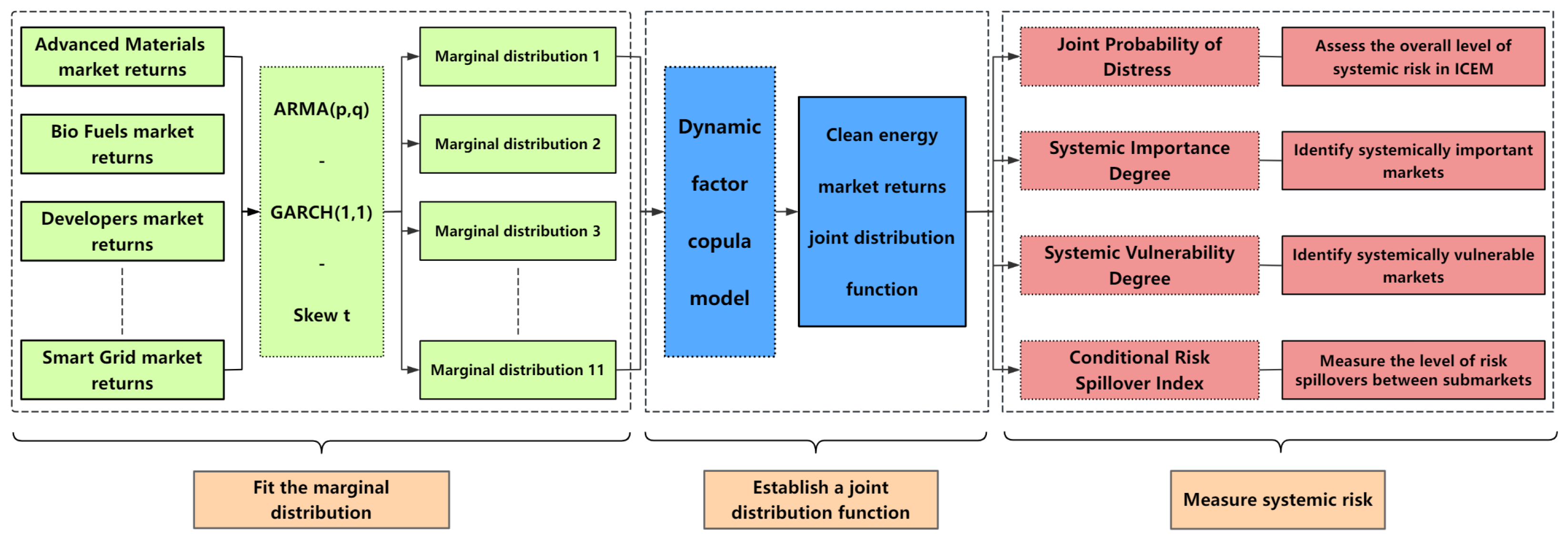
Therefore, this study uses the skewed t distribution dynamic factor copula model to characterize the overall interdependence structure of the international clean energy market and combines the GARCH model to characterize the asymmetry of individual return volatility to conduct systemic risk measurement and regulatory research. The main contribution of the article is as follows. Firstly, the construction of all systemic risk measurement indicators is based on the joint distribution of the entire system, which can better characterize the heavy-tailed, time-varying, asymmetric, and nonlinear dependence structure of financial data in high-dimensional situations, fully considering the correlation between the entire system rather than just the dependence between pairs. Secondly, a unified framework based on joint distribution was established to provide systemic risk measurement indicators for the international clean energy market in different dimensions. The joint probability of distress (JPD) degree was used to measure the probability of collective outbreak risk in the quantum industry market, and the degree of systemic vulnerability and systemic importance were measured. The interdependence of the international clean energy market as a whole and locally was fully considered to identify systemically important markets and systemically vulnerable markets. Thirdly, a conditional risk-spillover index (CRSI) was constructed based on the copula-dependent structure to generate simulated return sequences, which was used to evaluate the level of risk spillover between 11 subindustry markets during periods of concentrated systemic risk outbreaks. Overall, this study comprehensively analyzes and quantifies the systemic risks in the international clean energy market from different perspectives by constructing the ARMA-GARCH-Skew t model and the dynamic factor copula model, providing an important theoretical and empirical basis for formulating more effective macro prudential regulatory policies and helping to enhance the stability and sustainable development capacity of the clean energy market. It should be pointed out that the systemic importance here is stronger than the correlation between subindustry markets.

The remainder of the article is constructed as follows: The second part provides a comprehensive review of the relevant literature. The third part introduces the methodology. The fourth part provides an overview of data sources and basic data analysis. The fifth part presents empirical results on the measurement of systemic risk, systemic importance, systemic vulnerability, and risk-spillover levels. The sixth part summarizes the research conclusions.

2. Literature Review

Systemic risk has always been a focus of academic attention. Benoit et al. (2013) [11] defined systemic risk as the risk that causes a large number of market participants to suffer severe losses simultaneously and rapidly spread throughout the entire system, characterized by common changes (correlations) between most or all parts of the system. Acharya et al. (2017) [12] further described systemic risk, emphasizing that this risk is not limited to the failure of individual institutions but involves a chain reaction of the entire financial system. Adrian and Brunnermeier (2011) [13] pointed out that systemic risk reflects the vulnerability of financial institutions to external shocks, which is reflected through the high correlation between financial institutions. Kaufman and Scott (2003) [14] argue that systemic risk not only comes from the interdependence between financial institutions but also includes regulatory and policy uncertainty, which may exacerbate panic and overreaction among market participants. Overall, systemic risk is a multidimensional concept that encompasses interdependence among market participants, common changes in financial assets, and the impact of external shocks on system stability.

Systemic risk measurement plays an important role in financial risk management. Early risk measurement methods, such as Value at Risk (VaR) [15] and Expected Shortfall (ES) [16], mainly focus on individual risks of individual financial institutions and do not fully consider the interdependence and feedback effects between institutions and the financial system. In recent years, research has gradually shifted towards more comprehensive methods, including tail dependence analysis and $“$portfolio based” measurement [17]. The tail dependence analysis method measures systemic risk by examining the profit and loss dependence relationship between institutions and systems under extreme shocks. Representative research methods include Conditional Value at Risk (CoVaR), $\Delta$CoVaR, Conditional Expected Shortfall (CoES), $\Delta$CoES, etc. [18,19]. For example, Zhang et al. (2023) [20] used the copula–DCC–GARCH model and explored the systemic risk spillover between multiple financial sectors and the stock market in China by calculating CoVaR and $\Delta$CoVaR. They found that there is a highly dynamic correlation between the financial sector and the stock market, and the banking industry is an important source of systemic risk in China. Gu et al. (2022) [21] combined extreme value theory (EVT) and dynamic mixed Copula (DM Copula) function to estimate CoES and applied it to China’s financial market. They found that EVT can more accurately fit the tail distribution of the index, while the new dynamic mixed Copula function better captures the complex correlations between the financial sector and the system. Unlike tail dependence analysis, the $“$portfolio based” measurement method measures systemic risk by evaluating the contribution of a single financial institution (or asset) to the overall financial system (or asset portfolio) risk. Representative methods include Component Expected Shortfall (CES), Marginal Expected Shortfall (MES), Systemic Expected Shortfall (SES), SRISK, etc. [12,22,23]. For example, Manguzvane and Ngobese (2023) [24] used CES to quantify the contribution of important banks and insurance companies in the South African system to the overall systemic risk and found that the ranking results obtained by the CES method were highly consistent with the D-SIB capital surcharge set by regulatory authorities, verifying the accuracy of CES in risk measurement. Armanious (2024) [25] used MES and SRISK to evaluate the systemic risk of the Euro financial system and found that SRISK tends to assign higher systemic risk scores to large institutions, while MES is more easily attracted to interrelated institutions.

With the continuous development and volatility of the energy market, various extreme events have occurred frequently, making the accurate measurement and management of systemic risks particularly important. Correspondingly, the above measurement methods have also been widely applied in the systemic risk analysis of energy markets. Marimoutou et al. (2009) [26] applied extreme value theory to the oil market and found that conditional extreme value theory has significant improvements in predicting VaR compared to traditional methods. Chen and Lv (2015) [27] found, based on EVT, that there is a positive extreme dependence relationship between the Chinese stock market and global crude oil prices, which will further strengthen during economic crises. Ahmed et al. (2022) [28] used EVT to study the tail risk, systemic risk, and spillover effect between crude oil and precious metals and found that except for the COVID-19 pandemic, crude oil and precious metals showed relatively low tail risk during the crisis period. Ren et al. (2023) [29] studied the extreme risk-spillover effects between the international crude oil market and the Chinese energy futures market by constructing a GARCH-EVT-VaR model and found the dependence and vulnerability of the Chinese energy sector to the international oil market. Liu et al. (2021) [30] used a binary copula model and CoVaR system risk indicators to study the time-varying dependence and risk-spillover effects between the GB market and the CE market and found a positive and asymmetric risk-spillover relationship between the GB and CE stock markets. By using CoVaR and Conditional Expectation Value at Risk (CoEVaR), Syuhada et al. (2024) [31] investigated the interconnectivity and systemic risk between clean energy markets and fossil-fuel-based $“$dirty” energy markets. They found that crude oil, heating oil, and industry clean energy indices were highly interconnected, but this connectivity weakened after the 2015 Paris Climate Agreement. Tiwari et al. (2020) [32] used the CoVaR and MES methods to analyze the dependence and risk spillover between the crude oil market and the stock markets of G7 countries and found that the fluctuation of oil prices has a particularly significant impact on the returns of G7 stock markets, especially the Canadian stock market, during market turbulence. Zhao et al. (2023) [33] constructed a GARCH-EVT-Copula-CoVaR model framework based on the GARCH model, Copula function, and CoVaR method and found that international oil prices have positive risk-spillover effects on different industries in China. Tian et al. (2022) [34] used the Generalized Autoregressive Conditional Heteroskedasticity Conditional Quantile Regression (GARCH-CQR) model to estimate the spillover effects of downside risk (DCoVaR) and upside risk (UCoVaR) of the oil market on the stock market at different risk levels and found that downside risk spillover was greater than upside risk spillover. Janda et al. (2022) [35] used three multivariate GARCH models (CCC, DCC, and ADCC) to study the dynamic correlation, return, and volatility spillover effects between clean-energy-related stocks in China and the United States, oil prices, and technology company stocks. They found that compared with technology stocks, the correlation between clean energy company stock prices and oil prices was stronger. The above research mainly focuses on the interdependence between two markets but has not fully addressed the systemic risk problem involving multiple markets.

With the continuous development of complex network theory and the increasing interdependence of various components within the energy market, some researchers have begun to use network-based risk measurement methods to analyze systemic risks in the energy market. Deng et al. (2023) [36] explored the dynamic risk-spillover effects between China’s clean energy market and non-ferrous metal market during the COVID-19 pandemic through complex network analysis and found that the pandemic significantly increased the volatility spillover between markets and changed the risk transmission path. Mensi et al. (2024) [37] used quantile vector autoregression (QVAR) to investigate the dynamic spillover effects between green bonds, renewable energy, and the sustainability markets of G7 countries at different quantiles and constructed a network model to quantify and visualize the degree of interdependence and dependence between markets. Gong et al. (2023) [38] used the QVAR model and network analysis method to study the tail risk-spillover effects of the international energy market under different states and frequency domains. They found that the extreme risk-spillover effects of the clean energy market were more significant, and long-term risk spillover dominated the overall market. Zhao et al. (2024) [39] used the tail risk-spillover network (TRSN) and tail event driven network (TENET) methods to simulate the dynamic tail risk-spillover process of the international energy market in the context of major events and found that the renewable energy market had a greater systemic risk contribution during the Paris Agreement and COVID-19, while the impact of the fossil energy market during the Russia–Ukraine conflict was more significant. Foglia et al. (2024) [40] used a tail event-driven network model to study the correlation between tail risk spillovers of clean energy and oil companies from 2011 to 2021.

From the above research, it can be seen that the core of systemic risk measurement in the energy market lies in evaluating the interdependence between institutions and measuring the spillover effects between different institutions. In the energy market, price fluctuations and policy changes often bring significant nonlinear risk contagion effects, requiring more flexible and accurate measurement tools. In this context, the Copula function has become an important tool for researchers due to its unique advantages. The Copula function can construct a joint distribution function that separates the marginal distribution of individual institutions from the joint dependency structure of the system. This not only allows for the individual modeling of heterogeneity among institutions but also captures changes in interdependence when systemic risks occur, providing more accurate risk measurement. Tiwari et al. (2021) [41] used a Dependence-Switching Copula (DSC) to explore the dependency structure between oil prices and stock returns of clean energy and technology companies under different market conditions. They found asymmetric dependence between oil prices and clean energy stocks and symmetric dependence between oil prices and technology stocks. Naeem et al. (2021) [42] found that green bonds exhibit negative extreme tail dependence with crude oil, heating oil, gasoline, and coal while exhibiting positive extreme tail dependence with natural gas, based on the time-varying optimal copula (TVOC) model analysis.

With the continuous increase in data dimensions, traditional statistical methods often struggle to handle the complex dependency structures in high-dimensional financial data. Oh and Patton (2018) [43] proposed a dynamic factor Copula model that incorporates the Generalized Autoregressive Score (GAS) model proposed by Creal (2013) [44] into the factor Copula model. Wang and Liang (2020) [45] used the dynamic factor Copula model to measure the systemic risk of Chinese banks and identify system importance and vulnerability. Ouyang et al. (2022) [46] used the dynamic factor Copula model to measure systemic risk in the Chinese commodity market and explored the relationship between systemic risk and macroeconomics. Chen et al. (2023) [47] studied the dynamic dependency relationships between Chinese real industries based on a dynamic factor copula model and found that the model had the highest accuracy in estimating the minimum ES. The dynamic factor Copula model not only effectively captures dynamic dependency relationships in high-dimensional data but also provides new ideas and methods for measuring systemic risks.

There are still several shortcomings in the research on systemic risk measurement in the energy market. Firstly, current research on the clean energy market mainly focuses on selecting comprehensive stock indices or individual stock indices (such as renewable energy such as solar and wind energy), but there is a lack of research on other subindustry markets within the clean energy system, which fails to deeply characterize the interrelationships between each subindustry market. Secondly, classic systemic risk indicators such as CoVaR, $\Delta$CoVaR, and MES mainly focus on the pairwise interdependence between markets but do not fully consider the overall systemic risk of multiple markets. Finally, although tail-risk-based network models can reveal the dependency relationships between different markets in the system, these models often focus on the bilateral or multilateral dependency structures of local markets, which may have shortcomings in the global characterization of systemic risk and fail to fully capture the complex interaction effects between all markets.

Therefore, this article will study the various subindustry markets that make up the international clean energy market as independent markets. It will capture the yield characteristics of various subindustry markets through GARCH models and use a dynamic factor copula model to measure the systemic risk of the international clean energy market. In addition, it will identify the systemic vulnerability and importance of various subindustry markets and analyze the level of risk spillover between markets to provide a more comprehensive risk assessment.

3. Methodology

This study mainly divides the measurement of systemic risk into three steps: the first step is to use the ARMA-GARCH-Skew t model to model the returns of the subindustry market and obtain the marginal distribution function. The second step is to apply a dynamic factor copula model to the marginal distribution function to obtain a joint distribution function, which describes the correlation of the international clean energy market. The third step is to calculate the joint probability of distress of the entire system through a joint distribution function to measure the overall level and dynamic evolution of systemic risk. The indicators of systemic vulnerability and systemic importance are introduced to identify the systemic vulnerability and systemic importance of a single subindustry market, and a conditional risk-spillover index is constructed to measure the level of risk spillover between subindustry markets. The specific process is shown in Figure 1.

3.1. Factor Copulas

Factor modeling is widely used in high-dimensional time series analysis to effectively solve the $“$curse of dimensionality” problem. Oh and Patton (2017) [48] proposed a new factor copula model based on a latent factor structure. This paper uses a single-factor copula model to describe the dependence structure of latent vector random variable $X_t\equiv {(X_{1,t},\dots ,X_{N,t})}^{\prime }$, with the following model structure:

$$X_{i,t}={\lambda }_{i,t}\left({\gamma }_{\lambda }\right)Z_t+{\epsilon }_{i,t},i=1,2,\dots ,N$$

$$\mathrm{where}{Z}_t\sim F_{Z,t}\left({\gamma }_Z\right),{\epsilon }_{i,t}\sim \mathrm{iid}{F}_{\epsilon ,t}\left({\gamma }_{ϵ}\right),$$

$$Z_t\perp \perp {\epsilon }_i\forall i.$$

Here, $F_{z,t}\left({\gamma }_z\right)$ and $F_{\epsilon ,t}\left({\gamma }_{\epsilon }\right)$ represent the parameterized univariate distributions of the common factor and idiosyncratic factors, respectively. The common factor $Z_t$ captures common changes and market trends across the system, while the idiosyncratic factor ${\epsilon }_{i,t}$ describes each variable’s unique impact given the common factor. ${\lambda }_{i,t}\left({\gamma }_{\lambda }\right)$ represents the time-varying weight ${\lambda }_{i,t}$, whose time variation is regulated by the parameter ${\gamma }_{\lambda }$. Let the marginal distribution of $X_{i,t}$ be denoted as $G_{i,t}$. According to the conditional Sklar’s theorem, the joint distribution of $X_t$ can be composed of its conditional marginal distribution functions and conditional copula function:

$$X_t\sim G_t=C_t(G_{1,t}\left(\gamma \right),\dots ,G_{N,t}\left(\gamma \right);\gamma )$$

$$\mathrm{where}\gamma \equiv {[{\gamma }_z^{\prime },{\gamma }_{\epsilon }^{\prime },{\gamma }_{\lambda }^{\prime }]}^{\prime }.$$

To reduce estimation complexity, this paper simplifies the model. Specifically, we set fixed shape parameters for the common and idiosyncratic factors ($Z_t$ and ${\epsilon }_{i,t}$). The common factor $Z_t$ follows a skewed t distribution proposed by Hansen (1994) [49] with degrees of freedom parameter ${\nu }_Z$ and skewness parameter ${\psi }_Z$, while the idiosyncratic factor ${\epsilon }_{i,t}$ follows a t distribution with degrees of freedom parameter ${\nu }_{\epsilon }$. The skewed t distribution, with its ability to capture skewness and fat tails, can better capture asymmetry and extreme risk events in financial markets.

Since the copula of X does not have an explicit solution for most factor combinations (such as the skewed t distribution and t distribution used in this paper), numerical integration methods are employed to solve this problem. Specifically, the Gaussian–Legendre quadrature formula is used to integrate over the common factor for maximum likelihood estimation.

3.2. GAS Model

In order to capture the dynamic characteristics of the dependency structure, the GAS model from Creal et al. (2013) [44] is used. The GAS model has strong inclusiveness, able to encompass a variety of existing successful models, and effectively improves model fitting through optimization algorithms. In this paper, the GAS model is combined with the factor copula model to estimate the dynamic changes in factor loadings ${\lambda }_{i,t}$:

$$\mathrm{let}{U}_t|F_{t-1}\sim C\left({\delta }_t\left(\gamma \right)\right)$$

$$\mathrm{then}{\delta }_t=\omega +B{\delta }_{t-1}+A{s}_{t-1}$$

$$\mathrm{where}{s}_{t-1}=S_{t-1}{\nabla }_{t-1}$$

$${\nabla }_t={\displaystyle \frac{\partial logc(u_{1,t},\dots ,u_{N,t};{\delta }_{t-1})}{\partial {\delta }_{t-1}}}$$

Here, $S_t$ represents the scaling matrix (inverse Hessian or its square root).

Referring to the simplification method from Oh and Patton (2018) [43], it is assumed that the coefficient matrices B and A are diagonal matrices, and the elements on their diagonals are represented by scalar parameters $\beta$ and $\alpha$, respectively. Meanwhile, the matrix $S_t$ is set to the identity matrix I. The parameters of the copula model are logarithmically transformed, so the logarithm of the factor loadings in the GAS model can be expressed as

$$log{\lambda }_{i,t}={\omega }_i+\beta log{\lambda }_{i,t-1}+\alpha s_{i,t-1}$$

$$s_{i,t}={\displaystyle \frac{\partial logc(u_t;{\lambda }_t,{\nu }_z,{\psi }_z,{\nu }_{\epsilon })}{\partial log{\lambda }_{i,t}}},i=1,2,\dots ,N.$$

3.3. Joint Probability of Distress (JPD)

In this paper, we define a risk event in the clean energy market as a situation where the return is below a certain threshold:

$$D_{i,t}\equiv 1\{R_{i,t}<c_i\}$$

where $R_{i,t}$ represents the return of the clean energy market i at time t and $c_i$ is the return quantile (in the empirical part of this paper, the 5% quantile is used). A key characteristic of systemic risk is that a large number of markets or institutions simultaneously suffer from tail risk shocks. The concentration of systemic risk can be measured by the frequency of collective risk events.

Following the study by Oh and Patton (2018) [43], we use the joint probability of distress (JPD) model to measure the probability of tail risk events occurring simultaneously over different periods, thereby assessing the overall level of systemic risk in the international clean energy market. Specifically, JPD is defined as follows:

$$JP{D}_{t,k}\equiv P_t\left[\left({\displaystyle \frac{1}{N}}\sum _{i=1}^N{D}_{i,t+1}\right)\ge {\displaystyle \frac{k}{N}}\right]$$

where $JP{D}_{t,k}$ represents the probability that at least k clean energy markets will experience risk events at time $t+1$, given the information known prior to time t.

3.4. Systemic Vulnerability and Importance Measurement

Drawing on the research of Wang and Liang (2020) [45], two indicators, SVD (Systemic Vulnerability Degree) and SID (Systemic Importance Degree), are introduced to evaluate the systemic vulnerability and importance of various clean energy markets.

3.4.1. Systemic Vulnerability Degree (SVD)

The degree of systemic vulnerability is used to measure the degree to which a market is impacted during the risk contagion process. This indicator calculates the probability that market i is in a risk state at time $t+1$, under the condition that at least k market risk events occur at time $t+1$, that is, the Conditional Probability of Distress (CoPD). The formula is as follows:

$$CoP{D}_{i,t,k}\equiv E_t[D_{i,t+1}\mid M_{i,t+1}\ge k]$$

where $M_{i,t+1}={\sum }_{j=1,j\ne i}^N{D}_{j,t+1}$ indicate the number of markets in the system at time $t+1$ when risk events occur, except for the $i-th$ market.

In this study, $k=N/2$ is set and the Systemic Vulnerability Degree (SVD) is defined as

$$SV{D}_{i,t}\equiv CoP{D}_{i,t,N/2}.$$

In tail risk monitoring, it is necessary to measure both global and local risks uniformly. The market with more than half of the condition $M_{i,t+1}$ values in the SVD indicator covers both local market crisis events (i.e., some markets are in a risk state) and global crisis events (i.e., all markets are in a risk state when $k=N-1$). This indicator fully considers the vulnerability of individual markets under global and local crisis events and characterizes the correlation structure of the entire international clean energy market system under different situations.

3.4.2. Systemic Importance Degree (SID)

The degree of systemic importance is used to measure the risk contribution of a market to the overall system, i.e., its risk-spillover effect. This index calculates the probability of a collective risk event occurring in the system under the condition that a risk event occurs in market i at time $t+1$, namely the Conditional Contribution of Distress (CoCD). The formula is as follows:

$$CoC{D}_{i,t,k}\equiv E_t[M_{i,t+1}\ge k\mid D_{i,t+1}]$$

and similarly, set $k=N/2$ and define the Systemic Importance Degree (SID) as

$$SI{D}_{i,t}\equiv CoC{D}_{i,t,N/2}.$$

3.5. Measurement of Risk-Spillover Level

The Conditional Risk-Spillover Index (CRSI) is used to measure the level of risk spillover between submarkets, controlling for the condition that no other markets experience risk events. The index calculates the probability that market j experiences a risk event at time $t+1$, given that market i experiences a risk event while no other markets do. The formula is as follows:

$$CRS{I}_{i,j}\equiv E_t\left[D_{j,t+1}\mid D_{i,t+1}=1\mathrm{and}\sum _{k\ne i,j}{D}_{k,t+1}=0\right]$$

$$-E_t\left[D_{j,t+1}\mid D_{i,t+1}=0\mathrm{and}\sum _{k\ne i,j}{D}_{k,t+1}=0\right]$$

where ${\sum }_{k\ne i,j}{D}_{k,t+1}$ represents the number of markets experiencing risk events at time $t+1$, excluding markets i and j.

4. Data Description

4.1. Data Source

With the development of the global economy and society, financial market indices are not only a reflection of company performance but also a barometer of economic conditions and investor confidence. The volatility of financial market indices related to clean energy can profoundly reflect the dynamic changes in the clean energy market. To comprehensively analyze the systemic risk of the international clean energy market, the NASDAQ OMX Clean Energy Index series is selected as the research object. This index series provides a more comprehensive set of indices for tracking the global environment and clean energy industry and its subsectors [50]. Specifically, the NASDAQ OMX Clean Energy Index can be divided into four categories, as shown in

Table 1. NASDAQ OMX Clean Energy Index.

Category	Index	Symbol	Description
Advanced materials	NASDAQ OMX Advanced Material Index	M1	Tracks companies producing materials that support renewable technologies or reduce reliance on petroleum-based products
Bio/Clean fuels	NASDAQ OMX Bio/Clean Fuels Index	M2	Tracks producers of plant-based fuels used as alternatives to petroleum-based transportation fuels
Renewable energy	NASDAQ OMX Developer/Operator Index	M3	Tracks developers and operators of solar, wind, and other renewable energy projects
	NASDAQ OMX Fuel Cell Index	M4	Tracks energy producers using fuel cell technology
	NASDAQ OMX Geothermal Index	M5	Tracks companies specializing in geothermal energy production
	NASDAQ OMX Solar Index	M6	Tracks solar power production companies
	NASDAQ OMX Wind Index	M7	Tracks companies involved in wind energy production
Energy efficiency	NASDAQ OMX Energy Management Index	M8	Tracks companies offering solutions for reducing energy use through advanced management systems like efficient motors and process controls
	NASDAQ OMX Energy Storage Index	M9	Tracks companies advancing energy storage technologies like batteries
	NASDAQ OMX Green IT Index	M10	Tracks IT solutions providers focusing on energy efficiency through technologies like data center optimization and virtualization
	NASDAQ OMX Smart Grid Index	M11	Tracks companies enhancing grid reliability and intelligence through modernization solutions

Source: NASDAQ and Pham (2019) [50].

. Treating each market index as an independent market for analysis, there are a total of 11 markets.

Considering that the NASDAQ OMX Clean Energy Index has been trading since 18 October 2010, this study selects the period from 18 October 2010, to 17 May 2024, for research, with a total of 3419 observations, all of which are from investment websites.

4.2. Basic Data Analysis

Table 2. Descriptive statistics of logarithmic returns for 11 clean energy indices.

Market	Mean	Min	Max	Std.	Skewness	Kurtosis
M1	−0.0012	−6.5879	7.2790	0.5274	1.2832	96.6234
M2	−0.0007	−7.1408	5.8709	0.7669	−0.4187	32.8268
M3	−0.0011	−8.0107	6.6280	0.4179	−2.8744	197.2819
M4	−0.0004	−8.0017	6.9180	0.5167	−0.9020	103.1280
M5	0.0004	−7.9316	7.9212	0.6993	−0.1934	52.9274
M6	−0.0013	−5.8403	5.9674	0.4002	0.6544	149.9079
M7	−0.0011	−8.0668	6.4508	0.4135	−3.0220	176.1471
M8	−0.0011	−7.3122	8.0054	0.5812	1.1994	90.1047
M9	−0.0007	−6.3651	7.9862	0.5279	1.4577	97.2519
M10	−0.0010	−8.0199	8.0117	0.5326	−0.9043	123.7959
M11	−0.0011	−7.9540	7.9649	0.4566	0.5270	140.0699

presents the basic statistics of logarithmic returns for 11 clean energy indices. Skewness analysis shows that the logarithmic return sequences of all clean energy markets follow an asymmetric distribution, and the kurtosis coefficients are all greater than 3, indicating a sharp and thick-tailed distribution of market returns.

5. Empirical Results and Analysis

5.1. Fit Marginal Distribution

First, the marginal distribution of the return series for each clean energy market is fitted. According to the ADF test, all series are stationary at the $1\%$ significance level. Based on the J-B test, the return distributions of each market are significantly different from the normal distribution. The LB test and the ARCH-LM test with 20 lags indicate that all series exhibit significant autocorrelation and ARCH effects. To better capture the characteristics of fat tails and asymmetry in the data, the ARMA(p,q)-GARCH(1,1)-Skew t model is used to fit the marginal distribution. The model is formulated as follows:

$$\begin{array}{c}\hfill \left\{\begin{array}{cc}{R}_{i,t}\hfill & ={\phi }_{i,0}+\sum _{n=1}^p{\phi }_{i,n}{R}_{i,t-n}+{\epsilon }_{i,t}-\sum _{m=1}^q{\theta }_{i,m}{\epsilon }_{i,t-m}\hfill \\ {\epsilon }_{i,t}\hfill & ={\sigma }_{i,t}{\eta }_{i,t},{\eta }_{i,t}\sim \mathrm{iid}Skewt({\nu }_i,{\psi }_i)\hfill \\ {\sigma }_{i,t}^2\hfill & ={\omega }_i+{\alpha }_i{\epsilon }_{i,t-1}^2+{\beta }_i{\sigma }_{i,t-1}^2\hfill \end{array}\right.\end{array}$$

where ${\phi }_{i,0}$ is the constant term of the ARMA(p,q) model, ${\phi }_{i,n}$ is the autoregressive coefficient, ${\epsilon }_{i,t}$ is the residual term, following Hansen’s (1994) [49] skewed t distribution, where ${\nu }_i$ and ${\psi }_i$ determine the degrees of freedom and skewness of the skewed t distribution, respectively; ${\theta }_{i,m}$ is the moving average coefficient; ${\alpha }_i$ is the ARCH parameter; and ${\beta }_i$ is the GARCH parameter.

Table 3. Marginal distribution parameter estimation results.

Market	M1	M2	M3	M4	M5	M6
${\phi }_{i,0}$	−0.0002 (−0.7124)	0.0004 (0.5717)	−0.0006 *** (−2.935)	0.0013 *** (2.7605)	0.0001 (0.1604)	−0.0006 * (−1.9556)
${\phi }_{i,1}$	0.8450 *** (9.6248)	1.6743 *** (3220.3832)	0.0206 (0.1131)	0.8166 *** (8.2241)	−1.1620 *** (−7146.3373)	0.0196 (1.1041)
${\phi }_{i,2}$	−0.0073 (−0.3221)	−0.9100 *** (−1960.0041)	−0.0809 (−0.5119)	−0.7198 *** (−5.0202)	0.1118 *** (739.0500)	0.0177 (1.1027)
${\phi }_{i,3}$	−0.0055 (−0.3261)	−0.0183 *** (−42.4145)	0.5438 *** (3.8696)	0.5050 *** (4.2985)	0.6102 *** (5991.0197)	0.0028 (0.1895)
${\phi }_{i,4}$				0.0013 (0.0966)		−0.0170 (−1.2772)
${\phi }_{i,5}$				−0.0021 (−0.2575)		−0.0055 (−0.4936)
${\theta }_{i,1}$	−0.8473 *** (−9.7802)	−1.6928 *** (−3111.0619)	0.0092 (0.0505)	−0.8373 *** (−8.5849)	1.1070 *** (8059.7525)
${\theta }_{i,2}$		0.9416 *** (1983.4071)	0.0695 (0.4265)	0.7098 *** (5.0298)	−0.2040 *** (−8726.5037)
${\theta }_{i,3}$			−0.5483 *** (−3.8174)	−0.5223 *** (−4.7530)	−0.6574 *** (−5217.0239)
${\theta }_{i,4}$			−0.0206 (−1.2585)		−0.0003 (−0.6600)
${\theta }_{i,5}$			0.0279 * (1.6845)		−0.0039 *** (−11.3083)
${\omega }_i$	0.0000 *** (4.2388)	0.0010 *** (9.1804)	0.0000 *** (7.7313)	0.0005 *** (7.2122)	0.0004 *** (8.5149)	0.0001 *** (7.9681)
${\alpha }_i$	0.2942 *** (17.3123)	0.6886 *** (14.8922)	0.3590 *** (17.5551)	0.5326 *** (10.6172)	0.6646 *** (16.8748)	0.4612 *** (16.6045)
${\beta }_i$	0.7048 *** (50.2256)	0.3104 *** (14.4611)	0.6400 *** (43.0400)	0.4664 *** (14.2168)	0.3344 *** (15.2606)	0.5378 *** (30.1923)
${\psi }_i$	1.0675 *** (55.5737)	1.0872 *** (58.4626)	1.0623 *** (51.1134)	1.0233 *** (58.4611)	1.1119 *** (59.0161)	1.0263 *** (59.0419)
${\nu }_i$	3.8484 *** (24.8662)	2.7177 *** (44.7174)	4.2049 *** (22.6960)	2.5357 *** (43.6774)	2.8671 *** (42.8089)	3.0789 *** (35.0408)
LogLik	5279.0720	3596.6940	7425.9620	5461.7680	4480.0690	6462.5810
Market	M7	M8	M9	M10	M11
${\phi }_{i,0}$	−0.0003 (−1.5380)	−0.0008 *** (−3.8183)	0.0003 (0.7910)	−0.0011 *** (−3.4733)	−0.0004 * (−1.7453)
${\phi }_{i,1}$	1.7520 *** (95.7582)	0.9371 *** (235.0407)	0.8391 *** (5.2137)	0.7895 *** (16.7253)	1.7484 *** (192.9443)
${\phi }_{i,2}$	−1.2560 *** (−34.1595)	−0.0236 (−1.4782)	−0.0553 ** (−2.3052)	0.0359 ** (2.2971)	−2.2398 *** (−238.0214)
${\phi }_{i,3}$	0.3567 *** (6.5217)	−0.0043 (−0.1928)	0.0181 (0.8445)		1.3892 *** (189.1197)
${\phi }_{i,4}$	−0.0040 (−0.1213)	−0.0120 (−0.5970)	−0.0380 * (−1.9259)		−0.6015 *** (−32.0232)
${\phi }_{i,5}$	0.0102 (0.6637)	0.0362 ** (2.5598)	0.0193 (1.0930)
${\theta }_{i,1}$	−1.7545 *** (−2353.3969)	−0.9433 *** (−267.1463)	−0.7956 *** (−4.9973)	−0.8437 *** (−17.9024)	−1.7082 *** (−1279.5498)
${\theta }_{i,2}$	1.2541 *** (933.7809)				2.1618 *** (12895.7617)
${\theta }_{i,3}$	−0.3620 *** (−10.2314)				−1.3121 *** (−360.8111)
${\theta }_{i,4}$					0.5548 *** (26.6997)
${\theta }_{i,5}$
${\omega }_i$	0.0000 *** (7.9033)	0.0000 *** (5.1613)	0.0001 *** (7.3062)	0.0001 *** (6.7476)	0.0000 *** (4.2559)
${\alpha }_i$	0.3249 *** (16.7573)	0.3971 *** (19.7712)	0.3756 *** (14.7527)	0.5290 *** (16.1023)	0.2674 *** (17.1808)
${\beta }_i$	0.6741 *** (44.4860)	0.6019 *** (39.4101)	0.6234 *** (35.4739)	0.4700 *** (21.1233)	0.7316 *** (56.9000)
${\psi }_i$	1.0348 *** (56.5116)	1.0655 *** (56.1808)	1.0737 *** (53.3635)	1.0487 *** (55.2222)	1.0967 *** (54.6823)
${\nu }_i$	3.7207 *** (26.9597)	3.8532 *** (27.5073)	3.3943 *** (26.5037)	3.1744 *** (32.5203)	4.1127 *** (23.7702)
LogLik	7373.3320	5908.8510	5548.5710	5971.6550	6024.1910

Note: ***, **, and * represent significance at the $1\%$, $5\%$, and $10\%$ levels, respectively, with the value of t shown in parentheses.

presents the parameter estimation results for the marginal distributions. The first autoregressive coefficient and the first moving average coefficient are significant for most markets, indicating that most markets exhibit serial correlation and short-term volatility in returns. In the GARCH model, the ${\alpha }_i$ and ${\beta }_i$ parameters are significant and positive for all 11 markets, suggesting significant volatility clustering effects in the returns. Moreover, the degrees of freedom parameter ${\nu }_i$ is significant for all 11 markets, indicating that return shocks exhibit fat tails. The skewness parameter ${\psi }_i$ is also significant and greater than 1, indicating a right-skewed return distribution.

Table 4. Test results for standardized residual series and copula data.

Market	LB	p-Value	ARCH-LM	p-Value	KS	p-Value
M1	0.0413	0.8390	0.0004	0.9832	0.0003	1.0000
M2	0.5539	0.4567	0.0553	0.8140	0.0003	1.0000
M3	0.0102	0.9196	0.0008	0.9774	0.0003	1.0000
M4	0.0698	0.7917	0.0033	0.9545	0.0003	1.0000
M5	0.0608	0.8052	0.0013	0.9715	0.0003	1.0000
M6	0.1171	0.7319	0.0040	0.9494	0.0003	1.0000
M7	0.2421	0.6227	0.0421	0.8374	0.0003	1.0000
M8	0.0676	0.7949	0.0087	0.9258	0.0003	1.0000
M9	0.0049	0.9443	0.0003	0.9852	0.0003	1.0000
M10	0.0129	0.9097	0.0067	0.9349	0.0003	1.0000
M11	0.0137	0.9067	0.0012	0.9725	0.0003	1.0000

presents the test results for the standardized residual series and copula data. The results of the Ljung–Box test and ARCH test show that all p-values are greater than 0.05, indicating that the standardized residual series obtained after fitting the marginal distribution models no longer exhibit autocorrelation or heteroscedasticity. The results of the KS test suggest that the transformed copula data follow a uniform distribution on $[0,1]$. Therefore, the ARMA(p,q)-GARCH(1,1)-Skew t model constructed in this paper is reasonable, and it is feasible to further establish a dynamic factor copula model.

5.2. Establish a Dynamic Factor Copula Function

Table 5. Parameter estimation results of the dynamic factor copula model.

Parameter	$\mathit{\alpha }$	$\mathit{\beta }$	${\mathit{\nu }}_{\mathit{z}}$	${\mathit{\psi }}_{\mathit{z}}$	${\mathit{\nu }}_{\mathit{\epsilon }}$
Estimate	0.0726	0.9909	61.1747	0.1163	4.616

presents the parameter estimation results of the dynamic factor copula model, where the value of $\beta$ is 0.9909, which is close to 1, indicating that the estimated load factor has high persistence. ${\nu }_z$ and ${\nu }_{ϵ}$ reflect the fat-tail characteristics of the common factor and idiosyncratic factors, respectively. The results show that ${\nu }_z$ is greater than ${\nu }_{ϵ}$, suggesting that the idiosyncratic factors of the market are more likely to trigger extreme fluctuations in the international clean energy system than the common factor. ${\psi }_z$ represents the skewness characteristic of the international clean energy market, with a value of 0.1163, which is greater than 0. This is consistent with the estimation results of the marginal distribution model, showing a right-skewed characteristic.

Figure 2 shows the temporal variation of the load factor, which is derived from a simple average of all clean energy markets. It can be seen that the load factor fluctuates with time, ranging from 0.38 to 1.24, and exhibits a clustering effect. According to Naeem et al. (2020) [51], major economic events or extreme situations enhance connectivity between financial markets, while investor confidence weakens when it increases. Since 2011, the correlation of the international clean energy market has rapidly increased, and the European debt crisis has driven an increase of about $70\%$ in the load factor. After 2013, the correlation began to decline, indicating that systemic risks continued to accumulate during the European debt crisis. In mid-2014, the sharp drop in international oil prices led to a further increase in market correlation, but the growth rate was only about $15\%$. The conclusion of the Paris Agreement at the end of 2015 led to a rapid increase in market interdependence, growing by about $40\%$. Subsequently, the withdrawal of the United States from the Paris Agreement, as well as the Sino US trade war in 2018, the COVID-19 outbreak in 2020, the Russia–Ukraine conflict in 2022, and other events, led to increased market connectivity. It can be preliminarily concluded that there is a strong synchronicity between the connectivity of the international clean energy market and systemic risk events.

5.3. Joint Probability of Distress

This study uses Monte Carlo simulation to obtain the joint probability of distress of 11 clean energy markets. In order to improve the accuracy of the simulation, an estimated value is calculated every five trading days with 5000 simulations. Taking $k=6$ as an example to illustrate the selection of the number of defaults k, the result is shown in Figure 3.

From the graph, it can be seen that the systemic risks in the international clean energy market exhibit rapid and multiple outbreaks, and the probability of joint default risk in the entire system can exceed 0.6. The outbreak of systemic risks is closely related to a series of major international events, demonstrating a strong correlation.

Specifically, during the 2011 European debt crisis, the European economy declined, and unemployment rates soared, affecting other global markets. The clean energy industry is facing increasing systemic risks due to tight liquidity, decreased investor risk appetite, and intensified market volatility. In 2014, the Ukrainian crisis led to increased uncertainty in Europe’s natural gas supply, and geopolitical instability further amplified market risks. At the same time, the sharp drop in international oil prices in the second half of the year, coupled with a series of subsequent geopolitical events, intensified the turbulence in the clean energy market, and the risk of joint default significantly fluctuated.

The achievement and implementation of the Paris Agreement is a significant positive for the clean energy market, but it has caused market volatility in the short term. In the fourth quarter of 2017, the passage of the US tax reform bill reduced the tax burden on the clean energy sector and promoted investment in the clean energy industry. In 2018, the US–China trade war led to increased tariffs and supply chain disruptions, exacerbating market uncertainty. At the beginning of 2020, the large-scale outbreak of COVID-19 led to the global blockade and stagnation of economic activities. Energy demand declined significantly, and all energy markets, including clean energy, were severely impacted. After the epidemic, the international clean energy market was relatively stable until the outbreak of the Russia–Ukraine conflict in February 2022. Conflicts have led to drastic fluctuations in global energy prices, supply chain disruptions, and an increased probability of joint defaults in the clean energy market.

Therefore, external events such as economic shocks, geopolitical risks, and changes in environmental policies can all trigger systemic risks in the international clean energy market. Risk contagion is one of the important sources of systemic risk, and this contagion effect is closely related to the connectivity between markets [52]. External shock events typically enhance market connectivity, allowing risk events in one market to spread faster to other markets, ultimately leading to systemic risk outbreaks within the entire international clean energy market. In addition, external shock events can also affect internal information contagion in the market, such as herd behavior and intensified convergence effects, further deepening the severity of systemic risks.

5.4. Systemic Vulnerability

Table 6. Mean SVD across periods.

Market	2010–2013	2014–2015	2016–2017	2018–2019	2020–2021	2022–2024	Overall Mean
M1	0.0725(6)	0.7363(2)	0.5150(2)	0.2798(1)	0.0381(4)	0.1822(2)	0.2805(2)
M2	0.0338(11)	0.1392(11)	0.0000(11)	0.0000(11)	0.0000(11)	0.0000(11)	0.0285(11)
M3	0.0642(8)	0.7285(4)	0.5006(4)	0.2372(5)	0.0351(7)	0.1804(3)	0.2682(4)
M4	0.0560(9)	0.3055(9)	0.0551(9)	0.0096(9)	0.0058(9)	0.0051(9)	0.0696(9)
M5	0.0515(10)	0.2122(10)	0.0202(10)	0.0015(10)	0.0003(10)	0.0017(10)	0.0470(10)
M6	0.0748(5)	0.7478(1)	0.4983(5)	0.2166(6)	0.0379(5)	0.1200(7)	0.2601(6)
M7	0.0795(1)	0.7360(3)	0.5406(1)	0.2696(2)	0.0368(6)	0.1784(4)	0.2835(1)
M8	0.0788(3)	0.6924(7)	0.3980(7)	0.2151(7)	0.0406(1)	0.1250(6)	0.2391(7)
M9	0.0692(7)	0.5596(8)	0.2021(8)	0.0503(8)	0.0286(8)	0.0175(8)	0.1435(8)
M10	0.0762(4)	0.7023(5)	0.5093(3)	0.2566(3)	0.0397(2)	0.1680(5)	0.2698(3)
M11	0.0789(2)	0.7018(6)	0.4551(6)	0.2462(4)	0.0381(3)	0.1833(1)	0.2633(5)

shows the degree of systemic vulnerability of 11 subindustry markets in the international clean energy market over different time periods. The values in parentheses indicate the descending ranking of the SVD mean values for each subindustry market, while the annual mean values reflect the SVD mean values during the study period.

From the table, it can be seen that the SVD of each subindustry market shows similar trends in different time periods, especially during the period of 2014–2015, when the SVD reached its peak and the vulnerability significantly increased. Subsequently, it gradually declined and rose again during the period of 2022–2024. In 2014–2015, the Ukrainian crisis and the sharp drop in international oil prices triggered severe fluctuations in the global energy market, leading to a significant increase in the sensitivity of various subindustry markets to risk events and further exacerbating their vulnerability. Similarly, in 2022, the Russia–Ukraine conflict triggered the instability of the global energy market again, leading to the rise of SVD in various subindustry markets again. This indicates that various subindustry markets are prone to difficulties and exhibit higher systemic fragility when facing major geopolitical risk events.

From the ranking of systemic vulnerability in different subindustry markets at different time periods, the biofuel market (M2), fuel cell market (M4), geothermal market (M5), and energy storage market (M9) have relatively stable systemic vulnerability rankings in various time periods and have always been in a low position. In particular, the rankings of the biofuel market and geothermal market are 11 and 10, respectively. The reason for this is that biofuel technology is mainly used in specific fields such as transportation, and its substitutability is not as wide as solar energy, wind energy, etc., with a limited market size. Geothermal energy, on the other hand, is mainly used in specific regions due to uneven resource distribution, with a smaller global market size and lower volatility. The wind energy market (M7) and advanced material market (M1) have shown high systemic vulnerability in multiple periods, which may be due to the large scale of the wind energy market worldwide, high investment costs, strong dependence on technological progress and policy support, and the widespread application of advanced materials with high research and development and production costs, making them vulnerable to systemic risks.

5.5. Systemic Importance

Table 7. Mean SID across periods.

Market	2010–2013	2014–2015	2016–2017	2018–2019	2020–2021	2022–2024	Overall Mean
M1	0.0522(6)	0.3409(5)	0.0953(5)	0.0276(5)	0.0101(5)	0.0165(5)	0.0851(5)
M2	0.0446(10)	0.1798(11)	0.0000(11)	0.0000(11)	0.0000(11)	0.0000(11)	0.0370(11)
M3	0.0443(11)	0.3057(8)	0.0772(9)	0.0215(8)	0.0078(9)	0.0128(8)	0.0735(9)
M4	0.0486(9)	0.3156(7)	0.0778(7)	0.0128(9)	0.0094(7)	0.0069(9)	0.0740(8)
M5	0.0503(8)	0.2669(10)	0.0340(10)	0.0031(10)	0.0040(10)	0.0039(10)	0.0580(10)
M6	0.0529(5)	0.3454(4)	0.0989(4)	0.0311(5)	0.0103(4)	0.0198(2)	0.0876(4)
M7	0.0515(7)	0.3006(9)	0.0777(8)	0.0215(7)	0.0080(8)	0.0129(7)	0.0746(7)
M8	0.0583(1)	0.3723(2)	0.1241(1)	0.0381(1)	0.0115(2)	0.0278(1)	0.0992(1)
M9	0.0570(3)	0.3881(1)	0.1189(2)	0.0336(2)	0.0143(1)	0.0178(4)	0.0985(2)
M10	0.0533(4)	0.3270(6)	0.0936(6)	0.0272(6)	0.0100(6)	0.0165(6)	0.0830(6)
M11	0.0576(2)	0.3567(3)	0.1062(3)	0.0324(3)	0.0112(3)	0.0190(3)	0.0916(3)

shows the systemic importance levels of 11 subindustry markets in the international clean energy market over different time periods. The values in parentheses indicate the descending ranking of the SID mean values for each subindustry market, while the historical mean values reflect the SID mean values during the study period. From the table, it can be seen that the SID of the 11 subindustry markets shows a similar trend to the degree of systemic vulnerability (SVD) in different periods. Specifically, during the periods of 2014–2015 and 2022–2024, the SID of 11 subindustry markets significantly increased, indicating the amplification effect of major geopolitical events (such as the Ukraine crisis and the sharp drop in international oil prices) on systemic risks. During 2020–2021, SID dropped to the lowest level, which may be due to the global spread of the COVID-19 epidemic, which triggered panic in the market and made investors more sensitive to the risk spillover of clean energy stock prices.

From the ranking of the systemic importance of various subindustry markets at different time periods, the energy management market (M8), energy storage market (M9), smart grid market (M11), and solar energy market (M6) have consistently ranked among the top four in terms of their systemic importance. In particular, the energy management market and energy storage market are ranked 1 and 2, respectively. The reason for this is that energy management systems involve the production, distribution, consumption, and efficiency optimization of energy, and energy storage technology plays a key role in balancing the gap between renewable energy supply and demand. This conclusion is consistent with the research findings of Zhao et al. (2024) [7], indicating that the systemic importance of the energy management market and energy storage market continues to be significant, with strong correlations with other markets, and has a $“$ripple effect” on the entire international clean energy system.

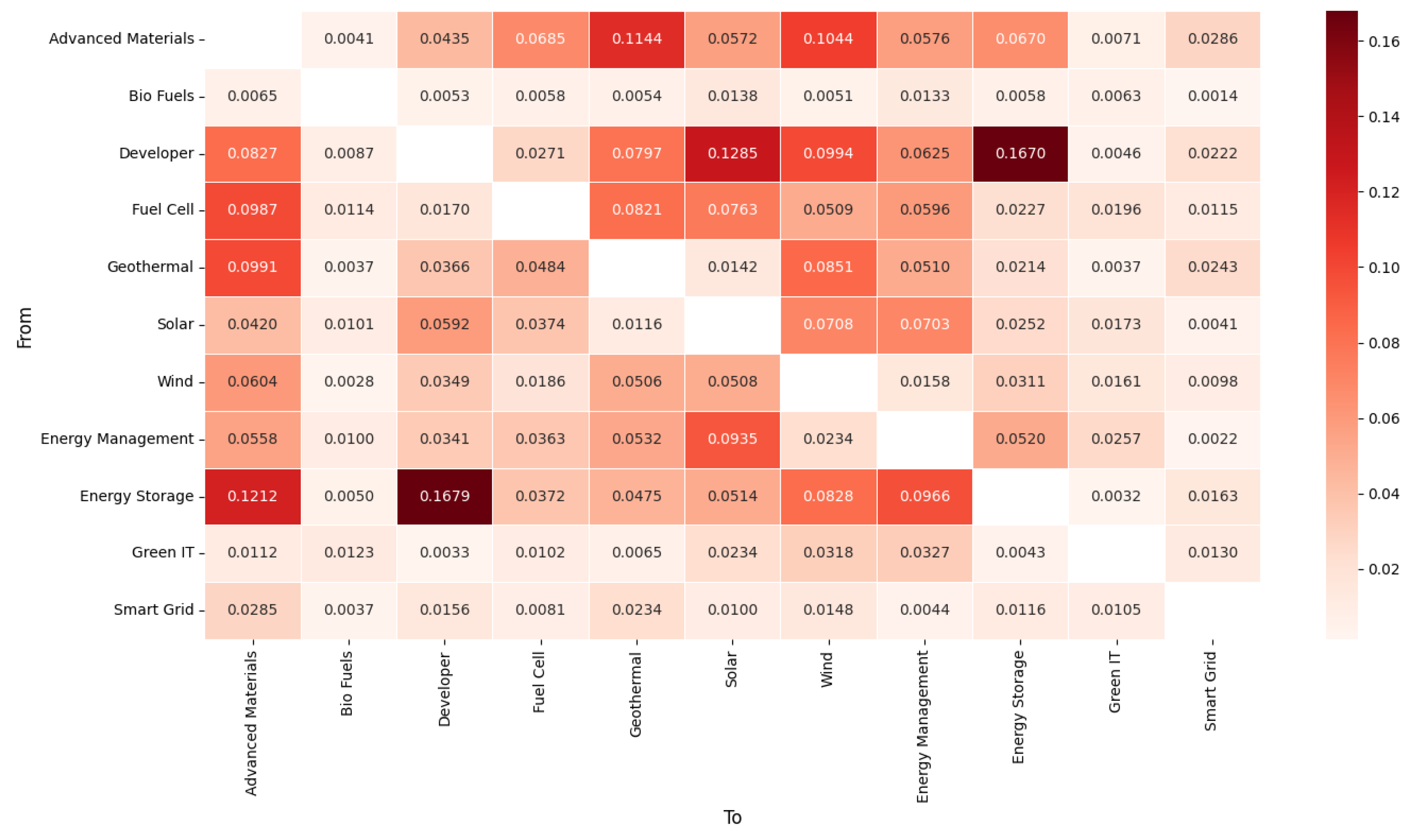
5.6. Risk-Spillover Level

Figure 4 shows the risk-spillover situation between 11 subindustry markets in the international clean energy market during the outbreak of systemic risk concentration. The values in the figure represent the mean of the conditional risk-spillover index, where columns represent risk emitters and rows represent risk receivers. Overall, during periods of systemic risk concentration and outbreak, the correlation between various markets significantly increases, and any risk event that occurs in one market may quickly spread to other markets. The advanced materials market, wind energy market, and solar energy market have played a leading role in risk transmission, and their risk contributions to other markets are particularly prominent.

From the analysis of spillover effects on various markets, the risk-spillover levels of the advanced materials market to the geothermal market and wind energy market are relatively high, at 0.1144 and 0.1044, respectively. The biofuel market has relatively low risk spillovers to other markets and risks received from other markets, which is consistent with the results of systemic vulnerability and systemic importance. This indicates that the biofuel market is in a relatively marginal position in the entire international clean energy system and is relatively stable.

The risk-spillover levels of the developer market to the solar energy market and energy storage market are relatively high, at 0.1285 and 0.1670, respectively. At the same time, the risk-spillover level of the energy storage market to the developer market is also relatively high, at 0.1679, indicating a highly correlated relationship between these two markets. In addition, the energy storage market, fuel cell market, geothermal market, and wind energy market all show high levels of risk spillover to the advanced materials market, with values of 0.1212, 0.0987, 0.0991, and 0.0604, respectively. The risk-spillover levels of the solar energy market to the wind energy market and energy management market are relatively high, at 0.0708 and 0.0703, respectively. The risk-spillover level of the energy management market to the solar energy market is relatively high, at 0.0935.

The developer market and solar energy market in the renewable energy market, as well as the energy management market and energy storage market in the energy efficiency market, further promote the risk transmission between the energy efficiency market and the renewable energy market. The high risk-spillover effects between the advanced materials market and multiple markets further demonstrate its vulnerability in the entire system.

Through the symmetry of the thermal matrix, the roles of various clean energy markets in tail risk shocks can be analyzed in depth. The upper triangle of the matrix displays the level of risk spillover received by each market, while the lower triangle reveals the degree of risk spillover emitted by each market. The analysis results show that the geothermal market, solar energy market, and wind energy market mainly play the role of net risk spillover in tail risk shocks, while the developer market and fuel cell market mainly play the role of net risk reception, which is consistent with the research results of Gong et al. (2023) [38].

Figure 5 shows the dynamic risk spillover between 11 subindustry markets in the international clean energy market during a period of systemic risk outbreak. Overall, during the period of concentrated systemic risk outbreaks, the level of systemic risk spillover in various subindustry markets fluctuated greatly. In 2015, the risk spillover was relatively concentrated, and the cumulative risk-spillover level in multiple subindustry markets was close to 1.8. After 2017, although risk spillover still exists, the volatility weakened compared to before, and the risk spillover in many subindustry markets decreased between 2018 and 2019, especially in the biofuel market, green IT market, and smart grid market. The reason for this is that the peak period in 2015 was related to changes in energy policies at the time, such as changes in global clean energy subsidy policies, significant fluctuations in oil prices, and intensified market volatility due to investment policies in renewable energy by various countries, leading to an increase in systemic risk spillovers. As the global energy market gradually stabilized after 2017, risk spillovers correspondingly decreased, indicating that policy stability and market maturity can help alleviate the transmission of systemic risks.

6. Conclusions

On the basis of considering the fat-tailed, time-varying, and asymmetric nature of financial returns, this study uses the dynamic factor copula model to establish a unified framework to examine the systemic risk of the international clean energy market from four dimensions: overall level of systemic risk, systemic vulnerability, systemic importance, and risk-spillover level. The Systemic Vulnerability Degree (SVD) and Systemic Importance Degree (SID) are introduced to analyze from the perspectives of systemic importance and systemic vulnerability, and a conditional risk-spillover index (CRSI) is constructed to measure the risk-spillover level between quantum industry markets. The research results are as follows.

First, based on the dynamic factor copula model, it was found that the interdependence structure between the 11 subindustries in the international clean energy market changes over time, and their correlation accumulates and increases during crisis events. This further confirms the findings of Naeem et al. (2020) [51] that major economic events or extreme conditions enhance connectivity between financial markets. In measuring the overall level of systemic risk, the joint probability of distress can identify changes in systemic risk in the international clean energy market.

Second, the systemic risks in the international clean energy market exhibit rapid and multiple outbreaks, and the joint probability of distress in the entire system can exceed 0.6. The outbreak of systemic risks is closely related to a series of major international events, demonstrating a strong correlation. This strengthens the understanding of Li et al. (2023) [53]; that is, under extreme market conditions, uncertainty will exacerbate the volatility of the clean energy market. Kuang (2021) [54] pointed out that the safe-haven nature of clean energy assets does not always play a full role in the global financial crisis or other major events, echoing the findings of this study. After the collapse of international oil prices in the second half of 2014, the level of systemic risk was significantly reduced. During the China–US trade war in 2018, COVID-19 in 2019, and the Russia–Ukraine conflict in 2022, the systemic risk had an upward trend.

Third, overall, the biofuel market has the lowest systemic vulnerability, while the advanced materials market has the highest systemic vulnerability. At different times, the ranking of systemic vulnerability in subindustry markets also varies. In the measurement of systemic importance, the energy efficiency market has the highest systemic importance. This conclusion is consistent with the findings of Zhao et al. (2024) [7], which shows that the systemic importance of the energy management market and the energy storage market continues to be significant, and the correlation with other markets is strong, which has a $“$ripple effect” on the entire international clean energy system.

Finally, during the period of systemic risk concentration and outbreak, the correlation between various subindustry markets significantly increases, and any risk event that occurs in one market may quickly spread to other markets. The advanced materials market and renewable energy market play a dominant role in the risk contribution to other markets, especially the geothermal market, solar energy market, and wind energy market, which are net risk overflow parties in tail risk shocks, while the developer market and fuel cell market are net risk receivers.

It should be emphasized that the research has certain limitations, which in turn indicate possible future research directions.

First, this study mainly focuses on the correlation between subindustry markets in the clean energy market. However, it has not been further deepened to the microenterprise level under the subindustry market. Therefore, future research can explore the risk tolerance of enterprises and reveal the role of individual institutions in the clean energy market system. Second, there is a lack of comprehensive and detailed analysis of how the external shock events conduct and affect the path of systemic risk in the clean energy market through specific mechanisms. Therefore, in the future, we can explore the transmission path of different types of external shock events (such as climate change and policy change) to systemic risk. Finally, the potential driving factors (such as macroeconomic changes, market sentiment fluctuations, etc.) of the abnormal rise of systemic risk levels during nonimpact events have not been fully revealed in this study, which may limit the comprehensive understanding of risk triggers.