An Exploration of Groundwater Resource Ecosystem Service Sustainability: A System Dynamics Case Study in Texas, USA

Abstract

Groundwater, a crucial natural resource on a global scale, plays a significant role in Texas, impacting various essential ecosystem services either directly or indirectly. Despite efforts of state- and community-level regulations and conservation efforts, there is an ongoing trend of declining groundwater levels in the state of Texas. In this study, we utilized the systems thinking and system dynamics modeling approach to better understand this problem and investigate possible leverage points to achieve more sustainable groundwater resource levels. After conceptualizing a causal loop diagram (CLD) of the underlying feedback structure of the issue (informed by the existing literature), a small system dynamics (SD) model was developed to connect the feedback factors identified in the CLD to the stocks (groundwater level) and flows (recharge rate and groundwater pumping) that steer the behaviors of groundwater systems across time. After completing model assessment, experimental simulations were conducted to evaluate the current state relative to simulated treatments for improved irrigation efficiency, restricted pumping rates, cooperative conservation protocols among users, and combination strategy (of all treatments above) in the long-term. Results showed that groundwater stress (and the associated repercussions on related ecosystem service) could be alleviated with a combination strategy, albeit without complete groundwater level recovery.

1. Introduction

Groundwater is stored water beneath the surface, moving slowly through layers of soil, gravel, and rock which acts as filters as it transits voided pore space until it reaches the saturated zone (hereafter called aquifer or groundwater) [1]. Aquifers play a tremendous role as a source of freshwater-derived ecosystem services, including but not limited to irrigation for agriculture, sources for human consumption and sustaining populations, and supporting multitude environmental and ecological functions [2,3]. These ecosystem services are threatened in many arid- to semi-arid regions (e.g., most of Texas, USA) by the reduction in groundwater storage, loss of surface water–groundwater connectivity, and groundwater quality impairment via leaching surface contaminants into aquifers [2]. Increasing drought severity (which may become more pronounced with climate change) can lead to higher extraction rates, which coupled together contributes to more rapid groundwater level declines in drier years, highlighting the vulnerability of groundwater systems to a changing climate [4].

To date, much groundwater modeling work has been done to model specific aquifer systems at fine spatial scales and with extreme specificity of hydrogeologic processes (sometimes with or without socio-economic feedbacks or incorporation of ecosystem services concepts). Here, we employ the systems thinking and system dynamics (SD) modeling approach to problem solving [5] with use of a small SD groundwater model to explore possible management or policy leverage points which could directly improve groundwater resource conservation and by extension the diversity of ecosystem services it provides and supports. This paper proceeds as follows. First, we review how groundwater resources provide or support the delivery of ecosystem services. Then, we describe the systems thinking approach we employed to understand the groundwater-ecosystem service nexus in our case study region, Texas USA. A small SD model is then outlined which captures the core stock-flow structure and resulting behavior patterns observed in groundwater systems of interest (similar to [6]). The model is tested for a variety of scenarios which we discuss and link back to the impacts to ecosystem service demands arising from society and the environment. We close with recommendations for future work.

2. Ecosystem Services of Groundwater Aquifer Systems

Ground water is one of the most important natural resources globally which directly or indirectly influences a range of critical ecosystem services: provisions, regulating, supporting, and cultural (classical ecosystem service categories defined in [7]). In this section, we review important groundwater ecosystem services studies to inform the context of our model and frame discussion of our results. Because the relevant literature pertaining to groundwater ecosystem services for any one particular aquifer in Texas is lacking, our review is more global in scope in order to capture the best available literature in each category. Although the studies cited may not be directly transferrable or other geographic areas due to differences in location (geology, landscape position, etc.), research scales, and methodologies, they do offer some insight into the possible range of ecosystem services offered by groundwater systems that necessitate further reflection when considering policy and management trade-offs.

2.1. Groundwater and Provisioning Services

Groundwater provides a reliable source of irrigation water for agriculture given that groundwater-irrigated lands consume about 38–43% of total consumptive water use for global food and fiber production [8,9,10] or available calories [11]. Because of the high value of agricultural production supported by irrigation, governments often support increases in investments in irrigation efficiency in effort to improve the “crop per drop” [11].

Groundwater risk indices show that groundwater losses are highly dependent on governance structure and food security needs and as such, mitigation strategies should seek reliable water transfers via agricultural trade rather than exploiting finite water resources for short-term food sufficiency locally [12]. In addition, groundwater risks are closely linked to other environmental externalities associated with agricultural land conversion given the direct relationship of land use to other food security and environmental concerns [13].

Multiple lines of evidence from varying regions suggest contradictory policy recommendations about groundwater management. For example, some suggest saving water today will result in increased net production due to projected future increases in crop water use efficiencies [14] while others suggest that economic benefits of irrigation will continue to outweigh its costs and therefore certain regions will be better suited for long-term investments in groundwater pumping [15] despite its common good characteristics. In regions where pumping exceeds groundwater recharge (e.g., Texas High Plains), suggested recommendations without changing irrigated surface area include (but are not limited to): (1) increasing weather-based irrigation scheduling; (2) converting gravity-irrigated land to center pivot irrigation; and (3) replacing high-water demand crops with less water-intensive crops [16].

Given the importance of groundwater to provisioning services, there continues to be a need to increase science-based education and extension programming on integrated approaches that emphasize both irrigation technology and the best management practices [6]. As concerns increase when crop yield reductions occur, risks associated with changing management practices, and costs of technology adoption and maintenance remain barriers to adopting water conservation practices [17].

2.2. Groundwater and Regulating and Supporting Services

Groundwater plays a critical link in the maintenance of regulating ecosystem services such as water quality regulation, reclamation, flood prevention, and climate regulation. Recharge from heavy rainfalls and floods can cause contamination of shallow aquifers, and thus can seriously impact groundwater quality [4]. Moderate increases in aquifer temperature [+5 to 10 °C] generally causes minor changes in water chemistry, microbial biodiversity, and ecosystem function in non-contaminated and energy-poor (oligotrophic) groundwater systems, while aquifers at temperatures ≥ 30 °C contaminated with organics, nutrients, and heavy metals (e.g., urban areas) or with intensive land use (e.g., agriculture), significant changes in water quality and ecological patterns are expected [18]. Consequently, holistic management which addresses multiple heat sources is needed to balance potential conflict between groundwater quality for drinking and groundwater as an energy source or storage media for geothermal systems [19]. In addition, the time since groundwater was recharged (i.e., groundwater age) can be important for various geologic processes, such as chemical weathering and coastal waters eutrophication [20,21].

Ecosystem services linked to freshwater resource management (e.g., flood control, the provision of hydropower), as well as carbon storage and sequestration have received increasing scientific and on-the-ground attention by managers and policy makers [22]. Reconciling increasing ecosystem service demands from society with finite freshwater resources remains one of the great policy dilemmas [8] given the role of the hydrologic cycle in global nutrient cycling (e.g., C, [22]) and the fact that approximately 99% of Earth’s freshwater resides in aquifers [23]. Studies in highly developed watersheds mixed with agriculture and urban development have found that water quality policies can be leveraged to protect other ecosystem services such as freshwater storage and flood regulation [24]. Phreatic ecosystems (saturated groundwater ecosystems in porous and fractured-rock aquifers) are research frontiers for freshwater ecology [25,26].

2.3. Groundwater and Cultural Services

The least studied or understood bundle of groundwater ecosystem services relate cultural ecosystem services. Previous investigators have highlighted the gap and determined the source of misunderstanding to the inadequate integration of social science and ethical factors with the environmental sciences [27]. The field of sociohydrology has developed to explore human and hydrological system connectivity and feedbacks [28] with particular interest on the social-cultural roles and relationships pertaining to the evolution of basin-scale allocation patterns and public participation in water management policies [29].

Within the context of Texas and the southwestern U.S., sociohydrologic research has studied specific cases ranging from strategic trade-offs of water conservation policy in Austin, Texas [30] to cultural continuity and community mutualism in New Mexico acequia communities [31,32,33].

3. Systems Thinking Case Study: Groundwater in Texas, USA

Using the Iceberg Diagram concept in systems thinking [34], we aimed to better understand the drivers and feedback dynamics that influence groundwater systems in Texas. The Iceberg begins with event-level descriptions of the problem followed by characterization of the trends and patterns over time in important variables associated with the problem. After capturing the event-level issues (what has happened?) and analyzing temporal trends and patterns (what has been happening?), the underlying structure of the problem is then constructed in terms of feedback loop and delays in order to understand why the situation has unfolded the way it has (why has it been happening?). This feedback structure is often presented in the form of a conceptual model called a causal loop diagram (or CLD). Important mental models of stakeholders are also recognized to better appreciate the diverse perspectives of all stakeholders involved. Mental models are the relationships and assumptions about the worlds held in a person’s mind, which are influenced by past experiences and knowledge and which influence how we perceive and interact the world around us [35]. This Iceberg Diagram methodology has been widely used in many contexts and is applicable as a first step to studying complex problems across domains and problem contexts [34]. In this section, we follow the Iceberg Diagram method to better understand the Texas groundwater problem and contextualize the model.

3.1. What Has Happened? Event-Level Description

The Texas landscape overlies 26 aquifer formations, eight of which reside under the majority of the surface area of the state and are considered major aquifers: Seymour alluvium, Ogallala, Hueco-Mesilla, Gulf Coast, Carrizo-Wilcox, Edwards-Trinity Plateau, Edwards Balcones Fault Zone, and Trinity aquifer [36,37]. Across the state, groundwater is currently being lost 6.5 times faster than the average recharge rate [38,39]. At this rate, groundwater reductions will continue to increase in the future, which has implications for land subsidence issues, depletion of springs and their contribution to aquatic/riverine habitat maintenance, and increasing financial costs for agriculture and municipal use [40].

Several primary factors are interacting which drive the current groundwater stress being observed throughout the state:

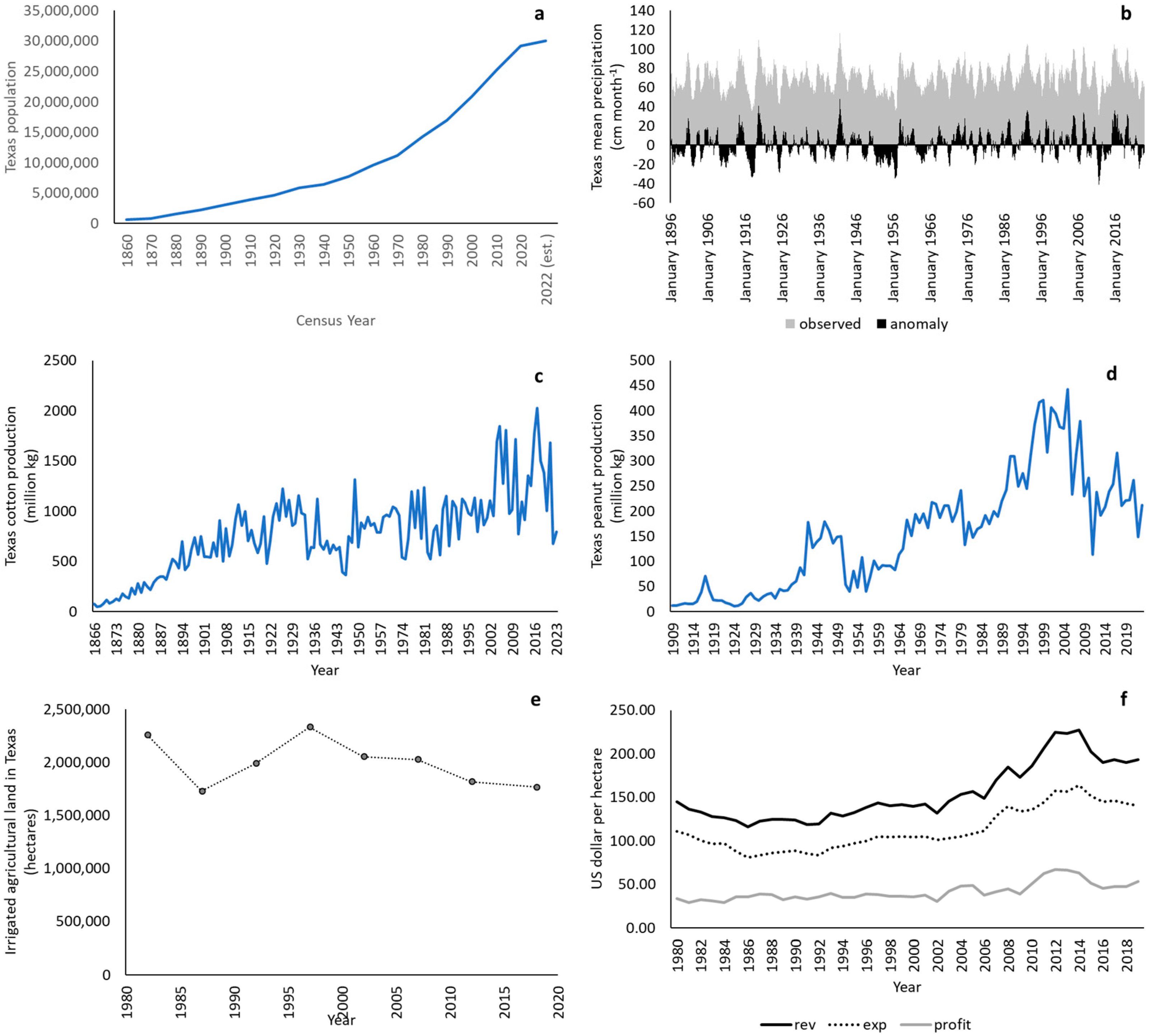
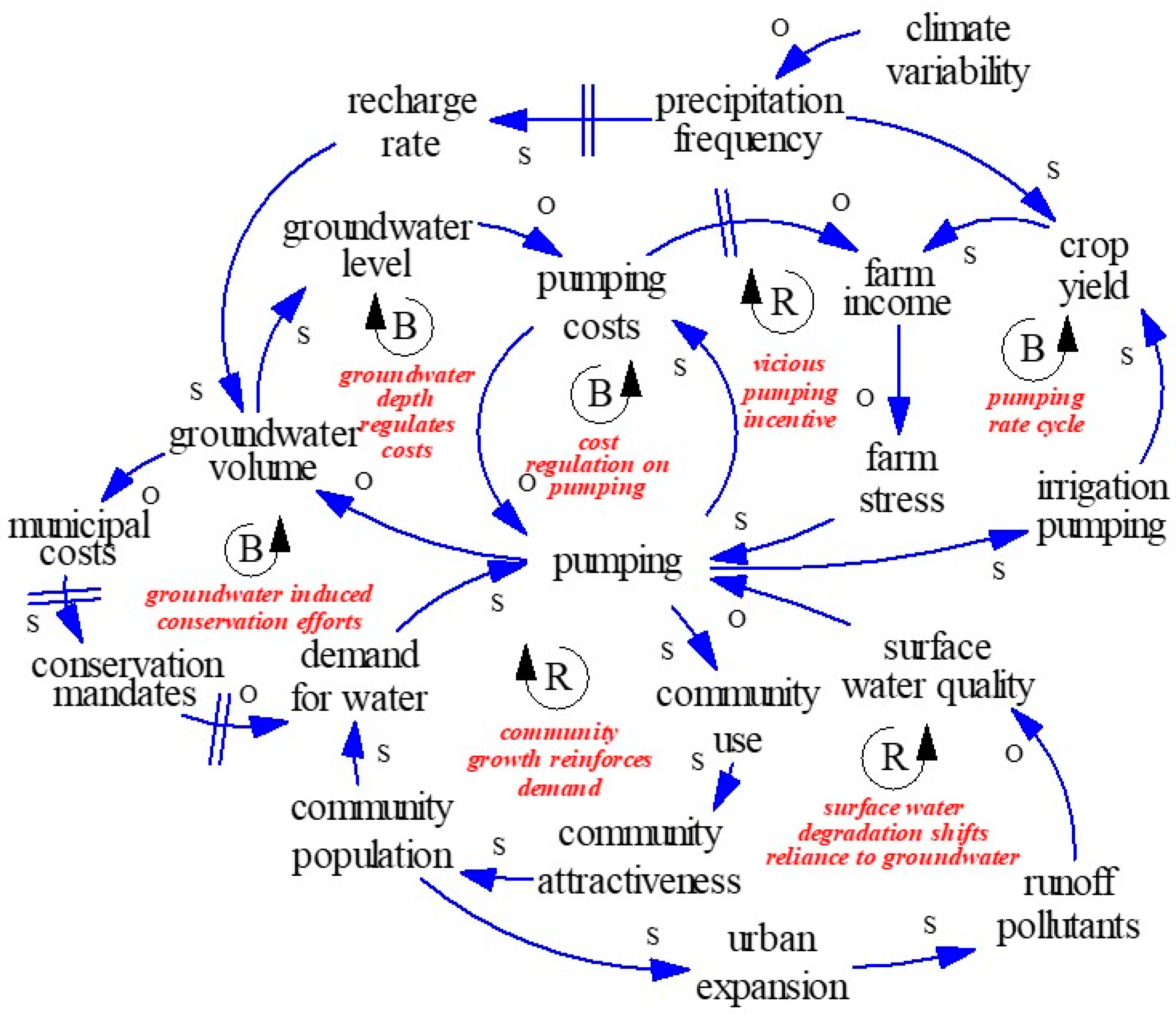
• Urbanization: As communities and population centers grow, the more it becomes appealing for others (both in and out-of-state) to relocate to these areas; as the population within that community grows, so does the need for water supply. With increased urbanization, communities relying on surface water supplies are more susceptible to water quality issues arising from nutrient and runoff pollutants that affect water quality and treatment costs, which in turn incentives cities to acquire groundwater rights to fulfil their water demands. This issue will not be going away as long as the population in Texas continues growing relative to available water supply [41]. In areas with a higher population, greater pumping rates have led to higher costs (due to groundwater level reductions) and the likelihood of externalities such as groundwater contamination or land subsidence is greater [42,43].
• Agriculture: Farmers rely heavily on groundwater for their farms, this allows the farm to generate income, which itself depends on crop yield, that irrigation supports [44]. However, farms experiencing severe stress from either drought (climate variability), productivity (soil degradation), revenue (crop yields and/or quality), or combinations thereof can hit farmers very hard financially, which may incentivize accelerated irrigation pumping as a coping or recovery strategy but lead to increased pumping costs.

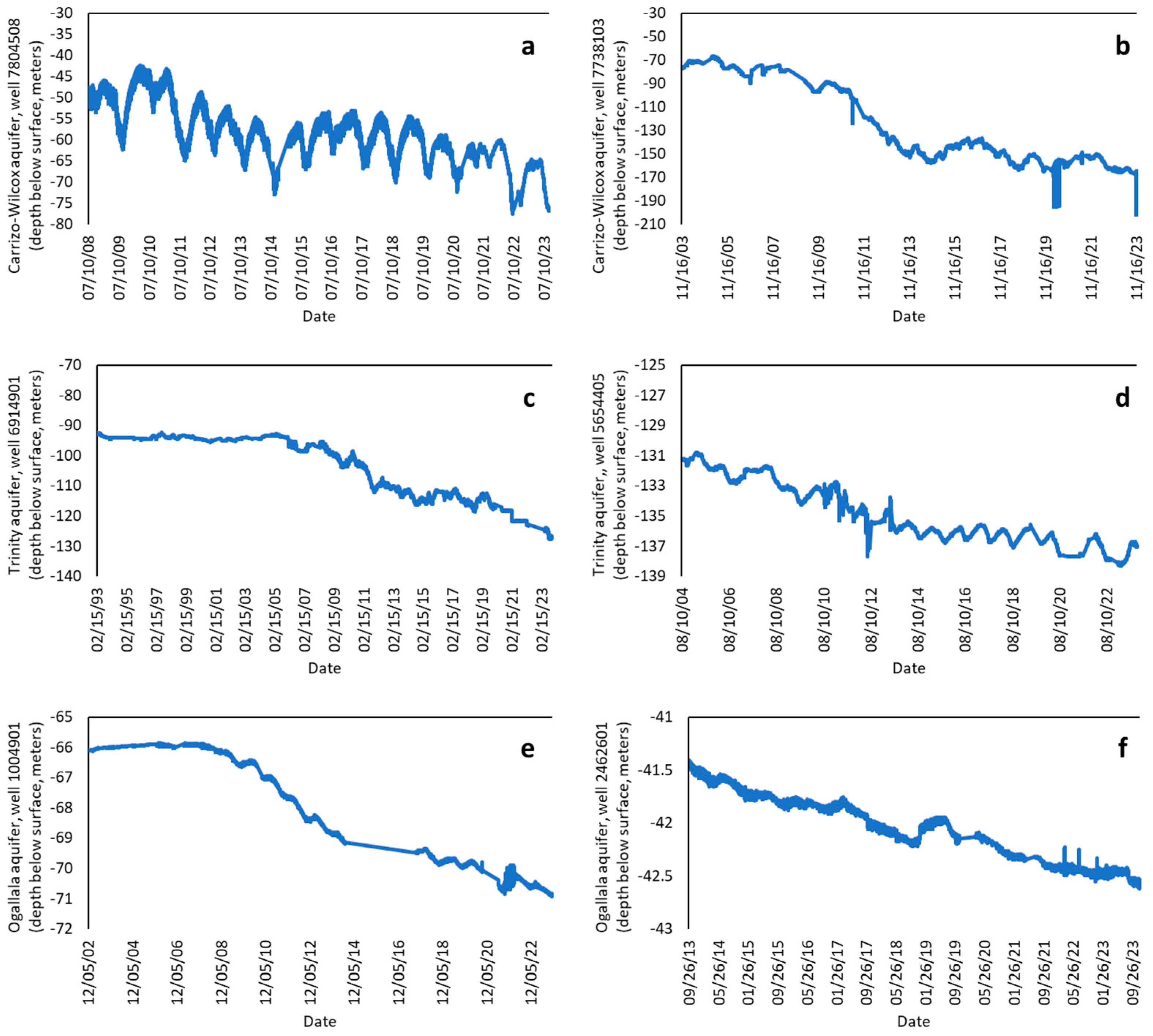
3.2. What Has Been Happening? Trends and Patterns over Time

Based on this event-level understanding, we recognized several important interacting variables that could further enhance our understanding of the problem when analyzed over time. These variables were: aquifer levels, precipitation, population, agricultural yields and incomes, irrigation and/or pumping (rates and costs), and water quality. Publicly accessible data were available from the Texas Water Development Board (TWDB) for aquifer levels [45], National Oceanic and Atmospheric Association (NOAA) for precipitation [46], United States Census Bureau for population [47], and United States Department of Agriculture (USDA) for agricultural yields, incomes, and pumping rates [48]. For those variables without publicly available data, we discussed possible trends and patterns over time given current anecdotal evidence from local stakeholders in Texas [49].

Generally, several important temporal insights emerge. Regardless of location or aquifer in question, groundwater levels have tended to decline [44,50] (Figure 1). During this same time period, the Texas population has grown at increasing rate (Figure 2a). Meanwhile, mean annual precipitation has been stable (albeit with cyclical drought and wet cycles; Figure 2b), with the eastern side of the state being 10–15% wetter and the western side of the state experiencing no change in precipitation or being up to 6% drier over the past 140 years [46]. In addition, and given the negligible long-term change in mean precipitation, precipitation frequency has shifted over time to less smaller showers and more but fewer larger downpours, indicated by the increase in the number of precipitation events greater than 7.2 cm (or three inches; [51]). Agriculturally speaking, while irrigated crop yields have grown (Figure 2c,d), irrigation rates have remained relatively constant (Figure 2e) (indicating increasing water use efficiency). While crop yields have had positive impacts on farm revenues, increasing operating costs have led to agricultural incomes being either stable or declining (Figure 2f).

Based on the above trends and patterns (Figure 1 and Figure 2) as well as anecdotal evidence from stakeholders, we also inferred the trends and patterns of other variables that were difficult to quantify. For example, with operating productivity increasing but with incomes either stagnant or declining, we inferred that farm stress has risen over time. Because crop yield potential has risen over time with improved crop genetics, we inferred demand for water by farmers in the agricultural sector has risen with the goal of minimizing crop yield gaps. Likewise, growth in the total population has led to growth in demand for water by the municipal and industrial sectors. With these stresses to groundwater systems, conservation efforts of state and community leaders have escalated in the form of conservation mandates or pumping restrictions (in the short-term) or establishment of groundwater conservation districts (in the long-term) [54].

3.3. Why Has It Been Happening? Causal Feedback Structure and Stakeholder Mental Models

After reading and reviewing articles describing the contemporary nature of the problem and examining important trends and patterns over time, we developed the following focusing question to guide our conceptual causal loop diagram (CLD) development of the underlying feedback structure of the problem: if we know groundwater is a limited resource that must be managed, why are water tables continuing to decline?

While groundwater levels are a function of precipitation (total water volume reaching the land surface), recharge (the amount of surface water which escapes runoff into streamflow, storage in soil, depression, or reservoirs, or used consumptively by organisms and proceeds below the vadose zone into groundwater), current groundwater storage and capacity and weather patterns; a main contributor is excessive pumping [55]. To illustrate the underlying structure of interconnected feedbacks which are driving the groundwater depletion in Texas, we developed a conceptual model or CLD. In a CLD, links between variables describe the direction of influence between two variables—a cause and an effect. If an increase (or decrease) in the cause variables leads to a subsequent increase (or decrease) in effect variable, the link is labeled as a S link (i.e., they move in the same direction). For example, the link from precipitation frequency to recharge is a S (same) link meaning that as precipitation frequency increases then recharge will also increase (all other things being equal). If a decrease (or increase) in the cause variable leads to a subsequent increase (or decrease) in the effect variable, the link is labeled an O link (i.e., they move in opposite directions). For example, the link from climate variability to precipitation frequency is an O (opposite) link meaning that as climate variability increases precipitation frequency decreases. Delays, when significant time is required between cause and effect, are shown on a link as a hash-mark between variables. For example, it takes time for water to move from precipitation through the surface before eventually becoming actual recharge into groundwater.

We identified seven feedback loops in our CLD which were labeled as either reinforcing (R) loops, where increases (decreases) in one variable eventually feeds back on itself creating subsequent increases (decreases), or balancing (B) loops, where increases (decreases) in one variable eventually feeds back on itself leading to a decrease (increase) in itself, stabilizing the original perturbation (all other things being equal). These six feedback loops help explain why over time people have become reliant on groundwater pumping despite the fact that continued pumping has led to higher pumping costs and lower groundwater levels (Figure 3).

As farm stress and demand for water increases, pumping increases, which draws down the groundwater volume and therefore water table level. As groundwater levels drop, pumping costs increase (B-loop named “groundwater depth regulates costs”), thus, slowing the rate of pumping in the short-term (B-loop named “cost regulation on pumping” whereby pumping is reduced due to increased costs and/or pumping rate restrictions). In the long-term, greater pumping costs erode farm income, leading to greater farm stress (R-loop named “vicious pumping cycle”). With greater stress, farmers cope with pumping more water for irrigation (or buying-out neighboring water rights) in attempts to increase crop yields, aimed at restoring farm income (B-loop named “pumping rate cycle”). With greater income, farm stress goes down (meaning farmers worry less given the most recent yield and profit outcomes), which feeds back to their pumping decisions (greater profitability, less reason for increasing pumping).

Pumping is also influenced by population growth and use for human consumption as communities grow. This creates a community attractiveness for people to relocate to population centers given the benefits of water use. While this happens, population rises and so does the demand for water, which feeds back into excessive pumping creating a reinforcing loop (R-loop named “community growth reinforces demand”).

As population growth fuels urban expansion, runoff pollutants increase and deteriorates water supplies (and associated treatment costs). Decreasing quality of available surface water reinforces desire for and reliance on pumping groundwater to fulfill societal needs (R-loop named “surface water degradation shifts reliance to groundwater”). Finally, as pumping draws down groundwater levels and municipal costs increase, policy leaders have implemented a variety of conservation mandates, which spurs conservation effort to decrease demand for water and therefore pumping activity (B-loop named “groundwater induced conservation efforts”).

One example of conservation mandate efforts was the creation of groundwater conservation districts (GCDs) by the Texas legislature. Managers of GCD’s must develop plans to preserve safe water supplies to be available for future generations, including record keeping of water well drilling and closure activities, including approval for new wells as well as approval of the timing and amount of pumping by water rights holders [56]. The goal of GCDs has been to create increased cooperation and active participation among water users and their communities, deployment of real-time monitoring networks, and to reinforce scientific support to achieve sustainable groundwater management to help reverse declining aquifer levels in the state. Despite these efforts, groundwater levels continue to decline (Figure 1).

The main stakeholders we have distinguished in this study were farmers, municipal leaders, residents, and industry in population centers, and managers of GCDs. Based on previous research which interviewed various stakeholders in south Texas regarding water source and quality issues [49], we were able to describe stakeholder mental models using a collection of quotations which shed light on the prevailing perspectives of groundwater users:

• Agriculture: The farmers and ranchers view the situation as they must sustain or improve yield to survive. If they “get more rain, we won’t have to pump more”, but when they are particularly stressed during short-term droughts “I need more water so I pump”. Although they recognized climate variability to be a significant driver (“We need more rain”), it has not been clear if agricultural users recognized how irrigation decisions influence costs as well as yields (“Pumping costs keep rising… we simply need more water”).
• Municipalities (both domestic and industrial users): Likewise, community stakeholders stressed the “need for water to survive and [continue to] grow”. Although groundwater comes at a significant cost, municipal stakeholders recognized another cost factor influencing their water sourcing decisions, namely treatment costs stemming from surface water quality degradation (“We need clean water… becoming more and more important to manage costs of water”).
• Groundwater conservation districts: The GCD managers saw the cycle (or throughput) of water through manmade systems must slow down before groundwater become so scarce it becomes essentially “lost” to productive use, given “accelerated reliance on pumping [by all users] is affecting the amount of water available”. In addition, groundwater quality is growing in concern given “more pollutants in runoff” and “nutrient concentration issues with declining water tables”, especially salts. Lastly GCD managers had a noticeable appreciation for the regulatory mechanisms or constraints on conservation effort implementation, given “not all of the state is in a GCD, some aquifers have multiple GCDs while others have none, and conservation emphasis varies greatly between GCD... in Texas, surface rights holders have a strong legal right to use groundwater [which makes voluntary conservation difficult]”.

After examining the major events, trends, and underlying feedback structures of the declining groundwater problem, we transitioned our investigation to developing a small SD model of groundwater systems capable of linking the recognized factors above to the physical stock and flows which drive groundwater level behaviors over time.

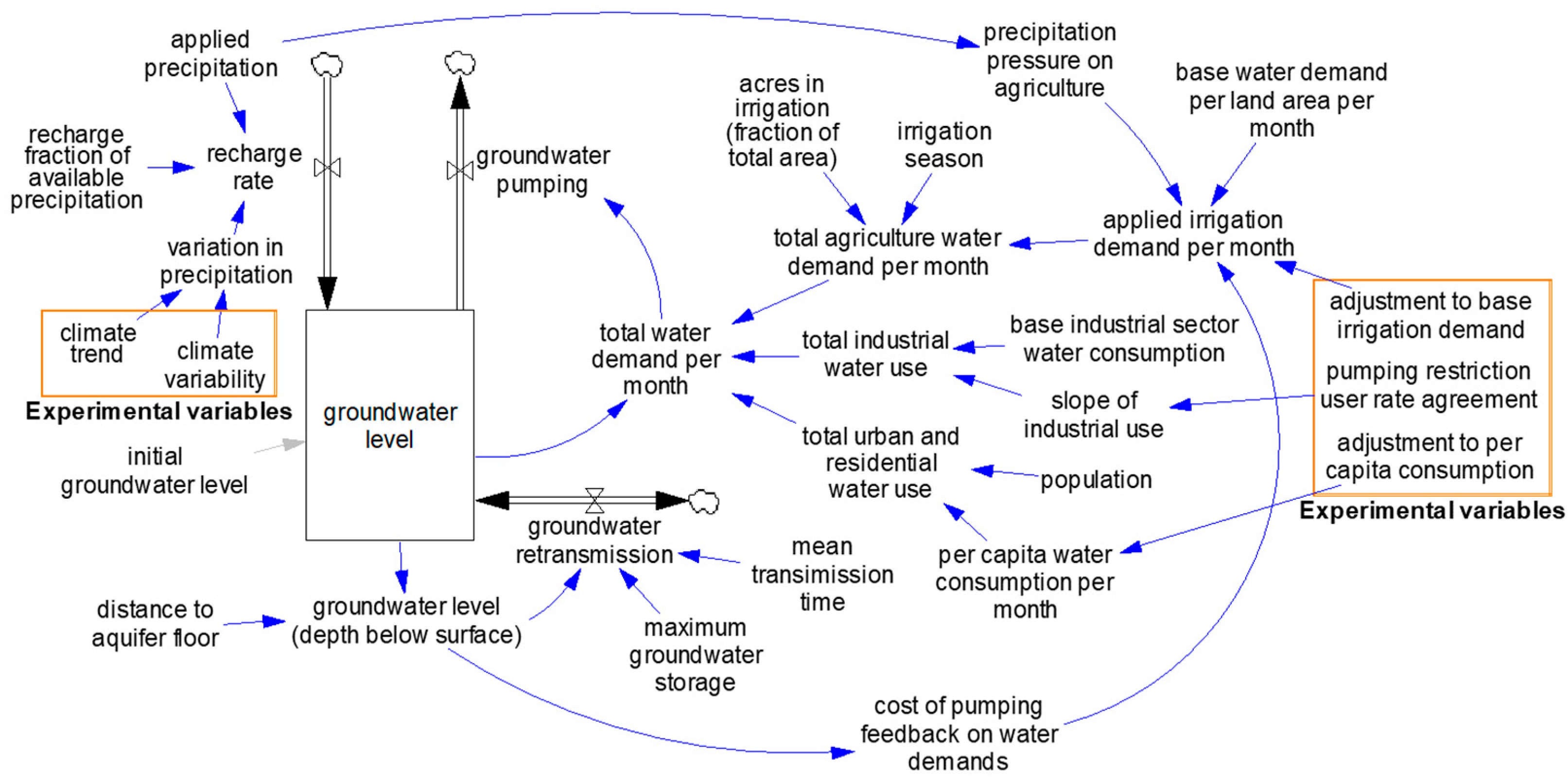
4. System Dynamics Model Application

4.1. Model Overview

The SD approach is the science of feedback behavior in complex systems and a philosophy for the structure of systems by which to relate structure to behavior [6,57]. The SD methodology utilizes computer models to generate the behavior of a system or problem of interest via simulation [35,58]. An SD simulation model is constituted by “building blocks” of stocks (or levels) and flows (or rates of change over time) [57], whereby stocks are “quantities in specific locations or conditions in a system” which “accumulates or drains over time” and “can only be changed by flows” [35]. Flows which change stocks “represent activity, in contrast to stocks, which represent the state of the system” and can be defined as the movement of quantities into and out of stocks (within a model boundary) or into and out of sources and sinks at the model boundary [35]. All SD models include stocks and flows as these are the philosophical starting point for determining real-world dynamics [57]. In this case, the level or stock of interest is the amount of water in groundwater, with inflows from recharge and outflows from groundwater pumping (vertical flows) as well as groundwater retransmission, which could be an inflow or outflow (horizontal) depending on the level of water (i.e., if the groundwater level is at its storage capacity, new recharge will displace storage via retransmission out of the aquifer horizontally; if the groundwater level is below its storage capacity, it can be recharged via both surface water infiltration as well as horizontal retransmission due to head level difference). The model (Figure 4) was constructed in the Vensim^TM modeling environment (Ventana Systems Inc., Harvard, MA, USA) [59] using SD. The model employs a time unit of one month, time horizon of 360 months or 30 years, and time-step of 0.25 months (

Table 1. Model overview and time parameters.

Dimension	Description
Model boundary	Groundwater, its flows, and how groundwater level feeds back to influence future flows (endogenous) Precipitation, population, and irrigation and industrial demand (exogenous) Population and economics and policy feedback processes (excluded)
Key variables	Groundwater level, recharge rate, groundwater pumping, cost of pumping feedback on water demands
Time parameters	Time unit = 1 month, Time-step = 0.25 months, Time horizon = 360 months

). Here, we strived for a small model structure (e.g., one stock variable) capable of a diversity of dynamics relative to more complex groundwater models (e.g., many stocks) that aim to preserve real-world data replication to a particular case [60,61].

The primary model stock was groundwater level (Figure 4; Equation (1)), given an initial groundwater level (Equation (2)). This was converted to groundwater depth level (depth below surface) given the distance to aquifer floor (Equation (3)). Groundwater retransmission into or out of the groundwater stock occurred depending on the depth below surface—if the depth was shallower than the surrounding retransmission aquifer head level, water was retransmitted as an outflow, if the depth was deeper than the surrounding retransmission aquifer head level, water was retransmitted as an inflow (Equation (4)), subject to constraints on maximum groundwater flow rate and transmission times (Equations (5) and (6)).

The recharge rate (Equation (7)) was a function of rainfall applied and the recharge fraction of available precipitation (Equation (8)). Rainfall applied was formulated as a deterministic stochastic function of normally distributed precipitation depths arriving at Poisson distributed precipitation arrival times (see Turner and Kodali [62] and Laio et al. [63] for detailed model methodology for precipitation modeling, which is outside the scope of this paper).

The groundwater pumping outflow (Equation (9)) aimed to capture the cumulative pumping activity from agriculture, municipal and industrial uses.

Total agriculture demand per month (Equation (10)) was the product of acres in irrigation (fraction of total surface area) (Equation (11)), applied irrigation demand per month (Equation (12)), and irrigation season (a binary switch where 1 indicated active pumping during the growing season March to October and 0 indicated fallow period October to March which excluded irrigation). Applied irrigation demand per month was regulated by the base water demand per land area per month (0.3048 m/ha/month; Equation (13)), precipitation pressure on agriculture (Equation (14)), and cost of pumping feedback on water demand (Equation (15)). Precipitation pressure on agriculture, calculated as the mean precipitation divided by the precipitation trend, captured how changing precipitation trends may influence demand for irrigation (i.e., when precipitation increases, less irrigation demand needs to be filled, when precipitation decreases, irrigation demand rises in attempt to meet all base water demands per unit area; Equation (12)). Cost of pumping was formulated as a lookup or table function such that when depth to groundwater increased (decreased) costs of pumping increased (decreased). This then fed back to reduce (elevate) irrigation demand per as groundwater became less (more) easily accessible from the surface.

Total industrial use (Equation (16)) was the product of base industrial sector water consumption (Equation (17)) and the slope of industrial use (representing the growth in industry over time), which increases over time based on assumed growth rate (Equation (18)).

Total urban and residential water use (Equation (19)) was the product of population (Equation (20)) multiplied by per capita water consumption per month (Equation (21)). A summary of model equations listed above is provided in

Table 2. Summary list of model equations and parameters constituting the core structure of the groundwater model. Types of variables include stock (levels or integration), flows (rates or fluxes per unit time), and auxiliary variables (parameter values or functions). Units of ‘dmnl’ refer to dimensionless units (i.e., ratios or fractions). Conditional statements are read “IF (condition) THEN (function if condition is true) ELSE (function if condition is false)”. The LOOKUP or table function provides a list of input variable (x) and output variable (y) coordinates. The notation * represents a multiplication function or product between two variables.

Variable or Parameter	Type	Equation or Parameter Value	Equation in Text	Unit
Groundwater level	stock	=INTEG (recharge rate-groundwater pumping-groundwater retransmission)	(1)	m
Initial groundwater level (depth below surface)	aux	150 1	(2)	m
Distance to aquifer floor	aux	300 2	(3)	m
Groundwater retransmission	flow	IF (groundwater level > max groundwater storage), THEN (groundwater level-max groundwater storage)/mean transmission time, ELSE (-groundwater inflow)	(4)	m/month
Maximum groundwater flow rate	aux	0.03 3	(5)	m/month
Mean transmission time	aux	1/30 3	(6)	month
Recharge rate	flow	rainfall applied * recharge fraction of available precip	(7)	m/month
Recharge fraction of available precip	aux	0.037 4	(8)	dmnl
Groundwater pumping	flow	adjusted water demand per month	(9)	m/month
Agriculture demand per month	aux	“acres in irrigation (fraction of total area)” * applied irrigation demand per month*irrigation season	(10)	m/month
Acres in irrigation (fraction of total area)	aux	0.75 5	(11)	dmnl
Applied irrigation demand per month	aux	base water demand per land area per month * cost of pumping feedback on water demands * precipitation pressure on agriculture	(12)	m/ha/month
Base water demand per land area per month	aux	0.3048 5	(13)	m/ha/month
Precipitation pressure on agriculture	aux	mean precipitation/precipitation trend	(14)	dmnl
Cost of pumping feedback on water demand	aux	LOOKUP (“groundwater level (depth below surface)”, ([(−750,0)–(0,2)], (−750,0.5), (−500,1), (0,2))	(15)	dmnl
Total industrial use	aux	base industrial sector demand + RAMP(slope of industrial use, INITIAL TIME, FINAL TIME)	(16)	m/month
Base industrial sector demand	aux	0.05 3	(17)	m/month
Slope of industrial use	aux	0.006 3	(18)	dmnl/month
Total urban and residential water use	aux	Population ratio to initial * per capita water consumption per month	(19)	m/month
Population ratio to initial	aux	1 + RAMP(0.003, INITIAL TIME, FINAL TIME)	(20)	dmnl
Per capita water consumption per month	aux	0.025 6	(21)	m/month

¹ Initial aquifer level based on range of values observed in Texas, USA. ² Assumed value for testing purposes to check for internal consistency of model structure (e.g., conservation of mass) when model values approach thresholds (e.g., distance to water becomes prohibitive of use as a natural resource). ³ hand calibrated value for the behavior reproduction test. ⁴ recharge values vary based on water depth and soil type, and average values range from around 1% of precipitation in the Texas High Plains region to 7% in wetter climates with sandier soils. Model recharge rate reflects an average of possible values across the state. ⁵ hand calibrated value for the behavior reproduction test, percentages reflect the amount of land represented in irrigated agricultural areas reliant on groundwater (e.g., Texas Wintergarden, Texas High Plains, etc.) and their approximate crop irrigation allocation based on common Texas crops (e.g., cotton, sorghum, maize, among others). ⁶ calibrated consumption based on Texas population of 30 million, total Texas surface area of 6.956 × 10¹¹ m, and average consumption per person per month of approximately 11 cubic meters, equates to roughly 2.5 cm depth (or 0.025 m) consumed per person per month.

(additional information about model relationships and the assessment and calibration process which follows in 4.2 can be found in Appendix A).

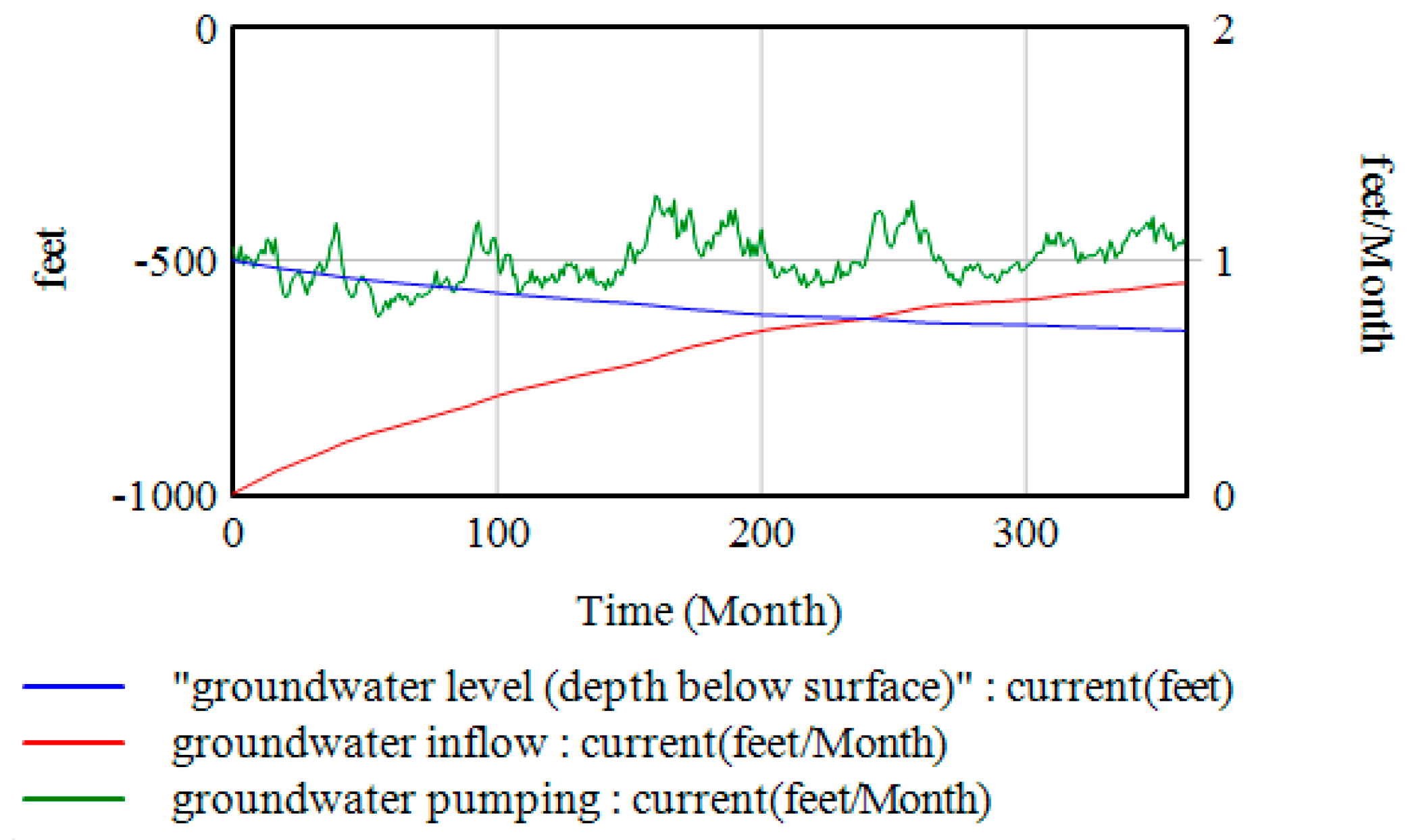
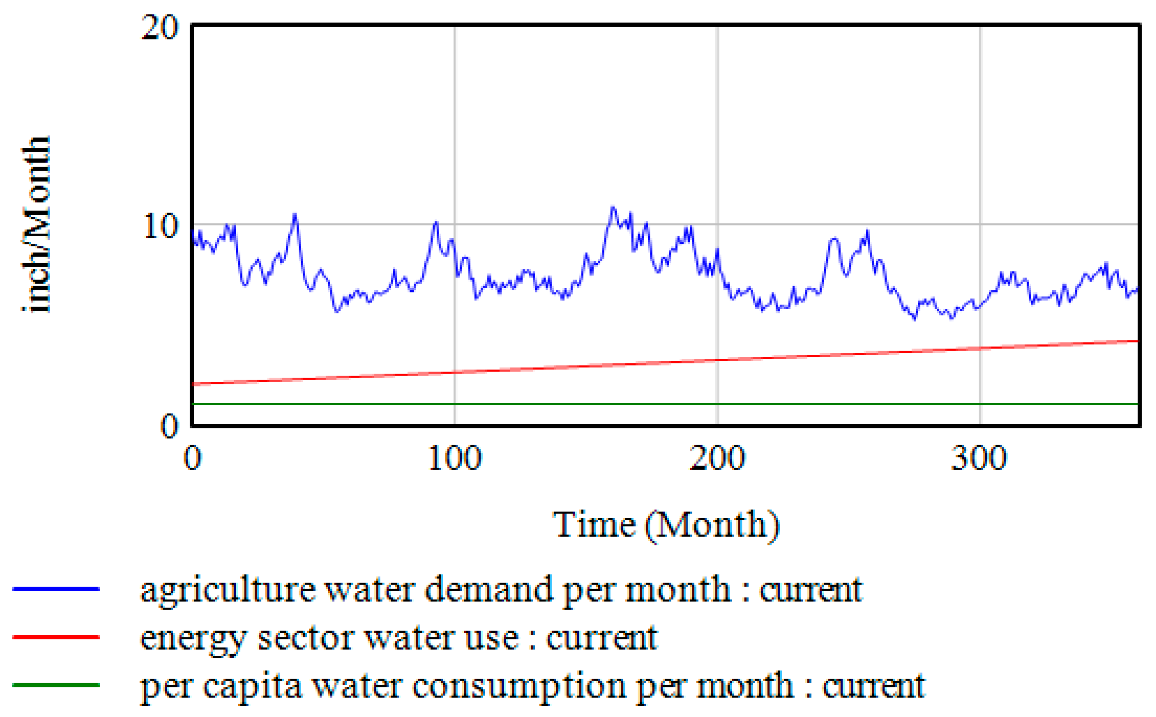
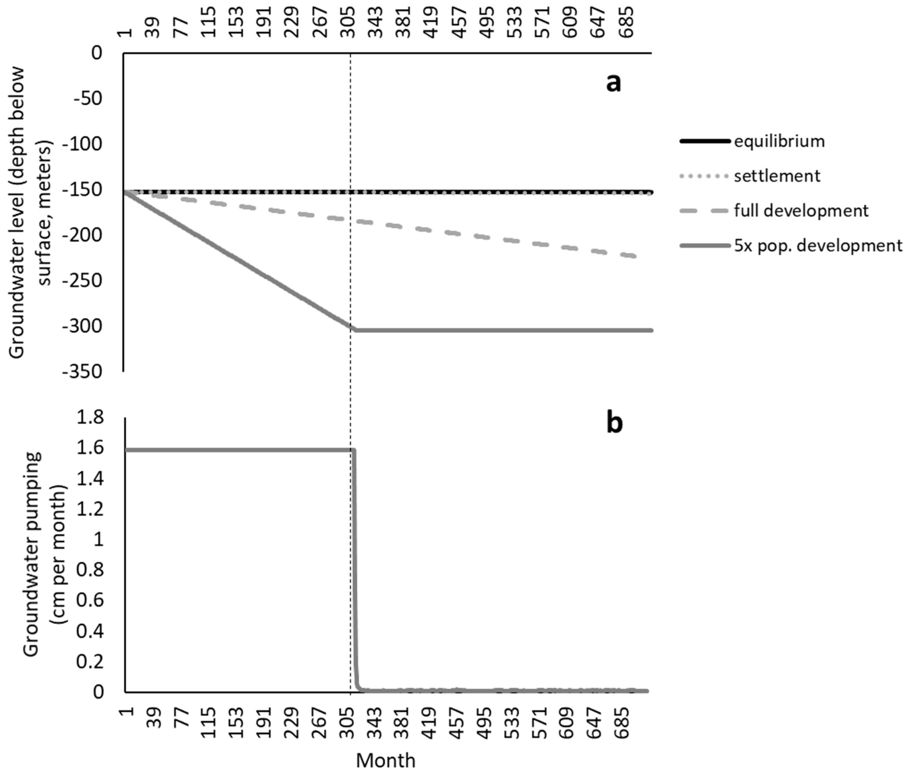
4.2. Model Assessment

Before simulation experiments were designed and implemented, the model was tested by parameterizing the initial model in equilibrium [6,64]. The equilibrium model was tested for four alternative extreme conditions:

• Average recharge (inflow) with no pumping (outflow).
• No recharge (inflow) with pumping (outflow) given surface development in a settlement phase (5% land in agriculture with base demand of 2.4 cm per month, consumptive human use of 1.27 cm per month and industrial use of 2.54 cm per month).
• No recharge (inflow) with pumping (outflow) given the surface completely developed (100% land in agriculture with base demand of 30.48 cm per month, consumptive human use of 6.35 cm per month and industrial use of 12.7 cm per month).
• No recharge (inflow) with pumping (outflow) given the surface fully developed (same parameter values as above) with five times the population demand on consumptive municipal use.

After initial model assessment, the model was calibrated to the generalizable observed trends and patterns over time in groundwater systems in Texas. Rather than calibrate to a single case, we calibrate the model to the general behavior mode expressed by groundwater aquifer levels observed throughout Texas (Figure 1) which allowed for keeping the model as simple as possible in terms of its feedback and auxiliary variable complexity but robust enough to express a variety of possible behaviors. Parameter estimates (in Table 2) were either gleaned or approximated from observed sources or relationships or settled upon after brief hand calibration procedure to match model behavior first to equilibrium behavior (similar to [6]) and then to the observed behavior patterns (Figure 1). To initialize the calibration or observed scenario run, we parameterized the model using 75% land in agriculture and base water demand per month of 30.48 cm, population grows 100% or up to two times the initial population level over the 30-year period (similar to observed population level), and industrial use grows in proportion to population growth. The calibration run also included feedback for cost of pumping on applied irrigation demand (B-loop “cost regulation on pumping” in Figure 3), whereby for every unit-depth reduction in groundwater level irrigation demand decreases 0.2% via additional pumping costs.

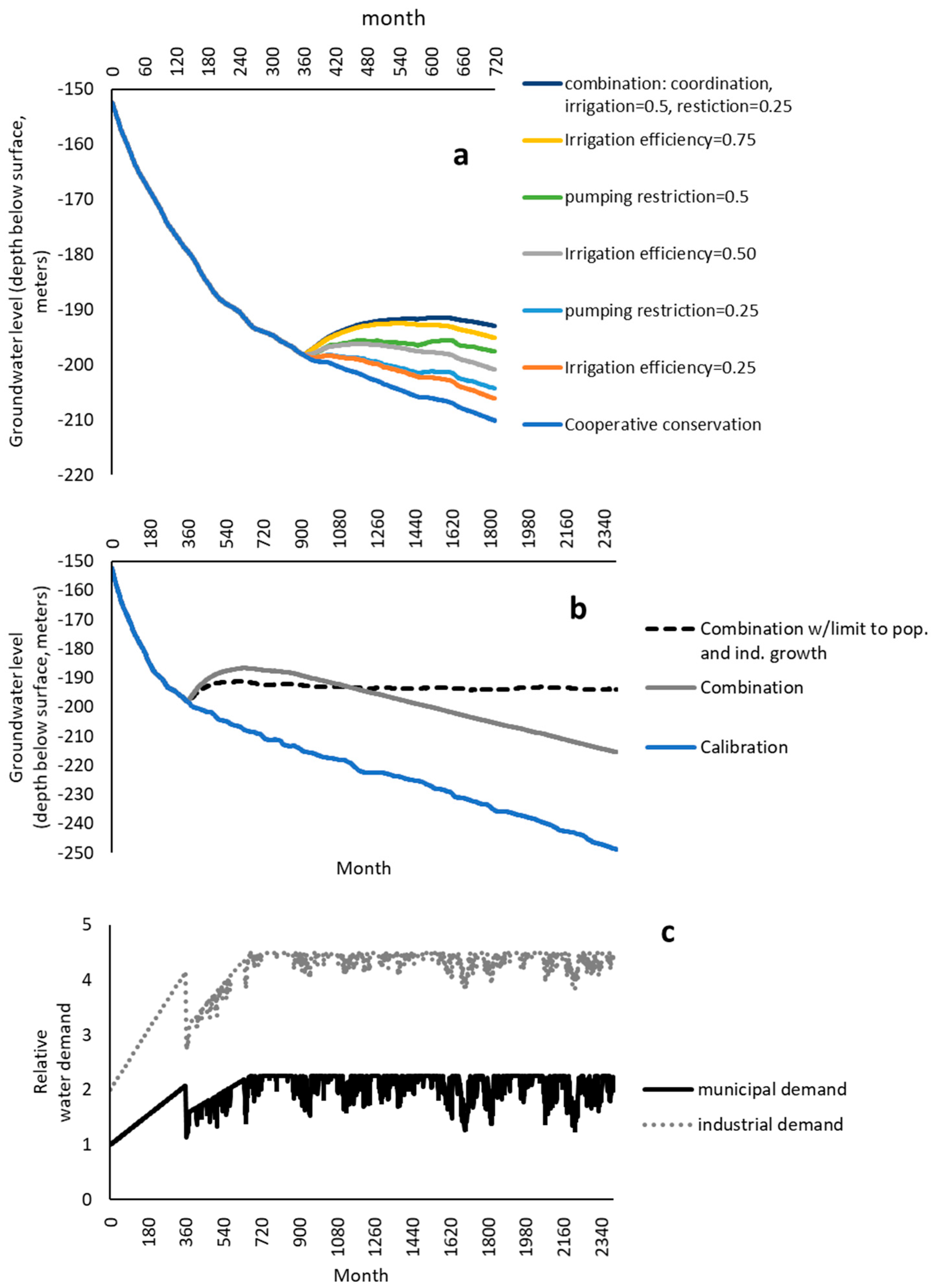
4.3. Experimental Simulation Design

The experimental simulation design followed the procedure in [64] and included a control, the base case calibration run that captured the overarching trends and patterns in groundwater levels, with treatments for the following:

• Improved irrigation efficiency (25%, 50%, 75% reduction in base irrigation demand due to improvements in irrigation efficiency).
• Policies restricting pumping rates in the municipal and industrial sectors (up to 25% reduction in the growth in pumping rates from the base case).
• Cooperative conservation (whereby base agricultural demand in permanently lowered but per capita water consumption is reduced in proportion to agricultural shortfalls during drought to maintain agricultural production). The test represented a feedback loop tradeoff which starts with agriculture base irrigation demand being dropped, but when precipitation declines and stresses agricultural systems, municipal and industrial will proactively conserve.
• A combination treatment which included cooperative conservation, 50% improvement in irrigation efficiency, and 25% pumping rate reduction in municipal and industrial sectors.

For each simulation experiment, the test began after the calibration period (month 360) for an additional 360 months (or 30 years) ending at month 720. Before running any experiments, several assumptions about future trajectories in population and industrial demand were needed. We assumed that population continues to grow at 3.6% per year. Industrial use grows in proportion to population growth with an additional growth factor of 0.006% per month to account for standard of living increases. After running the above simulations, we completed a final simulation experiment whereby we “scanned for sustainability”—searching for a parameterization scheme that could achieve a stable groundwater level into the far future (>720 months).

5. Results

5.1. Model Assessment Results

The base model behavior is shown for the four extreme condition test results (Figure 5a). The average recharge with no pumping performed as expected with a sustainable groundwater level over time. The test for settlement development (5% land in agriculture with base demand of 2.4 cm per month, consumptive human use of 1.27 cm per month and industrial use of 2.54 cm per month) also produced near-equilibrium behavior. Under full surface development (100% land in agriculture with base demand of 30.48 cm per month, consumptive human use of 6.35 cm per month and industrial use of 12.7 cm per month), groundwater levels declined at an increasing rate over time, ending with approximately half of the aquifer depleted. In the full surface development with five times the population demand, groundwater declined at an even greater rate until the aquifer was essentially depleted by month 324 after which pumping was no longer possible (Figure 5b).

Given the preliminary assessment tests showed that the physical hydrological flows of the model were operating properly, we calibrated the model to the general reference mode behavior expressed across aquifers in the Texas study area. The calibration run increased population growth (and therefore municipal and industrial use) as expected (Figure 6a) which yielded groundwater level reductions from 150 to 198 m depth below the surface (Figure 6b), an approximate 32% reduction. Behaviorally, this matched well the observed patterns of groundwater, which have declined at similar rates over similar time periods (Figure 1).

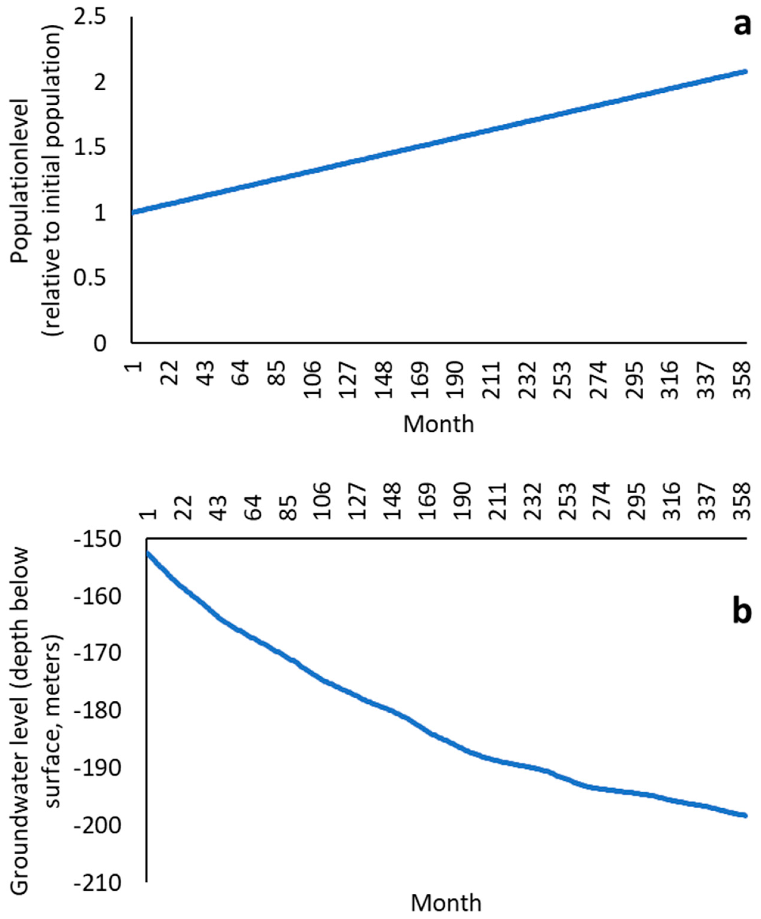
5.2. Experimental Simulation Results

Compared to the base case, all treatments produced behaviorally significant changes to groundwater levels except for cooperative conservation which did not yield a significant difference (Figure 7a). The cooperative conservation strategy failed because, although agricultural and municipal sectors are working collectively to manage the variability in water supply, no changes were made to water demand, which continued to increase with expected population and industrial growth. On the other hand, the greater the irrigation efficiency gain in agriculture or municipal and industrial pumping rate restriction (i.e., reductions in demand), the greater the impact on groundwater level recovery after month 360 (Figure 7a). The most significant treatment was the combination treatment, which included the cooperative conservation strategy, irrigation efficiency gain of 50% and municipal and industrial pumping rate restriction of 25%. Despite the improvements in groundwater levels from month 360 to month 600, after month 600 groundwater level begins declining again given the overall demand for water continues to increase given population and industrial growth. In the long-term (>720 months), this scenario did outperform the calibrated base case by 13–14%, but still yielded declining groundwater levels (Figure 7b).

In order to identify possible parameterization schemes that could achieve groundwater sustainability, we conducted a final ad hoc model treatment to alter inflow and outflow parameter values “scanning for sustainability” pathways in the far future. What we identified was that, if the combination strategy (described above) were coupled to one additional inflow strategy and one additional outflow strategy, groundwater level could sustain its partial recovery into the long-term. The inflow strategy included strategic land conservation for improved recharge zone potential (increasing recharge rate from 3.7% to 7.4%) and limiting municipal and industrial demand growth to no more than two times the initial population level, at which point no new demand growth was allowed Only by limiting population and industrial growth after month 360 to double the initial values (Figure 7c) were the extensive cooperation (seasonal shifting of demand in response to agricultural needs arising from drought—i.e., when drought is significant enough, municipal and industry users decrease their demand to support agriculture before returning to normal demand during non-drought periods) and conservation efforts, namely irrigation efficiency and pumping restrictions, were groundwater levels able to achieve some level of sustainability (dashed line in Figure 7b).

5.3. Systems Thinking as a Methodology to Explore the Groundwater–Ecosystem Service Nexus

Applying the systems thinking perspective to the simulation results provides a useful lens through which to explore the groundwater resources–ecosystem services nexus. Groundwater pumping represents fulfillment of economic demand for provisioning ecosystem services. As shown in both the case study and simulated data, short-term pumping to meet immediate needs erodes long-term security of groundwater aquifer capacity to fulfill a full range of ecosystem services related to groundwater (described in Section 2 above, Ecosystem services of groundwater aquifer systems). The critical trade-off being made then pertains to the imbalance in prioritization of short-term and long-term groundwater services utilization. Despite the feedback accounting for increasing pumping costs and the adaptive modification or irrigation demand based on precipitation trends, groundwater withdrawals continued to exceed the expected recharge rate. Only when economic drivers (industrial, municipal, and urban demand) and changes in population were stabilized and no longer growing did long-term groundwater recharge and withdrawals equilibrate and were therefore capable of maintaining (at least in part) supporting and regulating services influenced by groundwater. The stock-flow feature of groundwater systems requires that in order to sustain groundwater levels and their associated ecosystem services, outflows via pumping must be reduced. At this time, short-term economic incentives, structures (e.g., fragmented water rights) and feedbacks have not reached the point needed to induce compensating feedback mechanisms in the form of conservation mandates or use restrictions, such as in other common good resource situations, needed to curb exploitative pumping rates back in line with recharge rates.

Socially, an important discussion point among water stakeholders is the need for greater cooperation among different classes of water users to address contemporary issues. Our model reflected the siloed nature of water rights among users, with independent variables for either agricultural use, industrial use, and municipal and urban use. The simulation experiment to link users through strategic cooperation had only marginal impact on groundwater because total demand did not change, it only shifted relative demand among varying users at any point in time.

More technical scenarios included altering the demand parameters among water users via either irrigation efficiency (in the agricultural sector) or pumping restrictions (in the industrial, municipal, and urban sectors). Irrigation efficiency in attempt to use the same or less volume of water to more (i.e., improve the “crop per drop”) rewards innovation to reduce direct use of irrigation applications as well as minimize conveyance losses to the environment. The advantages of such an approach from an ecosystem service viewpoint is that any gains in irrigation efficiency, ceteris parabus, will extend the useful life of provisioning service capacity of the resource. Because the behavior changes by irrigators required to achieve this outcome is incentivized by public policies (from local to federal levels) and comes with financial incentives (e.g., reduced variable expenses, improved revenues, or both), investment in irrigation efficiency measures continues to be an attractive groundwater conservation strategy. The trade-off is that supporting and regulating services may continue to degrade via weakening the links in shallow groundwater recharge or surface water–groundwater connectivity, which is often supported by irrigation which replenishes surface layer moisture, or elimination of non-consumptive uses of groundwater at the surface, such as refilling on-farm irrigation reservoirs which provide a habitat source and connectivity for biodiversity while in short-term storage prior to use.

Similarly, pumping restrictions, such as conservation mandates imposed by municipalities to curb consumptive water use in periods of stress, possess a similar set of trade-offs. Like irrigation efficiency measures, pumping restrictions extend the useful life of provisioning service capacity. However, pumping restrictions can also significantly enhance supporting and regulating services since any uses of water must be reasonable from an environmental or health standpoint (e.g., cities prioritizing reduced water use via higher costs or penalties for aesthetic or recreation values like lawns or turfgrass monocultures and rewarding creative approaches of efficient water use such as xeriscaping or urban or community supported agricultural uses). The drawback to using restrictions on pumping are that the behavioral changes needed to sustain change are costly psychologically (incentives are legal and regulatory rather than economic in nature which can be immediately perceived at “targeting” certain users over others) and financially (through potential loss of provisioning services but also opportunity costs in cultural ecosystem services such as aesthetic values of real estate, recreation and outdoor sports and activities, etc.). The concern is that any water used today to support cultural and economic traditions, although may deplete groundwater faster, is more socially preferable compared to stringent conservation of resources, which slows extraction but potentially dislodges socio-cultural connections and benefits.

Finally, in the scenario named “scanning for sustainability”, we adaptively updated particular parameters or functions in the combination simulation experiment until the recharge rate (inflow) and pumping rate (outflow) were equal and therefore the groundwater stock would cease decline and remain in equilibrium. Achieving long-term groundwater sustainability in this fashion is based on several core principles of system dynamics: stocks can only change via inflows and outflows, and the difference between inflow and outflow rates (also called the net flow or rate) determines the trajectory of change in a stock. Given observations and evidence (Section 3.1 and Section 3.2 above, Figure 1 and Figure 2) it is widely accepted that pumping withdrawals (outflows) exceed recharge (inflows). The “scanning for sustainability” scenario revealed that the highest leverage in reversing the decline in groundwater level came from a combination of outflow-based strategies (irrigation efficiency, pumping restriction, and cooperation among users) and inflow-based strategies (land conservation and management for improved recharge potential) under a broader population and socio-economic context which is no longer growing. In other words, the longer population and economic growth continues, the longer it will take to balance inflow and outflow rates (and therefore ecosystem service capacity) even if all irrigation, industrial, and municipal users adopt best-management practices to increase efficiency, reduce losses, and curb consumption.

5.4. Limitations and Future Work

Although the model provided a simplified yet dynamic laboratory for examining groundwater dynamics, there were a number of caveats or weaknesses to the approach. First, the model was highly aggregated. The low resolution thus does not capture the complexities of substrate hydrology and geology, layered aquifer networks, surface water–groundwater connectivity relationships, differentiated recharge zones, diversified land management, or interactions of any of the above. In addition, there was no connection between population, land use, and recharge rate, which itself is influenced by land surface conditions and thereby indirectly through population. Expanding the model to better capture some of these structures and relationships in as simple means possible remains an area of future modeling work capable to experimenting with a broader suite of intervention strategies (e.g., artificial recharge which couples inflow back to groundwater with pumping and surface use).

6. Conclusions

Groundwater provides a critical link in the maintenance of a wide variety of ecosystem services, yet its role and importance has not received the same attention and conservation investment relative to other ecosystem service perspectives. The systems thinking approach used here provided a comprehensive methodology to understand complex and interdependent groundwater issues, particularly as they impact Texas, USA, but such interdependent dynamics will be relevant in other groundwater systems globally given commonly shared threats and drivers: growth in population, urbanization, and agriculture and declining recharge rates. Beginning with events, trends, and underlying structure and mental models (which helped to visualize the relationships between people and assumptions in the system), we crafted a causal loop diagram to better appreciate the types of feedback processes involved in the issue and the various perspectives of stakeholders involved. Those insights informed and provided real-world context for the system dynamics model. The calibration model run revealed a 32% reduction in groundwater levels with increasing population growth, while the combination treatment showed potential for partial groundwater recovery in the moderate- to long-term. The combination treatment, including cooperative conservation, irrigations efficiency gain and pumping rate restriction, had the most significant impact on groundwater level recovery. Such an approach however will require an increase in science-based education and extension programming that focus on irrigation and best management practices to adopt water conservation practices for all users. If not, our model projections point to continued decline and deterioration of groundwater resources which will require more severe interventions to reverse and stabilize groundwater declines the longer time passes before implementation. Future modeling work should focus on expanding the model for more groundwater sustainability assessments. Expanding the model to better capture structures and relationships between geology, surface–groundwater connectivity, substrate hydrology, land use, recharge rate and population remains an area of future work.

References

1. Serrano, S.E. Hydrology for Engineers, Geologists, and Environmental Professionals; HydroScience: Lexington, KY, USA, 2010. [Google Scholar]
2. Griebler, C.; Avramov, M.; Hose, G. Groundwater ecosystems and their services: Current status and potential risks. In Atlas of Ecosystems Services: Drivers, Risks, and Societal Responses; Springer: Berlin/Heidelberg, Germany, 2019; pp. 197–203. [Google Scholar]
3. Vollmer, D.; Kremena, B.; Esmail, B.A.; Guerrero, P.; Nagabhatla, N. Incorporating ecosystem services into water resources management—Tools, policies, promising pathways. Environ. Manag. 2022, 69, 627–635. [Google Scholar] [CrossRef] [PubMed]
4. Russo, T.A.; Lall, U. Depletion and response of deep groundwater to climate-induced pumping variability. Nat. Geosci. 2017, 10, 105–108. [Google Scholar] [CrossRef]
5. Turner, B.L.; Menendez, H.M., III; Gates, R.; Tedeschi, L.O.; Atzori, A.S. System dynamics modeling for agricultural and natural resource management issues: Review of some past cases and forecasting future roles. Resources 2016, 5, 40. [Google Scholar] [CrossRef]
6. Ford, A. Modeling the Environment; Island Press: Washington, DC, USA, 2010. [Google Scholar]
7. Reid, W.V.; Mooney, H.A.; Cropper, A.; Capistrano, D.; Carpenter, S.R.; Chopra, K.; Dasgupta, P.; Dietz, T.; Duraiappah, A.K.; Hassan, R.; et al. Millennium Ecosystem Assessment. Ecosystems and Human Well-Being: Synthesis; Island Press: Washington, DC, USA, 2005. [Google Scholar]
8. Mpanga, I.K.; Idowu, O.J. A decade of irrigation water use trends in Southwestern USA: The role of irrigation technology, best management practices, and outreach education programs. Agric. Water Manag. 2021, 243, 106438. [Google Scholar] [CrossRef]
9. Döll, P.; Fiedler, K. Global-scale modeling of groundwater recharge. Hydrol. Earth Syst. Sci. 2008, 12, 863–885. [Google Scholar] [CrossRef]
10. Siebert, S.; Burke, J.; Faures, J.M.; Frenken, K.; Hoogeveen, J.; Döll, P.; Portmann, F.T. Groundwater use for irrigation—A global inventory. Hydrol. Earth Syst. Sci. 2010, 14, 1863–1880. [Google Scholar] [CrossRef]
11. Grafton, R.Q.; Williams, J.; Perry, C.J.; Molle, F.; Ringler, C.; Steduto, P.; Udall, B.; Wheeler, S.A.; Wang, Y.; Garrick, D.; et al. The paradox of irrigation efficiency. Science 2018, 361, 748–750. [Google Scholar] [CrossRef]
12. Lezzaik, K.; Milewski, A.; Mullen, J. The groundwater risk index: Development and application in the Middle East and North Africa region. Sci. Total Environ. 2018, 628–629, 1149–1164. [Google Scholar] [CrossRef]
13. Asadi, A.; Barati, A.A.; Kalantari, K. Analyzing and modeling the impacts of agricultural land conversion in Iraan. Bus. Manag. Rev. 2014, 4, 110–118. [Google Scholar]
14. Steward, D.R.; Bruss, P.J.; Yang, X.; Staggenborg, S.A.; Welch, S.M.; Apley, M.D. Tapping Unsustainable Groundwater Stores for Agricultural Production in the High Plains Aquifer of Kansas, projections to 2110. Proc. Natl Acad. Sci. USA 2013, 10, E3477–E3486. [Google Scholar] [CrossRef]
15. Partridge, T.; Winter, J.; Kendall, A.; Basso, B.; Pei, L.; Hyndman, D. Irrigation benefits outweigh costs in more US croplands by mid-century. Commun. Earth Environ. 2023, 4, 274. [Google Scholar] [CrossRef]
16. Colaizzi, P.D.; Gowda, P.H.; Marek, T.H.; Porter, D.O. Irrigation in the Texas High Plains: A brief history and potential reductions in demand. J. Int. Comm. Irrig. Drain. 2009, 58, 257–274. [Google Scholar] [CrossRef]
17. Lauer, S.; Sanderson, M.R.; Manning, D.T.; Suter, J.F.; Hrozencik, R.A.; Guerrero, B.; Golden, B. Values and groundwater management in the Ogallala Aquifer region. J. Soil Water Conserv. 2018, 73, 593–600. [Google Scholar] [CrossRef]
18. Griebler, C.; Brielmann, H.; Haberer, C.M.; Kaschuba, S.; Kellermann, C.; Stumpp, C.; Hegler, F.; Kuntz, D.; Hertkorn, S.W.; Lueders, T. Potential impacts of geothermal energy use and storage of heat on groundwater quality, biodiversity, and ecosystem processes. Environ. Earth Sci. 2016, 75, 1391. [Google Scholar] [CrossRef]
19. Tissen, C.; Benz, S.A.; Menberg, K.; Bayer, P.; Blum, P. Groundwater temperature anomalies in central Europe. Environ. Res. Lett. 2019, 14, 104012. [Google Scholar]
20. Gleeson, T.; Wada, Y.; Bierkens, M.F.P.; Van Beek, L.P.H. Water balance of global aquifers revealed by groundwater footprint. Nature 2012, 488, 197–200. [Google Scholar] [CrossRef] [PubMed]
21. Gleeson, T.; Befus, K.M.; Jasechko, S.; Luijendijk, E.; Cardenas, M.B. The global volume and distribution of modern groundwater. Nat. Geosci. 2015, 9, 161–167. [Google Scholar]
22. Vigerstol, K.L.; Aukema, J.E. A comparison of tools for modeling freshwater ecosystem services. J. Environ. Manag. 2011, 92, 2403–2409. [Google Scholar]
23. FAO. Shared Global Vision for Groundwater Governance 2030 and a Call-for-Action; Groundwater Governance: A Global Framework for Action; FAO: Rome, Italy, 2015. [Google Scholar]
24. Qiu, J.; Wardropper, C.B.; Rissman, A.R.; Turner, M.G. Spatial fit between water quality policies and hydrologic ecosystem services in an urbanizing agricultural landscape. Landsc. Ecol. 2017, 32, 59–75. [Google Scholar] [CrossRef]
25. Larned, S.T. Phreatic groundwater ecosystems: Research frontiers for freshwater ecology. Freshw. Biol. 2012, 57, 885–906. [Google Scholar] [CrossRef]
26. Hutchins, B.T. The Conservation Status of Texas groundwater invertebrates. Biodivers. Conserv. 2017, 27, 475–501. [Google Scholar] [CrossRef]
27. Cook, B.R.; Spray, C.J. Ecosystem services and integrated water resource management: Different paths to the same end? J. Environ. Manag. 2012, 109, 93–100. [Google Scholar] [CrossRef]
28. Herrera-Franco, G.; Montalván-Burbano, N.; Carrion-Mero, P.; Bravo-Montero, L. Worldwide research on socio-hydrology: A bibliometric analysis. Water 2021, 13, 1283. [Google Scholar] [CrossRef]
29. Gu, J.; Sun, S.; Wang, Y.; Li, X.; Sun, J.; Qi, X. Sociohydrology: An effective way to reveal the coupled evolution of human and water Systems. Water Resour. Manag. 2021, 35, 4995–5010. [Google Scholar] [CrossRef]
30. Breyer, B.; Zipper, S.C.; Qui, J. Sociohydrological impacts of water conservation under anthropogenic drought in Austin, TX (USA). Water Resour. Res. 2018, 54, 3062–3080. [Google Scholar] [CrossRef]
31. Gunda, T.; Turner, B.L.; Tidwell, V.C. The influential role of sociocultural feedbacks on community-managed irrigation system behaviors during times of water stress. Water Resour. Res. 2018, 54, 2697–2714. [Google Scholar] [CrossRef]
32. Turner, B.L.; Tidwell, V.; Fernald, A.; Rivera, J.A.; Rodriguez, S.; Guldan, S.; Ochoa, C.; Hurd, B.; Boykin, K.; Cibils, A. Modeling acequia irrigation systems using system dynamics: Model development, evaluation, and sensitivity analyses to investigate effects of socio-economic and biophysical feedbacks. Sustainability 2016, 8, 1019. [Google Scholar] [CrossRef]
33. Turner, B.L.; Tidwell, V.C.; Fernald, A.; Rivera, J.A.; Rodriguez, S.; Gulden, S.; Ochoa, C.; Hurd, B.; Boykin, K.; Cibils, A. Connection and Integration: A Systems Approach to Exploring Acequia Community Resiliency. In Southwestern United States: Elements of Resilience; New Mexico State University: Las Cruces, NM, USA, 2021; p. 58. [Google Scholar]
34. Stroh, D.P. Systems Thinking for Social Change: A Practical Guide to Solving Complex Problems, Avoiding Unintended Consequences, and Achieving Lasting Results; Chelsea Green Publishing: Chelsea, VT, USA, 2015. [Google Scholar]
35. Ford, D.N. A system dynamics glossary. Syst. Dyn. Rev. 2019, 35, 369–379. [Google Scholar] [CrossRef]
36. Texas Almanac Aquifers of Texas. Available online: https://www.texasalmanac.com/articles/aquifers-of-texas (accessed on 5 December 2022).
37. Texas Water Development Board. Aquifers of Texas, Report 380. Available online: https://www.twdb.texas.gov/groundwater/aquifer/index.asp (accessed on 8 December 2024).
38. Environment Defense Fund. Available online: https://edf.org/media/texas-groundwater-supplies-are-danger-reports-say (accessed on 5 December 2022).
39. Texas Tribune. Available online: https://www.texastribune.org/2013/05/07/texas-groundwater-dropped-sharply-amid-droughtstud/ (accessed on 5 December 2022).
40. Holzer, T.L. Preconsolidation stress of aquifer systems in areas of induced land subsidence. Water Resour. Res. 1981, 17, 693–703. [Google Scholar] [CrossRef]
41. Baddour, D.; New Study Shows Rate of Groundwater Decline Slowing in Texas. Energy and Environment Reporting for Texas. National Public Radio 2014 (July 17). Available online: https://stateimpact.npr.org/texas/2014/07/17/new-study-shows-rate-of-groundwater-decline-slowing-in-texas/ (accessed on 5 December 2022).
42. Federal Reserve Bank of Dallas. Available online: https://dallasfed.org/research/swe/2020/swe20001 (accessed on 5 December 2022).
43. Rosepiler, M.J.; Reilinger, R. Land subsidence due to water withdrawal in the vicinity of Pecos, Texas. Eng. Geol. 1977, 11, 295–304. [Google Scholar] [CrossRef]
44. Chauduri, S.; Ale, S. Long-term (1930–2010) trends in groundwater levels in Texas: Influences of soils, land cover and water use. Sci. Total Environ. 2014, 490, 379–390. [Google Scholar] [CrossRef] [PubMed]
45. Texas Water Development Board. Available online: https://www.waterdatafortexas.org/groundwater (accessed on 8 December 2024).
46. NOAA National Centers for Environmental Information. Available online: https://www.ncei.noaa.gov/access/monitoring/climate-at-a-glance/statewide/time-series (accessed on 4 June 2024).
47. United States Census Bureau. Available online: https://www.census.gov/data/tables-series/dec/popchange-data-text.html (accessed on 1 May 2021).
48. USDA National Agricultural Statistics Service. Available online: https://quickstats.nass.usda.gov/ (accessed on 8 December 2024).
49. Flores-Lopez, C.; Turner, B.L.; Hanagriff, R.; Bhandari, A.; Sinha, T. South Texas Water Resource Mental Models: A Systems Thinking, Multi-stakeholder Case Study. J. Contemp. Water Res. Educ. 2022, 176, 15–35. [Google Scholar] [CrossRef]
50. De Brito Neto, R.; Santos, C.A.G.; Mulligan, K.; Barbato, L. Spatial and temporal water-level variations in the Texas portion of the Ogallala Aquifer. Nat. Hazards 2016, 80, 351–365. [Google Scholar] [CrossRef]
51. Runkle, J.; Kunkel, K.E.; Nielson-Gammon, J.; Frankson, R.; Champion, S.M.; Stewart, B.C.; Romolo, L.; Sweet, W. Texas State Climate Summary; NOAA Technical Report NESDIS 150-TX: Silver Spring, MD, USA, 2022; p. 5. [Google Scholar]
52. United States Department of Agriculturee. Available online: https://www.nass.usda.gov/Publications/AgCensus/2012/Online_Resources/Farm_and_Ranch_Irrigation_Survey/ (accessed on 20 October 2019).
53. U.S. Department of Agriculture, Economic Research Service. Available online: https://www.ers.usda.gov/topics/farm-economy/farm-sector-income-finances/ (accessed on 7 February 2024).
54. Haacker, E.M.K.; Catterman, K.A.; Smidt, S.J.; Kendall, A.D.; Hyndman, D.W. Effects of Management areas, drought, and commodity prices on groundwater decline patterns across the High Plains Aquifer. Agric. Water Manag. 2019, 218, 259–273. [Google Scholar] [CrossRef]
55. Watershed Association. Available online: https://wimberlywatershed.org (accessed on 5 December 2022).
56. Sustainable Statewide Water Resources Management in Texas. Available online: https://wrap.engr.tamu.edu (accessed on 5 December 2022).
57. Forrester, J.W. Principles of Systems; Wright Allen Press: Cambridge, MA, USA, 1971. [Google Scholar]
58. Sterman, J. Business Dynamics, Systems Thinking and Modeling for a Complex World; Irwin/McGraw-Hill: Chicago, IL, USA, 2000. [Google Scholar]
59. Eberlein, R.L.; Peterson, D.W. Understanding models with Vensim™. Eur. J. Oper. Res. 1992, 59, 216–219. [Google Scholar] [CrossRef]
60. Barati, A.A.; Azadi, H.; Scheffran, J. A system dynamics model of smart groundwater governance. Agric. Water Manag. 2019, 20, 502–518. [Google Scholar] [CrossRef]
61. Giordano, R.; Brugnach, M.; Vurro, M. System Dynamic Modelling for Conflicts Analysis in Groundwater Management. In Proceedings of the International Congress on Environmental Modelling and Software, Leipzig, Germany, 1 July 2012; p. 105. [Google Scholar]
62. Turner, B.L.; Kodali, S. Soil system dynamics for learning about complex, feedback-driven agricultural resource problems: Model development, evaluation, and sensitivity analysis of biophysical feedbacks. Ecol. Model. 2020, 428, 109050. [Google Scholar] [CrossRef]
63. Laio, F.; Porporato, A.; Laio, F.; Ridolfi, L. Plants in water-controlled ecosystems: Active role in hydrologic processes and response to water stress: II. Probabilistic soil moisture dynamics. Adv. Water Resour. 2001, 24, 707–723. [Google Scholar] [CrossRef]
64. Turner, B.L. Model laboratories: A quick-start quide for design of simulation experiments for dynamic systems models. Ecol. Model. 2020, 434, 109246. [Google Scholar] [CrossRef]
Figure 1. Trends over time in varying groundwater aquifer depths in Texas: Carrizo−Wilcox (panels a,b); Trinity (panels c,d); and Ogallala (panels e,f); all data are available from the Texas Water Development Board [45].
Systems 12 00583 g001
Figure 2. Other trends and patterns over time relevant for Texas groundwater systems: Texas population from the U.S. Census Bureau (panel a); observed statewide precipitation mean and anomaly (panel b; [46]); production of two commonly irrigated crops, cotton and peanuts (panels c,d; [48]); irrigated area (panel e; [52]); and mean dollar per acre revenue (rev), expenses (exp), and profit of U.S. farms (panel f; [53]).
Systems 12 00583 g002
Figure 3. Feedback processes which drive continual groundwater reduction over time: Links denoted ‘S’ represent the same relationship whereby variables at the arrowhead move the same direction as their causal predecessor at the arrow tail, while links denoted ‘O’ represent an opposite causal relationship across the causal link (blue arrows). For example, as demand for water increases (decreases), pumping increases (decreases), leading to community use increasing (or decreasing) which lead to further increases (decreases) in community attractiveness and population and therefore demand for water (a reinforcing feedback process denoted R). Economic or biophysical limits to this reinforcing loop arise through the influence of groundwater volume, level, and pumping on socio-economic and hydrologic functions. For example, increased pumping costs (as a result of greater pumping), leads to financial pressure to reduce pumping rate (denoted an ‘O’ link). Likewise, groundwater volume declines, municipal costs increase (O link) after some time delay (denoted by the delay ≠ link), leading to more conservation mandates (S link) aimed at reducing demand for water (O link) and therefore pumping (a form of balancing feedback denoted B, which acts to balance or offset the growth processes).
Systems 12 00583 g003
Figure 4. System dynamics stock-and-flow diagram of the simplified groundwater model: groundwater level (stock) is influenced by inflows (recharge rate) and outflows (groundwater pumping), connected via causal feedback links (blue arrows). Experimental variables used during simulation experiments are enclosed in the boxes adjacent to the diagram.
Systems 12 00583 g004
Figure 5. Results of preliminary model assessment tests for equilibrium groundwater conditions, groundwater conditions under settlement rate of surface development (5% land in agriculture with base demand of 2.4 cm per month, consumptive human use of 1.27 cm per month and industrial use of 2.54 cm per month), groundwater conditions with full surface development (100% land in agriculture with base demand of 30.48 cm per month, consumptive human use of 6.35 cm per month and industrial use of 12.7 cm per month), and full surface development with five times the population level (panel a); when groundwater is fully depleted (i.e., no water remaining or water is simply unreachable) then feedback exists to stop groundwater pumping, a biophysical conservation check in the model (panel b).
Systems 12 00583 g005
Figure 6. Results of the calibration model run given an increase in population over time similar to the observed population growth (panel a) and the resulting groundwater level (panel b).
Systems 12 00583 g006
Figure 7. Experimental simulation results over a 30-year scenario horizon for varying rates of cooperative conservation, pumping restrictions, irrigation efficiency gains, or the combination scenario of including cooperative conservation, pumping restrictions, and efficiency gains (panel a); a far future (≈150 yr) comparison of the base case calibration, the combination scenario of cooperative conservation, pumping restrictions, and irrigation efficiency gains but with no limit to population and industrial growth, and the combination scenario under limits to population and industrial growth after 30 years (panel b); relative water demand (1 = municipal and industrial demand in 1990) in the far-future scenario under limits to growth (panel c).
Systems 12 00583 g007