Modeling and Solving the Multi-Objective Vehicle Routing Problem with Soft and Fuzzy Time Windows

Abstract

In the distribution field, distribution costs and customer service satisfaction are extremely important issues for enterprises. However, both the Vehicle Routing Problem with Soft Time Windows (VRPSTW) and the Vehicle Routing Problem with Fuzzy Time Windows (VRPFTW) have certain deficiencies in describing real-world scenarios. Therefore, this paper considers both soft time windows and fuzzy time windows, improving upon the traditional VRPSTW and VRPFTW models to establish a more comprehensive and realistic model called the Vehicle Routing Problem with Soft Time Windows and Fuzzy Time Windows (VRPSFTW). Secondly, to solve the relevant problems, this paper proposes a Directed Mutation Genetic Algorithm integrated with Large Neighborhood Search (LDGA), which fully utilizes the advantages of the Genetic Algorithm (GA) in the early stages and appropriately adopts removal and re-insertion operators from the Large Neighborhood Search (LNS). This approach not only makes efficient use of computational resources but also compensates for the weaknesses of crossover and mutation operators in the later stages of the genetic algorithm. Thereby, it improves the overall efficiency and accuracy of the algorithm and achieves better solution results. In addition, in order to solve multi-objective problems, this paper employs a two-stage solution approach and designs two sets of algorithms based on the principles of “cost priority” and “service-level priority”. Simulation experiments demonstrated that the algorithms designed in this study achieved a more competitive solving performance.

1. Introduction

The logistics industry is a fundamental, strategic, and leading sector that supports the development of the national economy. Reducing logistics costs and increasing efficiency are not only essential for the nation, society, and industry, but also for the enterprises themselves. For many companies, transportation costs are usually the largest portion of their logistics expenses. According to statistics from the National Development and Reform Commission, China’s total social logistics cost in 2023 reached CNY 18.2 trillion, a year-on-year increase of 2.3%, with the transportation cost amounting to CNY 9.8 trillion, increasing by 2.8%. The transportation cost still accounts for the largest share of the total social logistics cost and is one of the key expenditures for logistics companies. The high proportion of the transportation cost is largely influenced by the delivery costs of logistics companies. According to the “2021 Logistics Business Environment Survey” published by the China Federation of Logistics and Purchasing, delivery costs ranked fourth among the top nine items for which the surveyed companies reported the most significant cost increases, accounting for 35.5%. The persistently high delivery costs are closely related to the failure of many logistics companies to develop scientific, reasonable, and efficient delivery routes, which remains a pressing issue for many enterprises. Currently, the majority of delivery problems faced by enterprises can be categorized as the Vehicle Routing Problem (VRP) and its variants, for which further in-depth research is necessary.

The VRP was first introduced by Dantzig and Ramser in 1959, and was initially termed “The truck dispatching problem” [1]. The authors extended the concept of the Traveling Salesman Problem (TSP) by introducing the constraint of multiple vehicles. Subsequently, researchers have proposed various variants of the VRP based on different scenarios encountered in reality. These include the Capacitated Vehicle Routing Problem (CVRP) [2], Dynamic Vehicle Routing Problem (DVRP) [3], Vehicle Routing Problem with Pickup and Delivery (VRPPD) [4], the Heterogeneous Fleet VRP (HFVRP) [5], among others. The Vehicle Routing Problem with Time Windows (VRPTW) [6] is a significant variant of the VRP that is characterized by time window constraints. As a significant branch of combinatorial optimization problems, the VRPTW has attracted extensive research interest over the years.

The Vehicle Routing Problem with Soft Time Windows (VRPSTW) is an extension of the VRPTW that allows for more flexible scheduling under time window constraints. Soft time windows mean that customers can accept service outside of their specified time windows, but usually at the cost of a penalty fee. Each customer has a desired service time window, and if the vehicle arrives within this window, the service can begin normally without incurring additional costs. However, if the vehicle services the customer outside of their time window, a penalty cost is incurred. Because exceeding the time window incurs extra costs, scheduling strategies must balance timely service and cost reduction. Soft time windows provide greater scheduling flexibility compared to hard time windows, allowing vehicles to adjust their arrival and service times within certain limits to optimize the overall routes and costs. Zhang et al. [7] noted that the feasible solution space for the VRPSTW is larger than that for the VRPHTW, providing decision-makers with more options. The VRPSTW effectively simulates many scenarios wherein the time window constraints are not strict. This model makes it suitable for situations requiring flexible scheduling, such as express delivery and maintenance services, for which customers may tolerate a certain degree of early or late service. Considering both customer experience and economic benefits, soft time windows are more applicable to real-world situations. Chiang et al. [8] argue that the VRPSTW can effectively reduce delivery costs without significantly lowering customer satisfaction.

The Vehicle Routing Problem with Fuzzy Time Windows (VRPFTW) is an extended version of the vehicle routing problem that aims to address the uncertainty and vagueness of time windows. In practical applications, a customer may not only have a desired time window for receiving service but may also have a tolerable time window. Incorporating fuzzy logic to consider the flexibility of time windows allows the service to be delivered earlier or later within a certain range while also considering the corresponding customer satisfaction levels, an approach that better balances customer satisfaction and operational costs. Tang et al. [9] were among the first to consider the VRPFTW. The authors used fuzzy membership functions to describe the service-level issues related to the window violations in vehicle routing problems, and thus introduced the concept of fuzzy time windows. Based on this concept, they proposed the vehicle routing problem with fuzzy time windows. The model they established is framed as a multi-objective optimization problem, with the objective functions able to minimize the total distance and maximize the overall service level.

However, both the VRPSTW and the VRPFTW have some flaws when describing real-world scenarios, as follows:

(1)

The VRPSTW model overlooks the service levels. In some cases, violating the time windows does not directly result in any penalty costs, but customer satisfaction (the service level of the delivery side) may decrease, potentially leading to long-term profit losses.

(2)

Furthermore, in the current literature, VRPSTW models are often used to calculate the penalty costs in the objective function by directly multiplying the amount of time violated by a predetermined penalty coefficient. However, this approach is not very realistic, as it ignores the size of the customer demand, which in practice, is often related to the calculation of penalty fees.

(3)

In contrast, the VRPFTW model established by Tang et al. is overly simplistic. The objective function of this model only considers the minimization of the total distance and the maximization of the overall service level, and its service-level calculation neglects the characteristics of individual customers, and thus cannot accurately reflect the true service level of the delivery side.

In light of the increasing demand in the logistics and transportation sectors, scholars have proposed various algorithms to solve the VRPTW, aiming to enhance the efficiency of vehicle transportation logistics. Initially, researchers attempted to solve the VRPTW using exact algorithms; however, because the VRPTW is an NP-hard problem, using exact algorithms to solve large-scale VRPTWs is time-consuming. As a result, over time, scholars have proposed various heuristic algorithms to tackle the VRPTW, including the Genetic Algorithm (GA) [10], Simulated Annealing (SA) [11], Memetic Algorithm (MA) [12], Ant Colony Optimization (ACO) [13], Particle Swarm Optimization (PSO) [14], Tabu Search (TS) [15], Harmony Search (HS) [16], Large Neighborhood Search (LNS) [17], Variable Neighborhood Search (VNS) [18], and other techniques.

Up to now, no heuristic or metaheuristic algorithm has been found to be superior to other algorithms in all situations, and each algorithm has its own advantages and disadvantages; therefore, researchers have attempted to combine multiple algorithms to obtain better ones. B. Yu and colleagues proposed a hybrid algorithm that combines Ant Colony Optimization (ACO) and Tabu Search (TS) [19]. YANG SHEN and colleagues proposed a hybrid swarm intelligence algorithm that combines the Ant Colony System (ACS) and Brain Storm Optimization (BSO) algorithms [20] to minimize the total distance for solving the VRPTW. Moreover, Qichao Wu and colleagues proposed using Neighborhood Comprehensive Learning Particle Swarm Optimization (N-CLPSO) [21] to solve the VRPTW. The above studies indicate that a reasonable combination of two or more methods can enhance their advantages in specific situations and compensate for their disadvantages.

The Genetic Algorithm (GA) was first proposed by John Holland in the 1970s, and was designed based on the principles of biological evolution in nature. As a heuristic optimization algorithm, the GA has been applied to the VRPTW to find optimal delivery routes. By simulating the process of biological evolution in nature, the GA can find better solutions in large search spaces and demonstrates good robustness when dealing with complex optimization problems.

The Large Neighborhood Search (LNS) algorithm is an effective tool for solving complex combinatorial optimization problems. Paul Shaw utilized constraint programming and the LNS to address the VRPTW [22], demonstrating high accuracy and a high local search capability. Grigorios and colleagues developed a Multi-objective Large Neighborhood Search (MOLNS) algorithm to solve the VRPTW [23].

The model established in this paper is a multi-objective optimization model. One of the most commonly used heuristic algorithms for solving multi-objective vehicle routing problems is the Non-dominated Sorting Genetic Algorithm (NSGA), which was proposed by Srinivas and Deb in 1995 and is based on the concept of Pareto optimality. In 2000, the authors introduced an improved version called the NSGA-II, which incorporates an elitism strategy. The NSGA-II algorithm treats all the objectives as equally important when dealing with multi-objective optimization problems, without assigning priority to any single objective, and it seeks a set of Pareto optimal solutions through non-dominated sorting and the crowding distance, ensuring that all objectives are balanced and considered throughout the solution process. This approach is suitable for scenarios in which all objectives are equally important or it is difficult to clearly define the priorities.

The research on the above-mentioned solution algorithms has several shortcomings, as follows:

(1)

The genetic algorithm has accuracy limitations when solving the VRPTW and faces challenges such as falling into local optimal solutions and a slow convergence speed in the later stages of the algorithm. In particular, the traditional genetic operators in the algorithm may become less effective as the population converges to a certain extent, rendering their performance negligible and potentially causing negative impacts by disrupting the superior individuals within the population.

(2)

The LNS has its limitations, primarily due to its high computational resource consumption, and it can be constrained by the complexity of the search space and limitations related to computational resources, especially when dealing with large-scale problems.

(3)

In scenarios in which certain objectives require higher priority, the standard NSGA-II may struggle to produce satisfactory solutions. In reality, most decision-makers face constraints due to limited resources and often establish priorities in multi-objective optimization. In such cases, optimizing the higher-priority objectives while also attempting to optimize the lower-priority objectives may yield results that are more valuable to decision-makers.

The research and contributions of this paper are as follows:

(1)

The model established in this paper is a variant of the VRPTW that simultaneously considers soft and fuzzy time windows. The variant improves upon the traditional VRPSTW and VRPFTW models, creating a more comprehensive and realistic model called the VRPSFTW model.

(2)

Considering the issues present in the related research, in this study, we address the VRPTW model by designing a Directed Mutation Genetic Algorithm (DGA) combined with a Large Neighborhood Search (LNS) algorithm (LDGA). This approach leverages the advantages of the genetic algorithm in the early stages while mitigating the slower convergence speed in the later stages, thereby improving the overall efficiency and accuracy of the algorithm, leading to better solution results.

(3)

For the multi-objective problem, this paper employs a two-stage solution approach, designing two sets of algorithms based on the principles of “cost priority” and “service-level priority”. It moves away from traditional swarm intelligence algorithms that use the optimal solution from the last generation as the final answer, instead defining a “historical optimal solution” variable that is continuously updated during iterations to seek Pareto solutions. Additionally, a population update operator is introduced to incorporate the “historical optimal solution” into the population.

(4)

The paper also optimizes the start service time by designing an operator to determine it.

(5)

The simulation results demonstrate that the proposed algorithms achieve notable solution performance.

The structure of the rest of this paper is as follows: Section 2 establishes a VRPSFTW model; Section 3 details the specific design of the LDGA and two-stage algorithm; Section 4 presents the relevant experimental results and their analysis; Section 5 concludes the paper and discusses future research directions.

2. Model Formulation

2.1. Problem Description

Currently, many delivery problems in real-world scenarios can be classified according to the VRPTW and its variants. The VRPTW is a classic, single-objective, combinatorial optimization problem, and the model established in this study is a variant of the VRPTW that simultaneously considers soft and fuzzy time windows, improving upon the traditional VRPSTW and VRPFTW models to create a model that better fits real-world scenarios.

The following assumptions are made for the model established in this study:

(1)

There is a distribution center and a set of customers;

(2)

The distribution center has a certain number of vehicles, all of which have the same loading capacity limit, driving speed, fixed costs, and unit transportation costs;

(3)

Each customer has a specific demand, location coordinates, a desired service time window, and a tolerable service time window;

(4)

The delivery vehicles depart from the distribution center, complete the delivery services in sequence, and then return to the distribution center;

(5)

The number of vehicles is sufficient to complete the delivery tasks, and the capacity of each vehicle is greater than the demand of a single customer, and the demand of a customer can be satisfied by a single vehicle;

(6)

Each customer must be served by exactly one vehicle according to a single delivery route plan;

(7)

If a vehicle arrives at customer i before their tolerable service time window, then it must wait, incurring waiting costs;

(8)

If the service time for customer i falls outside their desired service time window, then a penalty is applied;

(9)

The relationship between the time at which a vehicle starts serving customer i and the tolerable service time window, along with the demand of customer i, determine the service level provided to customer i.

The optimization objective of the problem is to determine the routes for each vehicle to meet the customer demand while minimizing the overall delivery cost and maximizing the overall service level.

2.2. Notations

2.2.1. Sets and Parameters

$N$: Number of customers;

$K$: Maximum number of vehicles;

$m$: Set of vehicle indexes, m = {1, 2, 3, …, K};

$n$: Set of customer indexes, n = {1, 2, 3, …, N}; index 0 represents the distribution center;

$h, i, j$: Node indices, where $h, i, j\in \{\mathrm{0,1},\mathrm{2,3},\dots ,N\}$;

$k$: Vehicles indices, where $k\in m$;

$d_{ij}$: Distance from customer i to customer j;

$d_{0i}$: Distance from the distribution center to customer i;

$q_i$: Demand of customer i;

$a_i$: Start time of the time window during which customer i wishes to receive service;

$b_i$: End time of the time window during which customer i wishes to receive service;

$A_i$: Start time of the time window in which customer i can tolerate receiving service;

$B_i$: End time of the time window in which customer i can tolerate receiving service;

$s_i$: Service time for customer i;

$a_0$: Start time of the time window for the distribution center;

$b_0$: End time of the time window for the distribution center;

$P_1$: Penalty coefficient for violating time window constraint 1;

$P_2$: Penalty coefficient for violating time window constraint 2;

$P_3$: Penalty coefficient for violating time window constraint 3;

$Q$: Maximum load capacity for each vehicle;

$F$: Fixed cost for each vehicle;

$v$: Average travel speed of the vehicles;

$p$: Unit travel cost of vehicles;

2.2.2. Variables

$t_{ik}$: Time when vehicle k arrives at customer i;

$t_{0k}$: Time when vehicle k returns to the distribution center;

$T_{ik}$: Time when vehicle k starts servicing customer i;

$$x_{ij}^k\left\{\begin{array}{l}1, if vehicle k travels from customer i to customer j\\ 0, otherwise\end{array}\right.$$

$$y_i^k\left\{\begin{array}{l}1, if vehicle k serves customer i\\ 0, otherwise\end{array}\right.$$

2.3. Formulation

2.3.1. Objective Function

The objective function of the model established in this paper includes two components: the cost function and the service-level function.

• Cost Function

The cost function is composed of three parts: the fixed costs of the vehicles, the driving costs of the vehicles, and the penalty costs.

The fixed cost function for the vehicles is as follows:

$$f_1=F\sum _{k=1}^K\sum _{i=1}^N{x}_{0i}^k$$

(1)

The driving cost function for the vehicles is as follows:

$$f_2=p\sum _{k=1}^K\sum _{i=0}^N\sum _{j=0}^N{d_{ij}x}_{ij}^k$$

(2)

The time window in this study has the characteristics of both soft and fuzzy time windows. Customer i has a desired service time window $[a_i,b_i]$ and a tolerable service time window $[A_i,B_i]$. Vehicles are allowed to serve customer i outside the interval $[a_i,b_i]$; however, they will be penalized based on the extent of the deviation from this time window and the demand of customer i.

Additionally, when a vehicle arrives at customer i earlier than $A_i$, it must wait until $A_i$ to begin the service. If vehicle k arrives at customer i at time $t_{ik}$ and starts serving customer i at time $T_{ik}$, $A_i\le T_{ik}$, the vehicle waits from $t_{ik}$ to $T_{ik}$, and the waiting cost during this period needs to be calculated.

Overall, it can be divided into the following situations:

• If vehicle k arrives at customer i at time point $t_{ik}$ and $t_{ik}<T_{ik}$, then it must incur a corresponding waiting cost based on the duration of the waiting time and the penalty coefficient $P_1$;
• If vehicle k starts serving customer i at time point $T_{ik}$ and $T_{ik}<a_i$, then a corresponding penalty cost must be incurred to compensate customer i, which is based on the extent of the early start time, the demand $q_i$ of customer i, and the penalty coefficient $P_2$;
• If vehicle k starts serving customer i at time point $T_{ik}$ and $T_{ik}>b_i$, a corresponding penalty cost must be incurred to compensate customer i. This cost is based on the extent of the delayed start time, the demand $q_i$ of customer i, and the penalty coefficient $P_3$;
• If vehicle k serves customer i at time point $T_{ik}$ within the interval $[a_i,b_i]$, then no penalty cost is incurred.

Additionally, when the vehicle returns to the distribution center and the arrival time ($t_0$) is later than the end ($b_0$) of the time window at the distribution center, a corresponding penalty cost must also be incurred.

The penalty function expression for violating the time window constraints is as follows:

$$f_3=\sum _{k=1}^K\sum _{i=1}^N{y}_i^k\{{{P_1(T}_{ik}-t_{ik})+q}_i\times max[{P_2(a_i-T}_{ik}),{P_3(T}_{ik}-b_i),0\left]\right\}+\sum _{k=1}^{K}max\left[P_3\right(t_{0k}-b_0),0]$$

(3)

where $P_1$ is the waiting cost coefficient for early arrival; $P_2$ is the penalty cost coefficient for starting services early; $P_3$ is the penalty cost coefficient for delaying the start of service.

2.

Service-level function

In the traditional VRPTW, the delivery plan must satisfy all customers’ desired service time windows. When customer i is served within their preferred time window $[a_i,b_i]$, the service level provided by the delivery party is deemed good; otherwise, it is considered poor. Thus, the service level of the delivery party can be represented using a binary variable. If the service time falls within the time window specified by customer i, then the service level for customer i is 1; otherwise, it is 0.

As mentioned earlier, the time windows studied in this paper have the characteristics of soft time windows, allowing vehicles to serve customers outside the time windows in which they wish to receive service. However, there are certain limits to the degree of time window violations that customers can tolerate. Several quantities were defined earlier to describe these limits: $[a_i,b_i]$ represents the time window during which customer i wishes to receive service, while $[A_i,B_i]$ denotes the time window in which customer i can tolerate receiving service, $A_i\le a_i$, $b_i\le B_i$.

Clearly, for customer i, the degree to which the time of service acceptance deviates from the two time windows is closely related to the service level of the delivery provider. The level of customer satisfaction in response to a given service time may not be simply classified as “good” or “bad” but may fall somewhere in between. For example, customer i might consider the service acceptable within the ranges $[A_i,a_i]$ or $[b_i,B_i]$. In both cases, the service level cannot be simply described by 0 or 1. For issues involving personal feelings, fuzzy set theory is a useful tool. Many studies have applied fuzzy set theory [24,25]. In this context, the service level provided by the delivery provider to customer i can be described using a fuzzy membership function:

$$L_i(t)=\left\{\begin{array}{c}0, t<A_i \\ f\left(t\right), A_i\le t<a_i\\ 1, a_i\le t<b_i \\ g\left(t\right), b_i\le t<B_i\\ 0, B_i\le t \end{array}\right.$$

(4)

In this article, $f\left(t\right)$ is a non-decreasing function, and $g\left(t\right)$ is a non-increasing function.

The time window at this point is called a fuzzy time window. In the simplest version of the fuzzy time window, $f\left(t\right)$ and $g\left(t\right)$ take linear forms:

$$f(t)={\displaystyle \frac{t-A_i}{a_i-A_i}}$$

(5)

$$g(t)={\displaystyle \frac{B_i-t}{B_i-b_i}}$$

(6)

Tang et al. argue that it is unwise for the delivery provider to develop a service plan that is “too early” or “too late” for customers, as this may undermine the strength of the customer relationships and lead to profit losses in the long run. Their approach involves setting a value ($l_i$) for each customer, referred to as the minimum service level, which represents the minimum service level required to satisfy customer i. To reduce operational costs and meet customer demand, suppliers must determine the routes for each vehicle without violating the constraints of the minimum service level. Therefore, a key issue studied in the process of establishing the VRPFTW model by Tang et al. is how to determine the minimum service level to ensure that all customers are satisfied.

However, the reality is that it is challenging for delivery providers to meet a minimum service level for all customers because they operate with limited resources. Some customers may be located in remote areas and have relatively low demands, and meeting the minimum service level for these customers may consume a disproportionate amount of resources without yielding significant benefits. In fact, this could prevent the provider from meeting the minimum service levels of other customers with higher demand, which is clearly counterproductive. Even without considering the cost–benefit ratio, satisfying the minimum service level for all customers under resource constraints may exceed the delivery provider’s capabilities.

In addition, the objective function of the VRPFTW model established by Tang et al. consists of two parts: the total travel distance function and the total service-level function. The value of the latter is the sum of the fuzzy membership function values of the service levels for all the customers, as follows:

$$max \sum _{i=1}^n{L}_i\left(\sum _{k=1}^K{y}_i^k{T}_{ik}\right)$$

(7)

According to the previous analysis, the establishment of this objective function does not adequately reflect real-world scenarios and has room for further improvement. As mentioned earlier, delivery providers generally have limited resources, and ensuring revenue with these limited resources is a primary concern for most of them. The factor closely related to revenue is “demand”. Even without considering revenue, if the aim is solely to fulfill the delivery function and meet social delivery needs, the focus should be on how much “demand” is satisfied rather than on the number of customers served. Therefore, the calculation of the overall service level should take into account the service level weights of different customers, which can be represented by their demand, as follows:

$$max \sum _{i=1}^n{q}_i{L}_i\left(\sum _{k=1}^K{y}_i^k{T}_{ik}\right)$$

(8)

3.

Objective Function Establishment

$$min (f_1+f_2+f_3)$$

(9)

$$max \sum _{i=1}^n{q}_i{L}_i\left(\sum _{k=1}^K{y}_i^k{T}_{ik}\right)$$

(10)

2.3.2. Constraints

$$\sum _{i=1}^N{q}_i{y}_i^k\le Q,\forall k\in m$$

(11)

$$\sum _{k=1}^K\sum _{i=1}^N{x}_{0i}^k\le K$$

(12)

$$\sum _{k=1}^K{y}_i^k=1,\forall i\in n$$

(13)

$$\sum _{k=1}^K\sum _{i=0}^N{x}_{ij}^k=1,\forall j\in n$$

(14)

$$\sum _{i=1}^N{x}_{ij}^k=y_j^k,\forall j\in n,\forall k\in m$$

(15)

$$\sum _{i=1}^N{x}_{0i}^k=\sum _{j=1}^N{x}_{j0}^k\le 1,\forall k\in m$$

(16)

$$\sum _{i=0}^N{x}_{ij}^k=\sum _{h=0}^N{x}_{jh}^k,\forall j\in n,\forall k\in m,i\ne h$$

(17)

$$t_{ik}+s_i+{\displaystyle \frac{d_{ij}}{v}}\le M_1(1-x_{ij}^k)+t_{jk},\forall j\in n,\forall k\in m$$

(18)

$$t_{ik}\le {M_2(1-y_i^k)+T}_{ik},\forall i\in n,\forall k\in m$$

(19)

$$A_i\le M_3(1-y_i^k)+T_{ik},\forall i\in n,\forall k\in m$$

(20)

$$x_{ij}^k\in \{0, 1\},\forall i\in n,\forall j\in n,\forall k\in m$$

(21)

$$y_i^k\in \{0, 1\},\forall i\in n,\forall k\in m$$

(22)

$$t_{ik}\ge 0,\forall i\in n,\forall k\in m$$

(23)

$$T_{ik}\ge 0,\forall i\in n,\forall k\in m$$

(24)

Equations (9) and (10) are the two objectives of the VRPSFTW. Constraint (11) is the vehicle loading capacity constraint. Constraint (12) ensures that the number of vehicles used does not exceed the maximum permitted number of vehicles. Constraint (13) ensures that each customer receives service and can only be served by one vehicle. Constraint (14) indicates that each customer is served by the vehicle only once. Constraint (15) indicates that each customer is only served by the vehicle traveling to it. Constraint (16) indicates that each vehicle on each distribution route leaves and returns to the distribution center only once. Constraint (17) is a flow conservation constraint, indicating that each vehicle must leave a customer point after arriving at that point. Constraint (18) is a recursive inequality relating the arrival time $t_{jk}$ of vehicle k at customer j to the arrival time $t_{ik}$ of vehicle k at the location of the previous customer i. Here, $M_1$ is a sufficiently large number. Constraints (19) and (20) express the relationship between the time $T_{ik}$ when vehicle k begins serving customer i and the time of arrival $t_{ik}$ at the location of customer i. When $t_{ik}<A_i$, the vehicle must wait until they are within the time window in which the customer can tolerate receiving service. Here, $M_2$ and $M_3$ are two sufficiently large numbers; (21) to (24) indicate the constraints on the values of the relevant variables.

3. Algorithm Design

The VRPSFTW model established in this paper is a multi-objective programming model that is an extension of the VRPTW problem. The VRPTW is an NP-hard problem, and its search space grows exponentially with the increase in the problem size. Therefore, traditional exact algorithms often require significant computational resources and time to solve the VRPTW, making them both difficult and impractical. In this context, heuristic algorithms have become an effective approach for solving the VRPTW.

The Genetic Algorithm (GA) is a commonly used heuristic algorithm. When solving complex problems such as the VRPTW, genetic algorithms can usually find better solutions, but their search efficiencies vary at different stages. In the early stages of genetic algorithms, there are significant differences among the individuals in the population due to the vast search space and large diversity. Therefore, operations such as selection, crossover, and mutation can rapidly and effectively explore the solution space to obtain better solutions. Hence, the early-stage efficiency of genetic algorithms is relatively high. However, as the search progresses, the individuals in the population gradually become similar, reducing the diversity, and the rate of fitness improvement slows down. Consequently, the search efficiency of genetic algorithms decreases. The continuation of traditional non-directed mutation operations at this point may no longer be useful to the search for better solutions and may even have negative effects due to the lack of clear direction and the excessive randomness. Therefore, this paper proposes a Directed Mutation Genetic Algorithm (DGA) combined with Large Neighborhood Search (LNS) algorithm (LDGA). It fully utilizes the advantages of genetic algorithms in the early stages and compensates for the weaknesses of the crossover and mutation operators in the later stages. This enhancement improves the search capability in the later stages, thereby enhancing the overall efficiency and accuracy of the algorithm and ultimately achieving better solution results.

For the VRPTW with hard time windows, the time $T_{ik}$ at which vehicle k starts servicing customer i is not a decision variable because when vehicle k arrives at customer point i earlier than $a_i$, it must wait until time $a_i$ to begin service; when vehicle k arrives at customer point i within $[a_i,b_i]$, it can start service immediately; and vehicle k is not allowed to arrive at customer point i later than $b_i$. The VRPTW with hard time windows has only one objective function, which is to minimize the total distance traveled by the vehicle, which is independent of $T_{ik}$.

For the VRPSTW, when vehicle k arrives at customer i earlier than time $a_i$, it can start service early, but incurs a certain penalty cost. The exact timing of the early start to the service will affect the total cost objective function value, and thus optimization is necessary. For the VRPFTW, there is a tolerable start time ($A_i$) ($A_i\le a_i$) for customer i, and the vehicle can start service at any point in the range $[A_i,a_i]$. The specific timing of the service start will impact the total service level objective function value; thus, this also requires optimization.

However, as we understand it, in most of the current studies that employ heuristic algorithms to solve the VRPSTW or VRPFTW, researchers do not discuss the optimization of the starting service time, which they often assume is the same as the arrival time, or when the arrival time is earlier than $A_i$, the starting time is set to be delayed until $A_i$ and after that, the service starts immediately. In this study, we optimized the start of the service time and designed an operator to determine it.

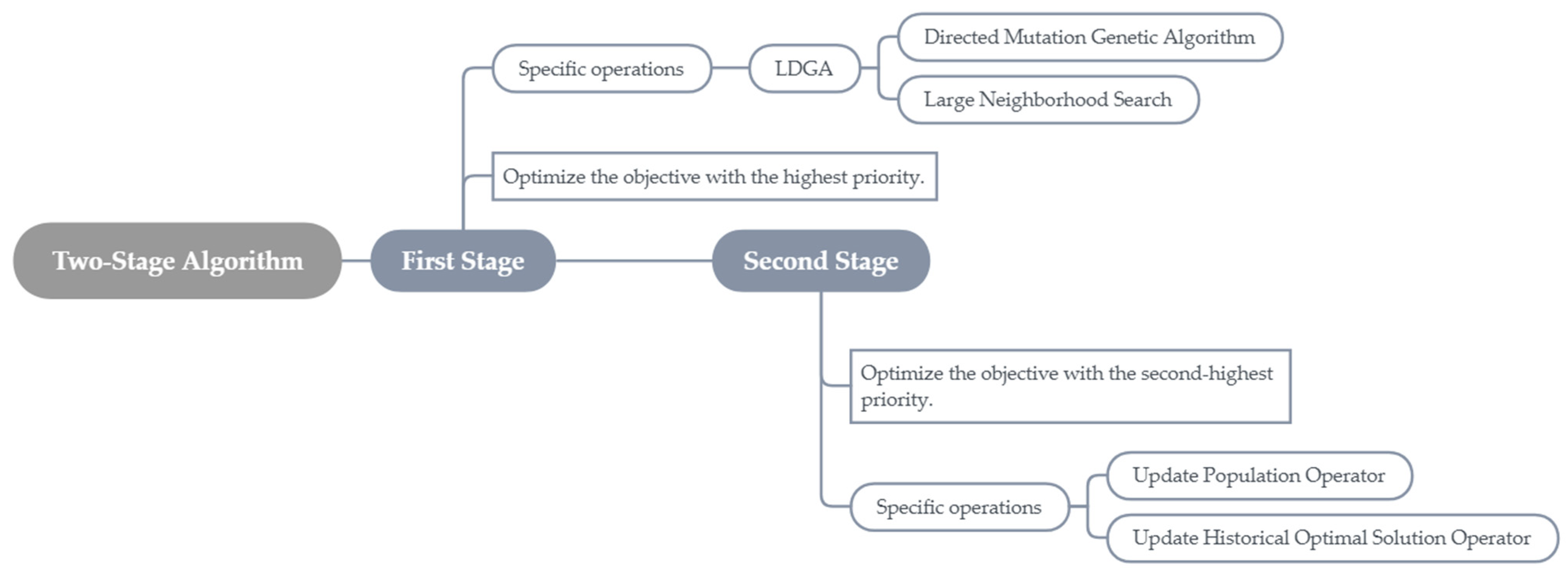
To address the multi-objective problem, this paper adopts a two-stage solution approach and discards the traditional method of using the optimal solution from the final generation of the population as the final solution in swarm intelligence algorithms. Instead, it defines a “historical optimal solution” variable and designs an algorithm that continuously updates this variable during the iteration process to seek Pareto solutions. Additionally, an updating operator for the population is designed to incorporate the “historical optimal solution”, resulting in excellent solving performance.

This paper designs two sets of algorithms to solve the VRPSFTW based on the principles of “cost priority” and “service-level priority”, respectively.

The general concept of the algorithm designed in this paper is illustrated in Figure 1.

3.1. Directed Mutation Genetic Algorithm

Below is a detailed introduction to the algorithm, including its chromosome encoding, initial population construction, fitness evaluation, chromosome selection, crossover, traditional mutation, and directed mutation.

3.1.1. Chromosome Encoding

In genetic algorithms, chromosome encoding is a way to represent the solutions to a problem as chromosomes. Each chromosome represents an individual (that is, a feasible solution). A chromosome is composed of a set of genes, and the population consists of a set of chromosomes.

The coding method adopted in this study treats the customer index numbers as the elements that constitute individuals (1, 2, 3, …, N), using a sequence of arranged customer index numbers to represent the customers served by a vehicle in order. The paths of all the vehicles in an overall delivery plan are concatenated to form a single individual code, and the index numbers of all the available vehicles are increased by N, resulting in a set, z = {1 + N, 2 + N, 3 + N, …, K + N}. The elements of set z are inserted sequentially between every two vehicle paths to indicate the vehicles’ return to the distribution center and to facilitate the distinction between different vehicle paths. If the length of the individual code has not reached N + K − 1, then elements from set z that have not been inserted between the two vehicle paths will continue to be added to the end of the code. When the length of the individual code reaches N + K − 1, the addition will stop.

For example, if the number of customers is 6, the customer index numbers are 1, 2, 3, 4, 5, 6, the maximum number of vehicles is 4, and the vehicle index numbers are 1, 2, 3, 4, then z = {1 + 6, 2 + 6, 3 + 6, 4 + 6} = {7, 8, 9, 10}. A feasible individual encoding can be represented as 127348569, where 7 and 8 indicate that a vehicle has completed its delivery and returned to the depot. The encoding is divided into three parts corresponding to the delivery routes of three vehicles, with 0 representing the depot, as follows:

0→1→2→0,

0→3→4→0,

0→5→6→0.

Because 9 is not inserted between the two vehicle paths, it is added to the end of the three routes. At this point, the length of the individual encoding has reached N + K − 1; thus, 10 is no longer added.

3.1.2. Initial Population Construction

In the genetic algorithm, the construction of the initial population directly impacts the convergence speed of the algorithm and its final optimization results. A good initial population can help the algorithm quickly find the global optimal solution, while a poor initial population is more likely to cause the algorithm to converge to a local optimal solution, or even fail to converge at all.

If the individuals in the initial population are somewhat close to the optimal solution, this will be more favorable for accelerating the convergence process. Therefore, the initial population construction method used in this study differs from the commonly used completely random construction. Instead, a heuristic method is employed, utilizing time window and vehicle load constraints to construct an initial population that satisfies these constraints as much as possible. The method is as follows:

Randomly generate a sequence $S$ that can traverse all customers, where each element $S\left[i\right]$ represents the customer index (i $\in$ {1, 2, 3, …, N}). Traverse each customer according to sequence $S$ and add them to the paths. The specific principles are as follows:

• Initialize a path, with the load of goods currently loaded by the vehicle on this path set as $l=0$;
• The current customer index being traversed is $S\left[i\right]$, the corresponding customer demand is $q$, and the maximum load capacity of each vehicle is $Q$;
• Determine whether inserting this customer into the current path satisfies the load constraint;
• When $l+q\le Q$, compare the start time ($a$) of the service window to find a suitable position to add the customer to the current path, for which there are three possible cases:
  • If the current path is empty, then simply add the customer to it;
  • If there is only one customer ($S[i-1]$) in the current path, compare the start time of the service windows ($a_{S\left[i\right]}$ and $a_{S[i-1]}$):

    a)

    If $a_{S\left[i\right]}$ is earlier than the start time of customer $S[i-1]$’s service window ($a_{S[i-1]}$), then insert customer $S\left[i\right]$ before $S[i-1]$;

    b)

    If $a_{S\left[i\right]}$ is later than the start time of customer $S[i-1]$’s service window ($a_{S[i-1]}$), then insert customer $S\left[i\right]$ after $S[i-1]$;

  • If there are multiple customers in the current path, then traverse their start times of their service windows:

    a)

    If $a_{S\left[i\right]}$ is earlier than the start time of the first customer in the path, then insert customer $S\left[i\right]$ at the beginning;

    b)

    If the interval between the start times of two adjacent customers in the path can accommodate $a_{S\left[i\right]}$, then insert customer $S\left[i\right]$ between them;

    c)

    If $a_{S\left[i\right]}$ is later than the start time of the last customer in the path, then insert customer $S\left[i\right]$ at the end;

• When $l+q\ge Q$, create a new path and insert customer $S\left[i\right]$ into it;
• Following the above steps, traverse from customer $S\left[1\right]$ to $S\left[n\right]$ to generate an initial solution;
• Repeat the above steps until initial solutions that meet the population size are generated.

3.1.3. Fitness Evaluation

In the “cost priority” algorithm, the fitness is the inverse of the cost function value, as follows:

$$Fitness={\displaystyle \frac{1}{f_1+f_2+f_3}}$$

(25)

In the “service-level priority” algorithm, the fitness is the overall service-level function value, as follows:

$$Fitness=\sum _{i=1}^n{q}_i{L}_i(\sum _{k=1}^K{y}_i^k{T}_{ik})$$

(26)

The fitness defined in this paper is primarily used for optimizing the solution of the first-priority objective in the first stage of a two-stage algorithm. The specific details of the two stages will be explained in more detail later.

3.1.4. Chromosome Selection

The roulette wheel selection method is employed in this study. In the genetic algorithm, roulette wheel selection is a commonly used selection strategy. Its basic idea is similar to selecting individuals on a rotating wheel, where the probability of each individual being selected is proportional to its fitness value. The advantage of this method is that it effectively preserves individuals with higher fitness, granting them a greater chance of survival, while it also considers individuals with lower fitness, thereby reducing the likelihood of falling into local optima to some extent.

3.1.5. Crossover

The crossover operator in the genetic algorithm simulates the gene exchange process in biological reproduction and evolution. Through the crossover operator, information between different individuals can be exchanged, resulting in new individuals. Specifically, the crossover operator exchanges part of the chromosome information (gene sequences) between two parent individuals to produce new offspring individuals. This way, there is a chance to combine the excellent characteristics of different individuals, resulting in better offspring.

The crossover method employed in this study is as follows: If two individuals, A and B, undergo a crossover operation, two crossover points are randomly selected, and the chromosome segments between these points form the crossover interval. The elements within the crossover interval are separately placed in front of the other individuals, resulting in new individuals, A’ and B’. Then, the new individuals are traversed from front to back for processing purposes; if duplicate elements are encountered, the second element is removed, leaving only the first one, which ensures that each element appears only once. Once these operations are complete, the crossover operation for individuals A and B is finished.

3.1.6. Traditional Mutation

The traditional mutation operation used in this study involves randomly selecting two genes on a chromosome and exchanging their positions.

3.1.7. Directed Mutation

This paper designs a directed mutation operator based on the traditional mutation operator, and the specific operation is as follows:

• Firstly, create a duplicate (b) of chromosome a.
• Perform the traditional mutation operation on duplicate b, generating b’.
• Compare the fitness levels of a and b’. If the fitness of b’ is better than that of a, replace a with b’; otherwise, retain a.

Unlike traditional mutation, the mutation rate of the directed mutation operator should be set higher. In this paper, it is set to 100%, meaning that all the individuals selected by the selection operator participate in the directed mutation.

3.2. Large Neighborhood Search

Large Neighborhood Search (LNS) is a heuristic search algorithm that is primarily used to solve combinatorial optimization problems (COPs). LNS explores the solution space by destroying and repairing parts of a solution, aiming to find better solutions.

The algorithm used in this study primarily applies the concept of destruction and repair from the LNS algorithm. Specifically, it involves removing a portion of the customers from the path and then re-inserting them.

3.2.1. Removal Operator

• Randomly select a customer from the path and remove it, then place it in the set μ.
• Randomly select a customer c from set μ.
• Calculate the relevance between the remaining customers in the path and customer c, then arrange these customers in temporary set α in descending order of their relevance to customer c. The function used to calculate the relevance is as follows:

  $$R(i,j)={\displaystyle \frac{1}{{d^{\prime }}_{ij}+D_{ij}}}$$

  (27)

  where ${d^{\prime }}_{ij}$ represents the normalized value of $d_{ij}$, with a range of [0, 1]. $D_{ij}$ represents whether i and j are on the same vehicle’s delivery route. If they are, $D_{ij}$ = 0; otherwise, $D_{ij}$ = 1.
• In order to avoid a situation wherein similar sets of visits are constantly selected based on relevance alone, a random element is added:

  $$RemoveIndex=Remain\times {rand}^P$$

  (28)

  where RemoveIndex represents the index of the next customer to be removed in set α; Remain represents the number of customers in set α; Rand represents a random number between 0 and 1; and P is the parameter controlling the determinism. When P = 1, relevance is ignored, and customers are randomly selected for removal from set α. When P = ∞, it approaches selecting the customer in set α with the highest rank (i.e., the customer most relevant to customer c) for removal.
• The removed customers are stored in set μ.
• Repeat steps B to E until the desired number of removed customers is met.

3.2.2. Re-Insertion Operator

The approach combines the farthest insertion heuristic with branch and bound.

• Take out an element from set μ, which is composed of removed customers.
• Find all the insertion points where inserting the element into the route satisfies the vehicle load constraint. If no such points exist, then create a new route and place the element into it.
• Calculate the increase in the distance that each feasible insertion scheme for the customer would bring to the total route, and identify the smallest increase in the distance among them.
• Perform the above operations for each element in the set μ. Find the element with the maximum “minimum distance increment” and insert it into the path according to the scheme with the smallest distance increment. Then, remove this element from the set μ.
• Repeat steps A to D until all the elements in the set μ are re-inserted into the route.

3.2.3. Acceptance Criterion

If the fitness value of the new solution is greater than that of the solution before the destruction and repair process, then accept the new solution as the current solution.

3.3. Directed Mutation Genetic Algorithm Combined with Large Neighborhood Search

To address the issue of high efficiency in the early stages but low efficiency in the later stages of the genetic algorithm, this paper proposes an algorithm that fully leverages the advantages of the genetic algorithm in the early stages while enhancing the search capability in the later stages. The specific combination approach of the algorithm is outlined as follows:

• In the early stage of the algorithm, only the traditional operations of the genetic algorithm are performed, adopting traditional mutation;
• When the algorithm iterates to the g-th generation, the population converges to a certain extent, and the speed of exploring the optimal solution slows down. At this point, directed mutation begins to replace traditional mutation;
• At the same time, a large neighborhood search removal operator and a re-insertion operator are added after the directed mutation operator;
• Starting from the g-th generation, the removal and re-insertion operations are performed every f generations. Finally, the removal and re-insertion operations are performed in every generation of the last h generations.

The parameters g, f, and h need to be reasonably set according to specific circumstances. The main consideration is the complexity of the problem, and the main factors that affect it are the number of points and their degree of clustering. If the problem is not very complex and requires fewer iterations to converge the population to a certain level, then g and f can be set smaller. If the problem is very complex, with a huge solution space, and requires more iterations to ensure that the algorithm has enough opportunities to explore the solution space, then g should correspondingly be set larger. It is an empirical summary that for datasets with around 100 points, when the number of iterations G is large (several thousand generations), balancing computational efficiency and effectiveness can be achieved by satisfying the following constraint:

$$20\le {\displaystyle \frac{G-g}{f}}+h\le 150$$

(29)

This constraint actually limits the number of executions of the removal and re-insertion operators used in the LDGA for solving datasets containing approximately 100 points. The reason is that these operators are effective but require a long execution time. When the number of executions is less than 20, their effectiveness is not fully realized and when the number of executions exceeds 150, the execution time becomes excessively long, and the marginal benefits decrease significantly in the later stages. Therefore, based on the experience gained from our experiments, we recommend limiting the number of executions to the range of [20, 150].

3.4. Operator for Determining the Start of the Service Time

According to the encoding method adopted in this study, a chromosome represents a delivery plan that can be decoded into multiple vehicle delivery routes. In this study, the planning of the start service time is carried out for each distribution route.

$t_{ik}$ represents the arrival time of vehicle k at customer i, and $T_{ik}$ represents the time at which vehicle k starts serving customer i. $route\left(i\right)$ represents the index of the i-th customer in the path among all the customers, where $a_{route\left(i\right)}$ is the desired start time of the service window for that customer, and $A_{route\left(i\right)}$ is the acceptable start time of the service window that the customer can tolerate.

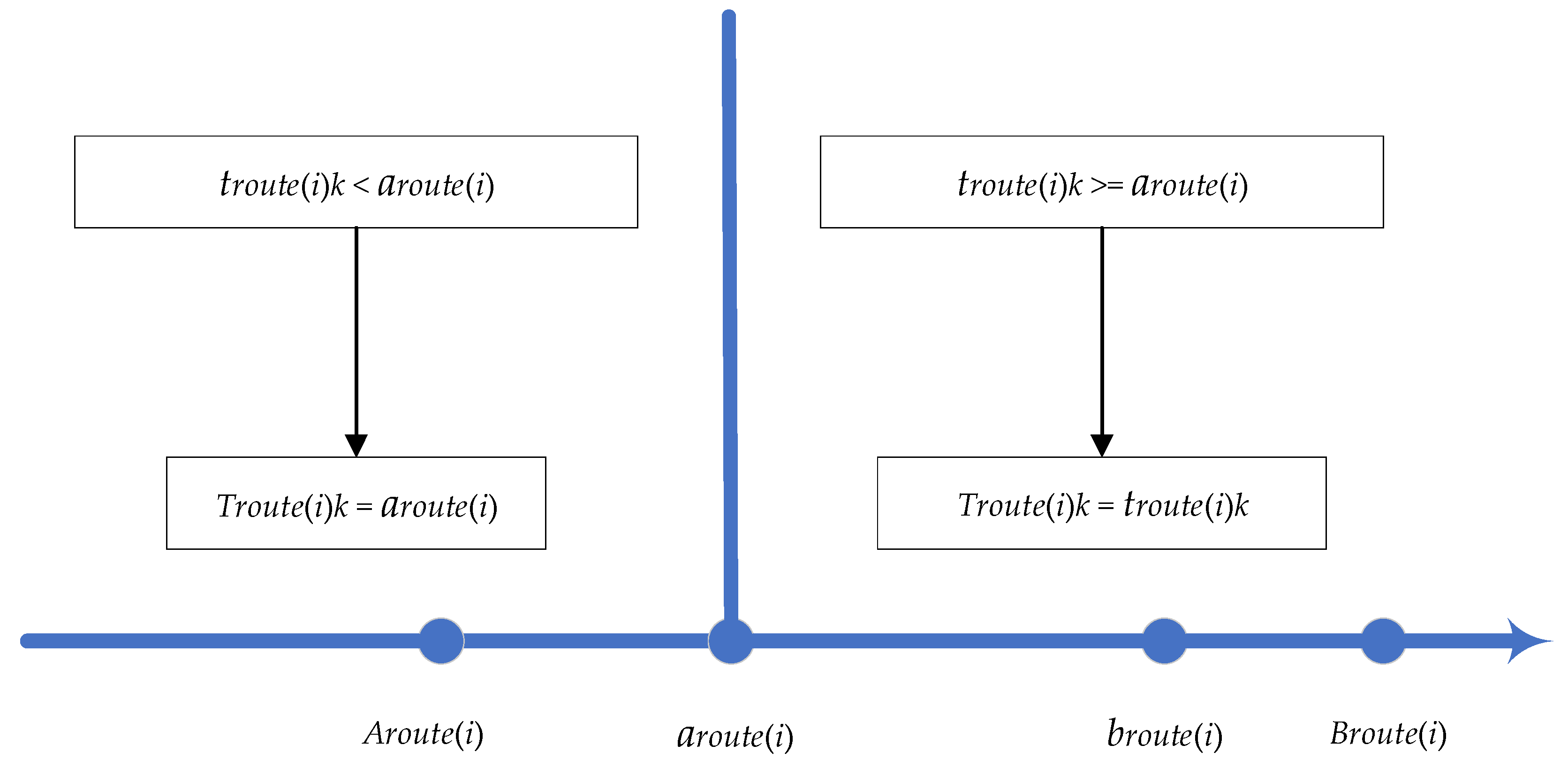
In the “cost priority” algorithm, the method for determining the start service time is as follows:

• Starting from the first customer served by vehicle k, calculate the arrival time ($t_{route\left(i\right)k}$) of vehicle k at that customer;
• If $t_{route\left(i\right)k}$ < $a_{route\left(i\right)}$, then execute the following operations:
  • Calculate the compensation cost of providing service to the customer in advance by one unit of time $BC=P_2\ast q_{route\left(i\right)}$, where $q_{route\left(i\right)}$ represents the demand of the i-th customer in that route;
  • $P_1$ is the waiting cost per unit time. Determine the relationship between $P_1$ and $BC$:

    a)

    If $P_1\le BC$, then $T_{route\left(i\right)k}=a_{route\left(i\right)}$;

    b)

    If $P_1>BC$, then determine which value is larger or smaller between $t_{route\left(i\right)k}$ and $A_{route\left(i\right)}$:

    • If $t_{route\left(i\right)k}\le A_{route\left(i\right)}$, then $T_{route\left(i\right)k}=A_{route\left(i\right)}$;
    • If $t_{route\left(i\right)k}>A_{route\left(i\right)}$, then $T_{route\left(i\right)k}=t_{route\left(i\right)k}$.

• If $t_{route\left(i\right)k}\ge a_{route\left(i\right)}$, then $T_{route\left(i\right)k}=t_{route\left(i\right)k}$.
• Repeat the process from A to C until all customers served by vehicle k have been traversed.

The idea behind the above operator is visually demonstrated in Figure 2.

In the “service-level priority” algorithm, the method for determining the start service time is as follows:

• Starting from the first customer served by vehicle k, calculate the arrival time ($t_{route\left(i\right)k}$) of vehicle k at the location of that customer;
• If $t_{route\left(i\right)k}<a_{route\left(i\right)}$, then $T_{route\left(i\right)k}=a_{route\left(i\right)}$;
• If $t_{route\left(i\right)k}\ge a_{route\left(i\right)}$, then $T_{route\left(i\right)k}=t_{route\left(i\right)k}$;
• Repeat the process from A to C until all customers served by vehicle k have been traversed.

The idea behind the above operator is visually demonstrated in Figure 3.

3.5. Update Historical Optimal Solution Operator

The previous operations mainly utilized the fitness function to screen and accept new solutions. In our algorithm, the “fitness function” is defined as “the objective function prioritized for optimization within the multi-objective function”. Therefore, the main role of the various operators in the preceding stage is to complete the optimization of the first phase in the two-stage algorithm. Updating the historical optimal solution is the core operation of the second stage of the two-stage algorithm and a key step in seeking Pareto solutions. This paper describes the specific operations of this operator in the two algorithms: “cost priority” and “service-level priority”.

The premise for updating the historical optimal solution is that a historical optimal solution is currently available. The operation for initializing the historical optimal solution follows immediately after the population initialization and before the iterative optimization. Taking “cost priority” as an example, it is first necessary to filter out the subset ${\mathrm{C}}_1$ of individuals in the initial population with the minimum total cost. Then, from ${\mathrm{C}}_1$, the subset ${\mathrm{C}}_2$ with the highest overall service level should be selected. Finally, we randomly choose one individual from ${\mathrm{C}}_2$ as the initial historical optimal solution. The “service-level priority” follows a similar approach: It is first necessary to filter out the subset of individuals with the highest overall service level. Then, from this subset, those with the minimum total cost should be selected. Finally, we randomly choose one individual from this group as the initial historical optimal solution.

In the “cost priority” algorithm, the method for updating the historical optimal solution is as follows:

• Calculate the cost function value of the current historical optimal solution ($BC$) and the overall service-level function value of the current historical optimal solution ($BSL$);
• Select the individuals with the minimum cost function values from the current population to form the set $Z_1$, and let their cost function values be $minC$;
• If $minC\le BC$:
  • If $minC=BC$:

    a)

    Select all individuals from $Z_1$ with an overall service level greater than $BSL$ to form the set $Z_2$;

    b)

    If $Z_2$ is non-empty:

    • Calculate the difference between the overall service level of each individual in set $Z_2$ and $BSL$, and identify all individuals with the largest difference to form the set $Z_3$;
    • Select any individual from set $Z_3$ as the new historical optimal solution;

    c)

    If $Z_2$ is empty, then retain the current historical optimal solution;

  • If $minC<BC$:

    a)

    Select any individual from set $Z_1$ to temporarily replace the historical optimal solution;

    b)

    Calculate the cost function value of the current historical optimal solution ($BC$) and the overall service-level function value of the current historical optimal solution ($BSL$);

    c)

    Select all individuals from $Z_1$ with an overall service level greater than $BSL$ to form the set $Z_2$;

    d)

    If $Z_2$ is non-empty, complete the following steps:

    • Calculate the difference between the overall service level of each individual in set $Z_2$ and $BSL$, and identify the individual with the largest difference to form the set $Z_3$;
    • Select any individual from set $Z_3$ as the new historical optimal solution;

    e)

    If $Z_2$ is empty, then retain the current historical optimal solution;

• If $minC>BC$, then retain the current historical optimal solution.

In the “service-level priority” algorithm, the method for updating the historical optimal solution is as follows:

• Calculate the cost function value of the current historical optimal solution ($BC$) and the overall service-level function value of the current historical optimal solution ($BSL$);
• Select the individuals with the maximum overall service-level function values from the current population to form the set $Z_1$, and let their overall service-level function values be $maxSL$;
• If $maxSL\ge BSL$:
  • If $maxSL=BSL$:

    a)

    Select all individuals from set $Z_1$ with cost function values less than $BC$ to form the set $Z_2$;

    b)

    If $Z_2$ is non-empty, complete the following steps:

    • Calculate the difference between $BC$ and the cost function value of each individual in set $Z_2$ and identify all individuals with the largest difference to form the set $Z_3$;
    • Select any individual from set $Z_3$ as the new historical optimal solution;

    c)

    If $Z_2$ is empty, then retain the current historical optimal solution.

  • If $maxSL>BSL$:

    a)

    Select any individual from set $Z_1$ to temporarily replace the historical optimal solution;

    b)

    Calculate the cost function value of the current historical optimal solution ($BC$) and the overall service-level function value of the current historical optimal solution ($BSL$);

    c)

    Select all individuals from set $Z_1$ whose cost function value is less than $BC$ to form set $Z_2$;

    d)

    If $Z_2$ is non-empty, complete the following steps:

    • Calculate the difference between $BC$ and the cost function value of each individual in set $Z_2$ and identify all individuals with the largest difference to form set $Z_3$;
    • Select any individual from set $Z_3$ as the new historical optimal solution;

    e)

    If $Z_2$ is empty, then retain the current historical optimal solution.

• If $maxSL<BSL$, then retain the current historical optimal solution.

3.6. Update Population Operator

In order to fully leverage the value of the superior individuals generated during the iteration process while ensuring the diversity of the population and avoiding local optimal solutions, the new population is composed of three parts: the current historical optimal solution, the new set of individuals generated during this iteration from the individuals selected by the selection operator, and a portion of the population from before this iteration. Firstly, the first two sets are added to the new population. Then, the individuals from the previous population are sorted in descending order based on their fitness values. Finally, a batch of individuals is selected from the sorted list and added to the new population until the number of individuals in the new population meets the specified criteria.

3.7. Two-Stage Algorithm

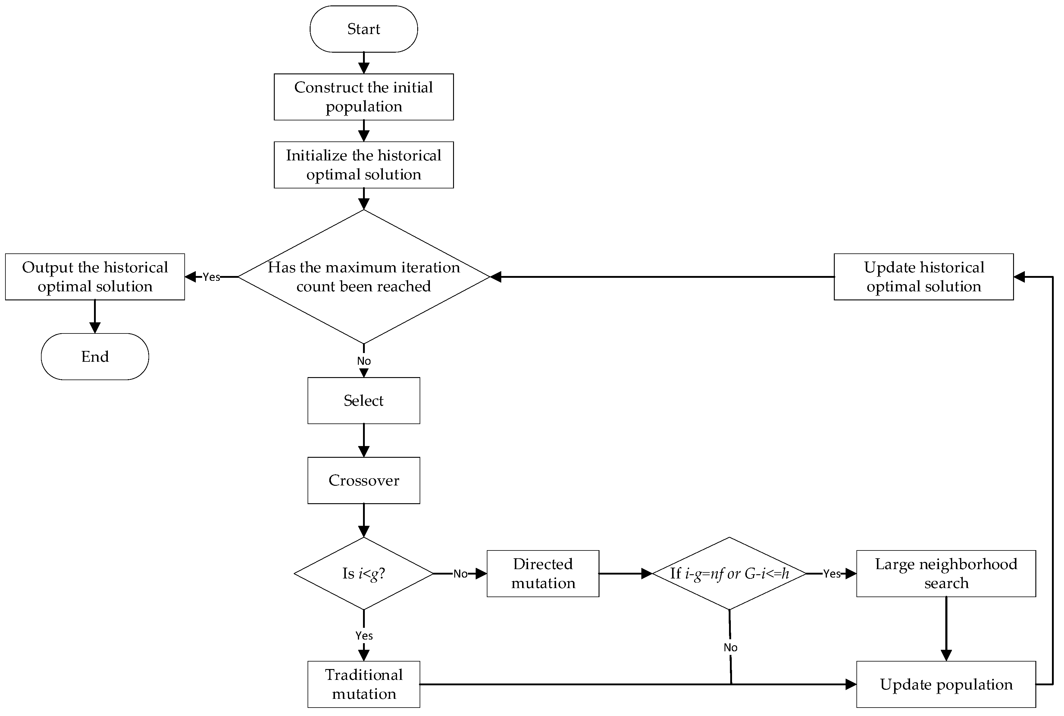
The first phase of the two-stage algorithm is primarily based on the Directed Mutation Genetic Algorithm combined with Large Neighborhood Search (LDGA), while the second phase focuses on the operator for updating the historical optimal solution.

Figure 4 presents a flowchart of the algorithm.

4. Experimental Results and Comparisons

4.1. Datasets Selection

To validate the effectiveness of our improved algorithm, this paper selected the classic Solomon benchmark test datasets for testing [26], and the relevant datasets can be accessed from “https://www.bernabe.dorronsoro.es/vrp/” accessed on 1 October 2024. Taking the first ten customer points and the depot from the C101 dataset as an example,

Table 1. The structure of the Solomon datasets.

Cust No.	Xcoord.	Ycoord.	Demand	${\mathit{a}}_{\mathit{i}}$	${\mathit{b}}_{\mathit{i}}$	Service Time
0	40	50	0	0	1236	0
1	45	68	10	912	967	90
2	45	70	30	825	870	90
3	42	66	10	65	146	90
4	42	68	10	727	782	90
5	42	65	10	15	67	90
6	40	69	20	621	702	90
7	40	66	20	170	225	90
8	38	68	20	255	324	90
9	38	70	10	534	605	90
10	35	66	10	357	410	90

shows the structure of the Solomon datasets.

The Solomon datasets can be divided into six categories: R1, C1, RC1, R2, C2, and RC2. In the R-class datasets, the coordinates of the nodes are randomly generated and relatively dispersed. In the C-class datasets, the coordinates form multiple clusters. In the RC-class datasets, the nodes are both random and clustered. Additionally, in the R1, C1, and RC1 datasets, the time intervals of each node’s time window are significantly smaller than those in the R2, C2, and RC2 datasets. This paper considered various scenarios and selected six representative datasets for testing and further development, as shown in

Table 2. Information on datasets (Scale represents the number of points in the dataset, including 1 distribution center and 100 customer points).

No.	Name	Scale	Vehicle Number	Capacity
1	C101	101	25	200
2	R101	101	25	200
3	RC101	101	25	200
4	C208	101	25	700
5	R208	101	25	1000
6	RC208	101	25	1000

.

To solve the problem model established in this paper, we expanded and constructed a set of datasets suitable for the VRPSFTW based on these six datasets, which were then used for the case testing. The classic Solomon benchmark test dataset does not include the $[A_i,B_i]$ values for customers. Therefore, this paper attempted to construct the $[A_i,B_i]$ values for each customer using the following formulas:

$$A_i=a_i-0.2\times rand\times a_i$$

(30)

$$B_i=b_i+0.2\times rand\times b_i$$

(31)

where $rand$ is a random number between 0 and 1. This is because if the weights are directly set as random numbers between 0 and 1, the resulting distribution may deviate too much, which does not align well with real-world delivery scenarios. Therefore, we chose to set the weights as random numbers between 0 and 0.2.

Table 3. The structure of the Extended Solomon dataset.

Cust No.	Xcoord.	Ycoord.	Demand	${\mathit{a}}_{\mathit{i}}$	${\mathit{b}}_{\mathit{i}}$	${\mathit{A}}_{\mathit{i}}$	${\mathit{B}}_{\mathit{i}}$	Service Time
0	40	50	0	0	1236	0	1236	0
1	45	68	10	912	967	907.52	1080.33	90
2	45	70	30	825	870	699.24	983.85	90
3	42	66	10	65	146	56.98	156.12	90
4	42	68	10	727	782	636.51	910.16	90
5	42	65	10	15	67	12.04	67.11	90
6	40	69	20	621	702	532.55	799.80	90
7	40	66	20	170	225	162.94	240.79	90
8	38	68	20	255	324	215.18	353.37	90
9	38	70	10	534	605	442.07	713.87	90
10	35	66	10	357	410	346.46	451.01	90

shows the structure of the Extended Solomon dataset using the first ten customer points and the depot from the Extended C101 dataset as an example.

In Section 4.2 and Section 4.3, this paper uses six datasets from the Solomon benchmark set to validate the effectiveness and superiority of the DGA and LDGA. The Solomon dataset is a typical set of test instances for the VRPTW and its variants and, to date, many studies have used these datasets for testing, making them a standard benchmark for related problems. Moreover, the six datasets we selected, which include R1, C1, RC1, R2, C2, and RC2, cover all the different types of instances with various characteristics in the Solomon dataset.

In Section 4.4, this paper uses a case study from Reference [27], which has been adopted in multiple studies. This case is well structured and corresponds to a typical multi-objective problem. We use this case to test the two-stage algorithm proposed in this paper to verify its effectiveness and superiority in solving multi-objective problems.

4.2. Effectiveness Validation of Directed Mutation

To verify the effectiveness of the directed mutation operator in solving the VRPTW, this paper compared the Directed Mutation Genetic Algorithm (DGA) to the Standard Genetic Algorithm (SGA). The Solomon benchmark datasets were used for testing.

In the C-class datasets, the coordinates form multiple clusters; in the R-class datasets, the coordinates of the nodes are randomly generated and relatively dispersed; and in the RC-class datasets, the nodes are both random and clustered. Therefore, for the C-class datasets, the population can converge to a satisfactory level with relatively fewer generations, and for the R- and RC-class datasets, more generations are required to achieve convergence at a satisfactory level. A large number of experiments were conducted in this study to better set the number of iterations. Due to the paper’s length, this paper presents only the convergence curves of two representative datasets, as shown in Figure 5.

As shown in Figure 5, the C208 convergence curve shows little change when the number of iterations reaches 3000, and in our experiments, the other C-class datasets exhibited similar behavior. The RC208 convergence curve still decreases after 3000 iterations, stabilizing around 4000 generations. Similarly, the other R-class and RC-class datasets in our experiments exhibit the same pattern. Therefore, for the C-class datasets, the number of iterations was set to 3000, and for the R- and RC-classes, it was set to 4000. The algorithm with the directed mutation operator replaced traditional mutation with directed mutation starting from the 2000th generation until the end of the iterations. The population size was 100, the generation gap (the proportion of individuals selected by the selection operator relative to the total number of individuals in the population) was 0.9, the crossover probability was 0.9, and the directed mutation probability was 1. Through extensive research, we found that the mutation rates are typically set within the range of 0.01 to 0.2 and should not be too high or too low. We conducted numerous experiments, starting with a mutation rate of 0.01 and increasing it by 0.005 each time until we reached 0.2, testing each mutation rate 10 times. We selected the best-performing mutation rate, 0.05, as the traditional mutation probability. Each algorithm was run 10 times for each dataset to ensure the reliability of the experimental data, and the experimental results are shown in

Table 4. Comparison of DGA and GA solutions.

Instance	Best-Known Distance	Average		Min		Variance		Relative Error
		DGA	SGA	DGA	SGA	DGA	SGA	DGA	SGA
C101	828.94	1153.44	1289.83	1019.46	1155.36	7986.78	8075.72	0.39	0.56
R101	1650.8	1808.61	1940.11	1751.80	1795.48	1591.88	8372.87	0.10	0.18
RC101	1696.95	1912.04	2002.48	1873.73	1903.60	1806.55	3712.27	0.13	0.18
C208	588.32	780.85	855.91	727.21	745.79	1163.29	5794.91	0.33	0.45
R208	726.82	1032.02	1176.10	972.67	1092.83	1614.68	2848.17	0.42	0.62
RC208	828.14	1182.76	1332.47	1134.07	1222.76	1825.95	4790.37	0.43	0.61

.

The formula for calculating the relative error is as follows:

$$Relative Error={\displaystyle \frac{Average Value-Best Known Distance}{Best Known Distance}}$$

(32)

The average computation time per generation of the SGA is 0.1254 s. For the C-class datasets, the DGA runs for 3000 generations, with an average computation time of 0.1265 s per generation. For the R- and RC-class datasets, the DGA runs for 4000 generations, with an average computation time of 0.1560 s per generation.

According to the experimental results for the six representative datasets, the results of the DGA in terms of the mean, minimum, relative error, and variance are superior to those of the SGA, proving the effectiveness of the directed mutation operator and the superiority of the DGA.

4.3. Comparison of LDGA with Other Algorithms

To validate the effectiveness and superiority of the Directed Mutation Genetic Algorithm combined with Large Neighborhood Search (LDGA) for solving the VRPTW, it was compared against recently published representative algorithms, including the hybrid swarm intelligence algorithm which was created by hybridizing Ant Colony System and Brain Storm Optimization algorithm (BSO), the Multi-Objective Large Neighborhood Search algorithm (MOLNS), and Neighborhood Comprehensive Learning Particle Swarm Optimization (N-CLPSO). For the C-class datasets, this paper sets the number of iterations for the LDGA to 3000. Starting from the 2000th generation, this paper performs removal and re-insertion operations every 100 generations, with the final 10 generations executing these operations in every iteration. For the R- and RC-class datasets, this paper sets the number of iterations for the LDGA to 4000. Starting from the 2000th generation, this paper performs removal and re-insertion operations every 50 generations, with the final 100 generations executing these operations in every iteration. In the removal operator, the parameter controlling the determinism ($P$) is set to 15, and the number of customers to be removed is set to 15. Other parameters are set as described in Section 4.2. The experimental results are shown in

Table 5. Comparison of LDGA with other algorithms.

Instance	Best-Known Distance	Algorithm				Comparison with the Best-Known Distance
		LDGA	BSO	MOLNS	N-CLPSO	LDGA	BSO	MOLNS	N-CLPSO
C101	828.94	828.94	828.94	828.94	828.94	=	=	=	=
R101	1650.80	1646.05	1671.16	1654.93	1648.08	−4.75	+20.36	+4.13	−2.72
RC101	1696.95	1657.37	1643.78	1662.56	1635.11	−39.58	−53.17	−34.39	−61.84
C208	588.32	588.32	588.32	588.32	588.32	=	=	=	=
R208	726.82	722.84	940.30	754.99	740.36	−3.98	+213.48	+28.17	+13.54
RC208	828.14	802.43	910.59	859.13	843.28	−25.71	+82.45	+30.99	+15.14

.

According to Table 5, the LDGA achieved better results than the other algorithms in four out of the six datasets tested. Additionally, the LDGA achieved results consistent with the best-known distance in the C-class datasets and even surpassed the best-known distance in the R- and RC-class datasets. In conclusion, the experimental results demonstrate the superiority of the LDGA in exploring the solution space.

The vehicle transport route solutions for the six instances computed using the LDGA are shown in Figure 6.

4.4. Comparison of the Two-Stage Algorithm with NSGA-II

To validate the effectiveness and superiority of the two-stage algorithm proposed in this paper for solving multi-objective problems, this section conducted simulation experiments using the test cases from Reference [27] and compared the results with the popular NSGA-II. The specific details of the cases are as follows: A single distribution center serves multiple customers, with the center located at the central position relative to all the customers, numbered as 0, and the customer distribution is radial. All the delivery vehicles are of the same specifications, with a maximum load capacity of 8 tons, an average speed of 40 km/h, a fixed vehicle cost of CNY 100, and a travel cost of CNY 2 per kilometer. The waiting cost is CNY 10 per hour, and the penalty cost is CNY 40 per hour.

Table 6. A portion of the customer information.

Cust No.	Xcoord.	Ycoord.	Demand	${\mathbf{a}}_{\mathbf{i}}$	${\mathbf{b}}_{\mathbf{i}}$	${\mathbf{A}}_{\mathbf{i}}$	${\mathbf{B}}_{\mathbf{i}}$	Service Time
0	70	70	0	0	10	0	10	0
1	107	77	3.4	1.5	3.5	0.5	4.5	0.2
2	109	139	0.8	3	5.5	2	6.5	0.2
3	120	22	3.9	2	5	1	6	0.2
4	48	47	1.9	1.5	5	0.5	6	0.4
5	116	22	3.2	2	5.5	1	6.5	0.2
6	12	138	1.4	4	8	3	9	0.5
7	86	40	2.2	1.5	3	0.5	4	0.4
8	121	124	2.1	2.5	5	1.5	6	0.2
9	61	57	3.5	4.5	8	3.5	9	0.2
10	40	113	2.3	2	3.5	1	4.5	0.2

shows a portion of the customer information.

The parameter settings are as follows: the population size is 100, the generation gap is 0.9, the crossover probability is 0.9, and the traditional mutation probability is 0.05. Starting from the 2000th generation, directed mutation replaces traditional mutation with a probability of 1. A removal and re-insertion operation is performed every 50 generations, and in the last 100 generations, this operation is executed in each generation. In the removal operator, the deterministic parameter is set to $P=15$, and the number of customers to be removed is set to 15. The problem model and relevant parameters are consistent with those in Reference [27]. The aims of the objective functions in this reference are to minimize the total cost and maximize the average customer satisfaction. The satisfaction of a single customer ranges within [0, 1], and the average customer satisfaction function is the geometric mean of the satisfaction levels of all the customers, with a maximum value of 1. The experimental results are shown in

Table 7. Comparison of two-stage algorithm and NSGA-Ⅱ solutions.

	Two-Stage Algorithm				NSGA-Ⅱ
	Best	Average	Worst	SD	Best	Average	Worst	SD
Minimum Cost	2627.61	2629.90	2633.57	3.21	2636.42	2728.66	2860.91	224.49
Maximum Satisfaction	1	1	1	0	0.87	0.76	0.65	0.22

.

The experimental results indicate that for this multi-objective problem, the two-stage algorithm proposed in this paper significantly outperforms the NSGA-II in terms of the best, average, and worst values, as well as in terms of the standard deviation of the minimum cost and maximum satisfaction. This demonstrates that our algorithm has a clear advantage in handling priority objectives. In situations with limited resources and clearly defined priority goals, the algorithm can effectively address the key objectives while optimizing the secondary objectives to the best of its ability. This mechanism makes the algorithm more aligned with the demands of practical applications.

The two transportation route schemes calculated using the two-stage algorithm for this case are shown in Figure 7.

4.5. Results of the Two-Stage Algorithm for Solving the VRPSFTW

This paper considers real-world scenarios and integrates improvements to the VRPSTW and VRPFTW, establishing a multi-objective vehicle routing problem model known as the VRPSFTW, which incorporates soft and fuzzy time windows. This section will apply the two-stage algorithm designed in this study to solve this problem. A simulation experiment is conducted using the Solomon datasets extended in Section 4.1.

The model parameter settings are shown in

Table 8. The model parameter settings.

Vehicle waiting cost coefficient	$P_1=0.2$ CNY/min
Penalty coefficient for starting service early	$P_2=0.01$ CNY/min
Penalty coefficient for delaying service	$P_3=0.02$ CNY/min
Fixed cost per vehicle	F = 60 CNY
Average vehicle speed	v = 60 km/h
Unit travel cost	p = 1 CNY/km

.

The maximum number of vehicles and the maximum load capacity per vehicle are as specified in Table 2, and the algorithm parameters are the same as those in Section 4.4.

The results of the two-stage algorithm for solving the VRPSFTW are shown in

Table 9. Computational results of the VRPSFTW.

Cost Priority
Instance	Historical Minimum Cost	Corresponding Maximum Service Level	Driving Distance	Number of Vehicles Used	Computation Time
					Total(s)	Per Generation(s)
Extended C101	2955.6796	1644.4137	1714.6901	14	1511.1317	0.5037
Extended R101	2995.5166	603.2438	1541.2318	12	1546.2189	0.3866
Extended RC101	3001.2132	997.9049	1520.7091	12	1578.7034	0.3947
Extended C208	1483.3169	1772.1749	1151.3776	4	1396.5394	0.4655
Extended R208	1080.574	1355.992	794.314	3	1544.5854	0.3861
Extended RC208	1433.8688	1574.0623	873.7282	4	1395.6434	0.3489
Service-level priority
Instance	Historical Maximum Service Level	Corresponding Minimum Cost	Driving Distance	Number of Vehicles Used	Computation Time
					Total(s)	Per Generation(s)
Extended C101	1810	4087.5234	2289.3963	18	1772.7931	0.5909
Extended R101	1423.2651	4601.7969	2807.3128	25	1823.4569	0.4559
Extended RC101	1700.615	4639.1321	2920.7883	25	1828.9712	0.4572
Extended C208	1810	4453.73	2541.884	7	1626.1256	0.5420
Extended R208	1458	2690.5842	1866.3872	8	1631.2378	0.4078
Extended RC208	1724	3910.9925	2908.1711	10	1690.4991	0.4226

.

This paper obtained two sets of results using two algorithms designed based on the “cost priority” and “service-level priority” principles. For the same case, the final results from the “cost priority” algorithm showed significantly lower costs compared to those of the “service-level priority” algorithm, while also optimizing the service levels to some extent. In this approach, the service quality is not neglected in the pursuit of the lowest cost. Conversely, the final results from the “service-level priority” algorithm demonstrated significantly higher service levels than those obtained from the “cost priority” algorithm, while also achieving some degree of cost optimization. This helps prevent resource wastage that could arise from focusing solely on service level maximization without considering cost control. Decision-makers can flexibly choose a solution strategy based on their actual needs to better achieve their objectives.

The transportation route schemes obtained from solving three of these cases using the two-stage algorithm are shown in Figure 8.

The cost priority algorithm solving the Extended C101 is used as an example to illustrate the operation of our algorithm. Figure 9 shows the iterative evolution of the two objective function values.

As can be seen from Figure 9, under the cost priority strategy, the total cost function continuously decreases during the iteration process, while the total service-level function fluctuates within a small range but shows an overall increasing trend. This indicates that both objective functions have been effectively optimized during the iteration process.

Finally, Figure 10 displays the scatter plot of the two objective functions.

As shown in Figure 10, the cost decreases while the service level increases during the iteration process, which means that both objective functions have been optimized during the iteration process, demonstrating the effectiveness of the two-stage algorithm designed in this study for solving the VRPSFTW.

Due to the paper’s length, this paper presents only a selection of these representative datasets; however, we also tested other datasets, including numerous VRPTW-related cases from the website “https://www.bernabe.dorronsoro.es/vrp/” accessed on 1 October 2024, and the algorithms proposed in this paper also demonstrated excellent performances in solving these cases.

5. Conclusions

This paper established a vehicle routing problem with soft time windows and fuzzy time windows (VRPSFTW) and designs a two-stage heuristic algorithm to solve the VRPSFTW.

The VRPSFTW established in this study represents a synthesis and extension of the VRPSTW and VRPFTW, incorporating the strengths of both models while addressing their shortcomings.

This paper has improved the mutation operation of traditional genetic algorithm in the LDGA by proposing a directed mutation operator, while also integrating a large neighborhood search algorithm, enhancing the search capability of the algorithm in the later stages. The overall algorithm design fully utilizes the advantages of the genetic algorithm in the early stages. In the middle and later stages, directed mutation is used instead of traditional mutation, and removal and re-insertion operators are introduced to compensate for the weakness of the genetic algorithm in the later stages, thereby improving its overall efficiency and accuracy. The experimental results indicate that the LDGA is significantly competitive in exploring the solution space among the selected state-of-the-art algorithms recently published.

For multi-objective problems, the two-stage algorithm designed in this paper significantly outperforms the NSGA-II in handling priorities among objectives. Under conditions of limited resources and clearly defined primary goals, the algorithm can effectively optimize the key objectives while also addressing the secondary objectives within feasible limits. This mechanism makes the algorithm more aligned with the demands of practical applications.

The implications of this paper for relevant business managers in reality are as follows:

(1)

The VRPSFTW model is more effective at describing the real-world scenarios faced by managers who have access to customer-related information. This model simultaneously considers two objective functions: total cost and total service level. This not only enables managers to optimize both the company’s short-term and long-term profits when designing delivery plans, but also helps improve customer satisfaction, achieving a win–win situation for both the company and its clients. Moreover, the model provides a more accurate and reasonable characterization of total cost and total service level, allowing managers to better understand the actual impact of the related delivery plans and thus make more informed vehicle routing decisions.

(2)

The LDGA provides a valuable tool that management decision-makers in relevant enterprises can consider for optimizing vehicle routing arrangements.

(3)

In reality, management decision-makers often have limited resources and typically have clear priority optimization goals during specific periods. Therefore, they can use the two-stage algorithm and flexibly choose solution strategies based on their actual needs to better achieve their objectives:

1)

When the company is in a phase that requires prioritizing cost savings, decision-makers can use the two-stage algorithm with the cost priority strategy for vehicle routing. This approach aims to minimize cost while also optimizing the service level to a certain extent, thereby avoiding any neglect of the service level due to a sole focus on cost reduction.

2)

When the company is in a phase that requires prioritizing customer satisfaction, decision-makers can use the two-stage algorithm with the service-level priority strategy for vehicle routing. This approach aims to maximize the service level while also optimizing cost to some extent, thereby avoiding any neglect of cost control that could lead to resource waste due to a sole focus on the service level.

Although the algorithm designed in this study demonstrates excellent performance, there is still room for further improvement. In our algorithm structure, the timing and frequency of the use of various operators are derived from empirical summaries based on multiple experiments. We hope to establish more standardized rules or develop adaptive rules that can be adjusted according to the population conditions in future research, which could potentially enhance the overall performance of the algorithm. Furthermore, the operator we designed to determine the starting service time employs a greedy strategy, which may not guarantee an optimal solution, which warrants further investigation.