Layout Planning of a Basic Public Transit Network Considering Expected Travel Times and Transportation Efficiency

Abstract

Urban transit systems are crucial for modern cities, providing sustainable and efficient transportation solutions for residents’ daily commutes. Extensive research has been conducted on optimizing the design of transit systems. Among these studies, designing transit line trajectories and setting operating frequencies are critical components at the strategic planning level, and they are typically implemented in an urban integrated transportation network. However, its computational complexity grows exponentially with the expansion of urban integrated transportation networks, resulting in challenges to global optimization in large-scale cities. To address this problem, this study investigates the layout planning of a basic public transit network (BPTN) to simplify the urban integrated transportation network by filtering out road segments and intersections that are unattractive for both users and operators. A non-linear integer programming model is proposed to maximize the utility of the BPTN, which is defined as a weighted sum of expected travel times (from a user perspective) and transportation efficiency (from an operator perspective). An expected transit flow distribution (ETFD) analysis method is developed, combining different assignment approaches to evaluate the expected travel time and transportation efficiency of the BPTN under various types of transit systems. Moreover, we propose an objective–subjective integrated weighting approach to determine reasonable weight coefficients for travel time and transportation efficiency. The problem is solved by a heuristic solution framework with a topological graph simplification (TGS) process that further simplifies the BPTN into a small-scale graph. Numerical experiments demonstrate the efficacy of the proposed model and algorithm in achieving desirable BPTN layouts for different types of transit systems under variable demand structures. The scale of the BPTN is significantly reduced while maintaining a well-balanced trade-off between expected travel time and transportation efficiency.

1. Introduction

Urban transit systems are crucial for modern cities, providing sustainable and efficient transportation solutions for residents’ daily commutes. As summarized by Ceder and Wilson [1], the overall planning of urban transit systems primarily involves the following five tasks: (1) planning public transit routes, (2) setting route operational frequencies, (3) formulating operational timetables, (4) scheduling buses, and (5) scheduling drivers. Among these, designing route trajectories and setting their operating frequencies are critical components at the strategic planning level that are typically implemented in an urban integrated transportation network [2,3,4,5,6,7,8]. However, an urban integrated transportation network contains numerous nodes and edges, such as road segments, intersections, rail segments, rail stations, and pedestrian paths. Despite the existence of numerous modeling methods and solution algorithms in previous studies, it has been demonstrated that the computational complexity of the transit route trajectory design and frequency setting problem grows exponentially as the integrated network scale expands. Consequently, achieving global optimization becomes challenging in large-scale networks.

To efficiently address planning challenges in large-scale public transit systems, it is necessary to simplify the integrated network and convert it into a topology graph, thereby significantly reducing its computational complexity. In other words, the purpose of integrated network simplification is to determine the layout of a basic public transit network (BPTN) by filtering out road segments and intersections that are unattractive for both users and operators. Topology graph simplification (TGS) aims to identify critical nodes within the BPTN that can potentially serve as transfer hubs while utilizing edges to represent associated road segments that connect transfer and centroid nodes. However, there is a trade-off between the coverage and efficiency of a BPTN. A small-scale, aggregated BPTN may overlook valuable road segments that are pivotal for transit route deployment, while a large-scale, dense BPTN is less efficient in addressing route trajectory design and frequency setting problems. The challenges of balancing coverage and efficiency in determining an expected BPTN that aligns with the demand structure, as well as conducting TGS to identify critical nodes and edges, are both significant issues to be addressed.

1.1. Literature Review

The foundation of transportation system planning lies in network layout optimization and graph theory. In 1975, an early work by Christofides [9] on the minimum spanning tree and shortest path problems set the stage for modeling network layout optimization. Optimization models are essential for determining the most efficient network layouts that balance cost, coverage, and service quality. In 1979, Garey and Johnson [10] highlighted the computational complexity associated with various optimization problems in network layout design, emphasizing the need for heuristic and approximation algorithms. Papageorgiou, Toth, and Vigo [11] discussed advanced optimization techniques, including integer programming and metaheuristics, which are pivotal for solving large-scale transit network design problems. In 2005, Diestel [12] provided a comprehensive overview of graph theory, emphasizing concepts like connectivity, traversability, and network flows, which are directly applicable to network layout design.

When focusing on transit network layout planning, previous studies have extensively examined three classical layout patterns (e.g., hub-and-spoke, grid, and hybrid) with regard to their coverage, accessibility, and operational efficiency. O’Kelly [13] introduced the concept of hub-and-spoke systems and emphasized the importance of central hubs in reducing travel time and operational costs in transportation networks. This model has been widely applied in both urban and intercity transit systems. In 2005, Vuchic [14] distinguished between different network layouts, such as hub-and-spoke, grid, and hybrid networks. Hub-and-spoke networks, where routes converge on a central point, are effective for central business district-focused cities. However, their accessibility diminishes when the city has multiple activity centers or decentralized development. In contrast, grid networks, which offer multiple intersecting routes covering a city, are more effective in providing uniform accessibility across urban areas but will reduce operational efficiency [15]. In 2010, Daganzo [16] explored the adaptability of hybrid network layouts, demonstrating their abilities to balance the coverage and accessibility advantages of grid layouts and the operational efficiency benefits of hub-and-spoke layouts, thereby accommodating both high-density and low-density urban areas. In addition, some studies investigated the effects of different network layouts on users’ travel costs. Thompson and Matoff [17] found that grid-based layouts, which provide extensive coverage, tend to offer lower travel costs for short trips but can result in higher costs for longer trips due to the need for multiple transfers. Conversely, hub-and-spoke layouts, which focus on connecting suburbs to the central city, often minimize travel costs for longer trips but offer limited coverage for intra-suburban travel. Nourbakhsh and Ouyang [18] considered the agency and user cost of a flexible transit system and optimized the transit network layout in idealized square cities to minimize the total system cost.

In fact, as the foundation of transportation, the urban integrated transportation network plays a significant role in determining transit system performance [19]. It has been found that a lower connectivity of a road network results in a lower supply of public transportation, thereby promoting the utilization of private cars [20]. In contrast, enhanced connectivity and a pedestrian-friendly integrated transportation network has the potential to provide a high-quality transit system that attracts greater usage by residents [21]. Regarding the design of transit line trajectories and setting of operating frequencies, most studies [3,4,5] are conducted based on existing urban integrated transportation networks with a focus on aligning with demand structures rather than being constrained by fixed layout patterns. However, due to the complexity and NP-hardness of the problem, effectively addressing the problem in large-scale urban transportation systems remains a formidable challenge. Therefore, it is necessary to simplify the integrated transportation network by filtering out road segments and intersections that are unsuitable for deploying transit lines and unattractive for both users and operators, resulting in a BPTN layout that optimizes benefits for all stakeholders. In recent years, extensive studies have focused on simplifying complex networks and analyzing critical elements of complex networks using graph theory. For example, De Bona et al. [22] introduced a reduced model as a straightforward approach for network reduction, effectively preserving the network skeleton by removing two-degree nodes of weighted and unweighted network representations. Bontorin et al. [23] proposed a simple model for BPTN generation in which a network lattice is utilized as a planar substrate and edge speeds are employed to define an effective temporal distance for optimizing and quantifying the efficiency of urban space exploration. Polimeni and Vitetta [24] modeled the network design problem in road transport systems to minimize congestion and the impacts on the network from passengers. A heuristic algorithm is developed to find the best network configuration. Wang et al. [25] proposed a geospatial network analysis method to investigate the spatial configuration of an urban bus network. Shanmukhappa et al. [26] analyzed bus transport network structures by considering network spatial embedding for three cities, namely Hong Kong, London, and Bengaluru. By utilizing a super node graph approach, they successfully examined essential network parameters for directed, weighted, and geo-referenced bus transport networks. Tian et al. [27] analyzed the land use and characteristics of road networks and utilized topology modeling theory to identify the hierarchies of transit corridors. Badia et al. [28] proposed an analytical model to optimize the BPTN layout with radial street patterns. The objective function was to minimize the total cost of agency and users. Fan et al. [29] optimized an intersecting bimodal BPTN layout including sparse express and dense local networks based on cities with grid street patterns. In summary, despite the extensive progress made in previous studies, there remains a gap in the literature regarding how to simplify the urban integrated transportation network and achieve an appropriate BPTN layout that aligns with the transit demand structure while benefiting both users and operators.

1.2. Objective and Contribution

In this study, we investigate the layout planning problem to extract a BPTN from the urban integrated transportation network, as well as a TGS method to convert the BPTN into a topology graph. The objective of this study is to filter out unnecessary road segments and intersections and obtain BPTN layouts that align with the interests of users and operators; then, we recognize potential transfer stations within the BPTN and convert it into a topological graph. By implementing the layout planning of the BPTN and TGS, we can achieve a simplified topological graph with a limited number of edges and nodes that are attractive for both users and operators, thereby facilitating the global optimization design of subsequential transit line deployment or other strategic and tactical decisions for transit systems.

To achieve these objectives, we propose a non-linear integer programming model to maximize the utility of the BPTN, which is formulated as the weighted sum of total expected travel time for users and the transportation efficiency for operators within the BPTN. Considering the level of the transit system to be planned, we propose a method to estimate the expected transit flow distribution (ETFD) under a given BPTN, thereby providing essential information for evaluating the total expected travel time and transportation efficiency. An entropy-based and subjective integrated weighting method is proposed to determine reasonable weight coefficients for the travel time and transportation efficiency, respectively. Moreover, a heuristic solution framework is proposed to solve the proposed BPTN layout planning and TGS problems. Numerical results based on a real urban integrated transportation network are presented to demonstrate the efficacy of the proposed model and solution framework.

The remainder of this paper is organized as follows: Section 2 introduces the notations, assumptions, problem description, and the overall solution framework; Section 3 elucidates the ETFD analysis method involved in the solution framework; Section 4 presents the entropy-based and subjective integrated weighting method, as well as the TGS method; Section 5 details a case study; and Section 6 presents the conclusions.

2. Notations, Assumptions, Problem Description, and Solution Framework

We define the BPTN layout planning problem over an urban integrated transportation network denoted as $G^0=(N^0,A^0)$, where $N^0$ is the set of nodes including intersections and centroid nodes of traffic zones, and $A^0$ is the set of road segments. The set of origin–destination (OD) pairs in the network is denoted as $W≔\left\{w=\left(i,j\right)|i,j\in N^0\right\}$, and the public transit travel demand between a given OD pair is denoted as $q_w$, $\forall w\in W$. In addition, the expected travel time for public transit service on each road segment is represented by $t_a$, $\forall a\in A^0$. Since any connected subgraph containing all centroid nodes can be represented as a combination of paths connecting each OD pair, let $K_w$ denote the set of candidate paths connecting the OD pair $w$ and $\prod _{w\in W}{K}_w=\left\{\mathcal{k}:W\to {\bigcup }_{w\in W}{K}_w|\forall w\in W,\mathcal{k}\left(w\right)\in K_w\right\}$ denote the Cartesian product of the indexed family of sets ${\left\{K_w\right\}}_{w\in W}$. Then, the objective of the BPTN layout planning problem is to determine a combination of paths connecting each OD pair, denoted by $\mathcal{k}\in \prod _{w\in W}{K}_w$, that can maximize its overall utility. In this study, the utility of the BPTN is defined as the weighted sum of expected travel time and transportation efficiency of selected paths between each OD pair. In addition, the TGS is to simplify the path combination $\mathcal{k}$ and convert it into a topological graph $G=(N,A)$ by identifying potential transfer nodes and merging head-to-tail road segments. Here, $G$ is a subgraph of $G^0$, $N$ is a subset of $N^0$, and $A$ is a subset of $A^0$.

Figure 1 shows an example of the BPTN layout planning and TGS. The selected paths connecting each OD pair result in a BPTN that is a sub-network of the integrated transportation network; then, the TGS converts the BPTN into a topological graph, with the traffic zone centroids and potential transfer hubs as nodes and merged road segments on selected paths as edges. This process significantly reduces the network scale and facilitates the global optimization design of transit line deployment in large cities. As shown in Figure 1, the number of intersections and road segments in the integrated transportation network is 100 and 220, respectively. After the BPTN layout planning, the number of intersections and road segments reduces to 30 and 33, respectively. Moreover, the topological graph generated by TGS effectively reduces the number of nodes and edges to 7 each.

Figure 2 illustrates two distinct layout configurations of the BPTN, wherein the region is partitioned into four traffic zones with centroid nodes denoted as A, B, C, and D. The BPTN depicted in Figure 2a comprises the shortest paths between adjacent centroid nodes. However, for the non-adjacent OD pairs AD and BC, travel paths require passing through other centroid nodes with certain detour rates. In contrast, the BPTN presented in Figure 2b features the shortest paths between OD pairs AD, BC, and CD, whereas other OD pairs have certain detours in their travel paths, indicating a higher degree of coupling between paths (a more clustered network). If the travel demand between OD pairs AD and BC is significantly higher than that between other OD pairs, the BPTN shown in Figure 2b can effectively reduce the overall passenger travel time. Moreover, it is obvious that the deployed transit lines based on the BPTN in Figure 2b will achieve a reduced operational mileage. Consequently, this leads to an elevated passenger flow loading per unit length, thereby enhancing transportation efficiency. However, such a BPTN configuration will result in a low-density transit network, which is inconvenient for users to access transit systems. It is more suitable for high-capacity transit systems, such as subways, light rail, and bus rapid transit (BRT).

In summary, to achieve a desirable BPTN that aligns with the interests of both users and operators, the layout planning should consider the patterns and characteristics of the integrated transportation network, the demand structure, and the mode of transit system to be deployed. Moreover, there may exist a trade-off between the total expected travel time and transportation efficiency; therefore, it is crucial to strike a balance between these two factors when selecting paths for each OD pair to enhance the overall utility of the BPTN. Finally, the layout planning of the BPTN is subject to constraints such as road conditions, network connectivity, detour rates in operational paths, network density, and demand fulfillment.

2.1. Planning Objective

Based on the above notations and analysis, the objective for layout planning is to maximize the overall utility of the BPTN, which is formulated by the weighted sum of expected travel time and transportation efficiency of selected paths between each OD pair:

$$\underset{\mathcal{k}\in \prod _{w\in W}{K}_w}{\max }{\sum }_{w\in W}\left({\delta }_{t,w}{\overline{t}}_{\mathcal{k}\left(w\right)}+{\delta }_{c,w}{\overline{c}}_{\mathcal{k}\left(w\right)}\right),$$

(1)

where ${\overline{t}}_{\mathcal{k}\left(w\right)}$ is the normalized expected travel time of path $\mathcal{k}\left(w\right)$ considering associated transit mode that serves the OD pair $w$; ${\overline{c}}_{\mathcal{k}\left(w\right)}$ is the normalized transportation efficiency of path $\mathcal{k}\left(w\right)$; ${\delta }_{t,w}$ and ${\delta }_{c,w}$ are the weight coefficients for the travel time and transportation efficiency, respectively. Moreover, ${\overline{t}}_{\mathcal{k}\left(w\right)}$ and ${\overline{c}}_{\mathcal{k}\left(w\right)}$ are normalized as follows:

$${\overline{t}}_{\mathcal{k}\left(w\right)}={\displaystyle \frac{t_{w,max}-t_{\mathcal{k}\left(w\right)}}{t_{w,max}-t_{w,min}}},$$

(2)

$${\overline{c}}_{\mathcal{k}\left(w\right)}={\displaystyle \frac{c_{\mathcal{k}\left(w\right)}-c_{w,min}}{c_{w,max}-c_{w,min}}},$$

(3)

where $t_{\mathcal{k}\left(w\right)}$ and $c_{\mathcal{k}\left(w\right)}$ are the expected travel time and transportation efficiency of path $\mathcal{k}\left(w\right)$, respectively; $t_{w,max}$ and $t_{w,min}$ are the maximum and minimum values of travel time for all paths in candidate path set $K_w$, respectively. Similarly, $c_{w,max}$ and $c_{w,min}$ are the maximum and minimum values of transportation efficiency for all paths in candidate path set $K_w$. As can be seen in Equation (2), the smaller the value of $t_{\mathcal{k}\left(w\right)}$, the larger the value of ${\overline{t}}_{\mathcal{k}\left(w\right)}$, indicating that a higher level of path utility can be observed. In contrast, in Equation (3), a larger value of $c_{\mathcal{k}\left(w\right)}$ leads to a larger value of ${\overline{c}}_{\mathcal{k}\left(w\right)}$, suggesting an increased level of path utility. In this study, $t_{\mathcal{k}\left(w\right)}$ and $c_{\mathcal{k}\left(w\right)}$ are determined by

$$t_{\mathcal{k}\left(w\right)}={\sum }_{a\in \mathcal{k}\left(w\right)}{t}_a, \forall w\in W,$$

(4)

$$c_{\mathcal{k}\left(w\right)}={\displaystyle \frac{\sum _{a\in \mathcal{k}\left(w\right)}{v}_a{l}_a}{\sum _{a\in \mathcal{k}\left(w\right)}{l}_a}}, \forall w\in W,$$

(5)

where $v_a$ is the expected passenger flow on road segment $a$; $t_a$ is the average travel time for transit service on the road segment $a$; $l_a$ is the length of the road segment $a$. Equation (4) shows that the travel time for path $\mathcal{k}\left(w\right)$ is the sum of the expected travel times on the road segments it traverses. Equation (5) quantifies the transportation efficiency of path $\mathcal{k}\left(w\right)$ by considering the passenger turnover per unit length, with $\forall a\in \mathcal{k}\left(w\right),v_a=q_w$ indicating that path $\mathcal{k}\left(w\right)$ is independent of any path in other OD pairs, and its road segments solely serve the demand of OD pair $w$. In contrast, if $\exists a\in \mathcal{k}\left(w\right),v_a>q_w$, then road segment $a$ is shared by multiple OD point pairs, serving passengers from other OD pairs in addition to $q_w$. Hence, a high value of $c_{\mathcal{k}\left(w\right)}$ indicates a high level of coupling between path $\mathcal{k}\left(w\right)$ and paths related to other OD pairs, resulting in high transportation efficiency.

2.2. Constraints

The road segments along any selected path, $\mathcal{k}\left(w\right)$, should satisfy the conditions for providing associated transit services:

$$\prod _{a\in \mathcal{k}\left(w\right)}{x}_a=1, \forall w\in W,$$

(6)

where $x_a$ is a binary variable. $x_a$ = $1$ indicates that the road segment $a$ is eligible for providing public transit services, and $x_a$ = 0 otherwise. The transit support conditions of road segments include their hierarchies, widths, transport facility alignments, and other geometric design features [30].

The detour rate of the selected path between any OD pair should be maintained at a reasonable level to minimize passenger inconvenience:

$$t_{\mathcal{k}\left(w\right)}\le \lambda t_{w,\mathrm{m}\mathrm{i}\mathrm{n}}, \forall w\in W,$$

(7)

where $t_{w,\mathrm{m}\mathrm{i}\mathrm{n}}$ is the shortest travel time between OD pair $w$ and $\lambda$ is the maximum detour factor, which is typically set to 1.5 [3,4].

The expected transit flow on each road segment should not exceed its capacity limit:

$$v_a\le {\chi }_a\cdot \gamma \cdot f_{\mathrm{m}\mathrm{a}\mathrm{x}}\cdot r_{a,\mathrm{m}\mathrm{a}\mathrm{x}}, \forall a\in \mathcal{k}\left(w\right),w\in W,$$

(8)

where ${\chi }_a$ is the capacity of transit vehicles operating on road segment $a$; $\gamma$ is the maximum loading factor, which is a constant coefficient that requires calibration using survey data; $f_{max}$ is the maximum operational frequency of transit lines; $r_{a,max}$ is the maximum allowable number of transit lines that can be operated on road segment $a$.

The layout of the planned BPTN should achieve a certain level of density, providing passengers with convenient access to the transit system and enhancing service quality:

$${\displaystyle \frac{\sum _{a\in A\left(\mathcal{k}\right)}{l}_a}{F\left(G^0\right)}}\ge \mu ,$$

(9)

where $A\left(\mathcal{k}\right)$ is the set of road segments that are traversed by any path in $\mathcal{k}$; $F\left(G^0\right)$ represents the coverage area of the research scope in the integrated transportation network; $\mu$ is the minimum density level, which is predefined by the planner. For instance, when planning for a conventional local transit system, the network density in the primary urban area is typically maintained at no less than 3 km per square kilometer according to relevant design regulations [31]. Similarly, in the fringe areas of a city, it should not be lower than 2 km per square kilometer. Moreover, it is worth noting that the BPTN is formulated as a combination of paths connecting each OD pair, so that its connectivity can be ensured without imposing any additional constraints.

2.3. Planning Model Building

Given the above, the BPTN layout planning problem can be formulated by an optimization model as follows:

$$\underset{\mathcal{k}\in \prod _{w\in W}{K}_w}{\max }{\sum }_{w\in W}\left({\delta }_{t,w}{\overline{t}}_{\mathcal{k}\left(w\right)}+{\delta }_{c,w}{\overline{c}}_{\mathcal{k}\left(w\right)}\right)$$

(10)

subject to Equations (2)–(9).

The model is a non-linear integer programming problem and is subject to multiple constraints. Furthermore, the expected transit flow $v_a$ in Equation (5) depends on the selection of operating paths, requiring the simulation of flow distribution on the network through a traffic assignment approach. Consequently, the model cannot be easily solved using conventional mathematical analytical methods. In addition, the weight parameters ${\delta }_{t,w}$ and ${\delta }_{c,w}$ in the objective function of Equation (10) should be carefully determined based on the transit demand between each OD pair. To enhance the overall utility of a BPTN, sufficient attention should be given to reducing travel time for paths serving OD pairs with high travel demands. Conversely, for an OD pair with low travel demand, the focus should be on improving transportation efficiency and increasing the coupling between the selected path and paths serving other OD pairs.

2.4. Solution Framework for BPTN Layout Planning

Based on the foregoing analysis, a heuristic algorithm is proposed for solving the BPTN layout planning problem. The algorithm involves the following steps:

Step 1: Conduct the ETFD analysis based on $G^0=(N^0,A^0)$ and initialize the BPTN.

Step 2: Perform ETFD analysis based on the newly generated BPTN to obtain the expected transit flow on each road segment and calculate key indicators of the BPTN, including overall travel time, network transportation efficiency, and network density.

Step 3: Within the scope of the BPTN, use the subjective–objective integrated weighting approach to determine the weights ${\delta }_{t,w}$ and ${\delta }_{c,w}$ for each OD pair and evaluate all candidate paths to select the path with maximum utility. Subsequently, establish a new BPTN based on the selected paths for each OD pair.

Step 4: Verify whether the algorithm satisfies termination conditions. If these conditions are satisfied, stop the algorithm and output the final BPTN, followed by the TGS. Otherwise, proceed to Step 2.

The overall flowchart of the algorithm is depicted in Figure 3. As can be seen, the mechanism of the proposed solution algorithm is similar to that of a greedy algorithm [32]. In each iteration, the optimal path with maximal utility is selected for each OD pair based on the ETFD results. Then, the BPTN is adjusted according to selected paths. The iterative process continuously aggregates the BPTN, balancing the total travel time and network transportation efficiency to improve the overall utility of the network. In addition, three termination conditions are considered to stop the algorithm: (1) if the density of the BPTN is lower than the minimum standard predefined by the planner, the algorithm terminates, and the BPTN in the previous iteration is returned; (2) if the iteratively constructed BPTN no longer changes and network transportation efficiency and overall passenger travel time have converged, the algorithm terminates; (3) if the algorithm reaches the maximum number of iterations, the algorithm terminates. The specific method for ETFD analysis and the subjective–objective integrated weighting approach involved in the algorithm are detailed in subsequent sections.

3. Analysis of Expected Transit Flow Distribution

Given an integrated transportation network denoted by $G^0=(N^0,A^0)$ and a BPTN in $G^0$, the ETFD analysis is to capture passengers’ preferences for path choices in $G^0$ by using traffic assignment technologies, thereby examining the deviation between the planned BPTN and passengers’ preferences. By applying different methods to impose travel impedances and capacities on road segments in $G^0$ and combining distinct traffic assignment approaches, we can obtain specific ETFD for evaluating the BPTN performances under different types of transit systems, including rail transit, BRT, and conventional regular and local bus systems. The impedance setting and associated assignment approach for the ETFD analysis under different types of transit systems are detailed in the following subsections.

3.1. Impedance Setting

As shown in Section 2.4, at the beginning of the algorithm, the ETFD analysis is directly conducted based on $G^0=(N^0,A^0)$ to initialize the BPTN. In other words, it assumes that all the eligible road segments in $G^0$ have corresponding transit services. For instance, in the case of BPTN layout planning for a BRT system, impedances aligned with BRT services will be imposed on all road segments in $G^0$ that are eligible to operate BRT vehicles. Meanwhile, the impedances of other ineligible road segments are set based on their lengths relative to walking speed to ensure network connectivity. As such, ETFD results reflect passengers’ preferences regarding which road segment should provide BRT services. Then, all the road segments with $v_a>0$ are identified to construct the initialized BPTN.

According to the planning standards and guidelines, it is typically recommended that urban expressways and trunk roads be designated for accommodating rapid transit lines, while urban secondary roads, branch roads, and suburban highways can be utilized for regular and local bus lines. Rail transit segments primarily consist of fully enclosed dedicated lanes (such as subways and light rails) or semi-enclosed dedicated lanes with absolute right-of-way (such as trams and BRT). For calculating road impedances,

Table 1. Design speed and average operating speed for various types of transit systems.

Transit System Type	Hierarchy of Roads	Highest Design Speed	Average Operating Speed
Subway and light rail	Rail transit segments	80 km/h	50 km/h
BRT	Express and trunk roads	45 km/h	30 km/h
Regular bus	Urban secondary and branch roads	25 km/h	20 km/h
Local bus	Suburban roads	20 km/h	15 km/h

presents a reference of the design speeds and average operating speeds for various transit systems [33,34].

Moreover, the impedance calculation should consider various influential factors, encompassing the characteristics of road segments and traffic conditions during the planning period. Specifically, regarding the characteristics of road segments, it is essential to consider factors such as lane count, presence of a central median strip, and segregation for social motor vehicles. In terms of traffic conditions during the planning period, if transit and social motor vehicles share the same lane on a road segment, their interactions should be considered. In this scenario, the impedance can be determined by employing the BPR function [35], which assumes that impedance is a monotonically increasing function of total flow from both motor and transit vehicles. Specifically, the initial calculation of road capacity should consider its characteristics such as lane count, lane widths, presence of a central median strip, and segregation for motor vehicles. Subsequently, BPR function parameters can be calibrated based on a set of volume–speed survey data during the research period. Once the expected transit flow is determined, the required number of transit vehicles can be calculated based on vehicle capacity. These transit vehicles can then be converted into equivalent standard vehicles and aggregated with average flow on the road segment during the research period to obtain transit impedance. Conversely, if dedicated bus lanes are present on a road segment, its impedance can be calculated as the ratio between road length and average operating speed for corresponding transit vehicles.

In the subsequent iterative process of the solution algorithm in Section 2.4, the ETFD is no longer analyzed based on $G^0=(N^0,A^0)$. Instead, only those road segments that are included in $A\left(\mathcal{k}\right)$ will be imposed on impedances that align with corresponding transit services, while other road segments will be regarded as walking connectors to ensure the connectivity of the network. In other words, no matter how the BPTN changes, the ETFD analysis always reflects passengers’ preferences for path selections in the BPTN. Moreover, the results of ETFD analysis provide basic information (i.e., $v_a$ on each road segment) that is critical for determining weights related to travel time and transportation efficiency. This, in turn, facilitates optimal path selection for reconstructing the BPTN during subsequent iterations of the algorithm.

3.2. ETFD Analysis for Different Types of Transit Systems

To achieve reasonable BPTN for different types of transit systems, in this study, we proposed three kinds of ETFD analysis methods with different traffic assignment approaches, namely, the capacity-free ETFD analysis; capacity-constrained ETFD analysis; and cooperative ETFD analysis. The traffic assignment approaches involved include shortest-path assignment and multi-path assignment [36,37]. They are detailed below.

(1)

Capacity-free ETFD analysis

Capacity-free ETFD analysis is employed to plan BPTN layouts for transit systems catering to critical urban corridors, such as rail transit systems. Based on the impedance settings depicted in Section 3.1, the shortest-path assignment approach is used to analyze capacity-free ETFD. Specifically, the transit demand between each OD pair is assigned to the shortest path without capacity limitation. The shortest path can be calculated by using Dijkstra’s algorithm [38]. Compared to the multi-path assignment approach, the shortest-path assignment can achieve a more concentrated distribution of expected transit flow. As the iterative process of the solution algorithm progresses, by utilizing the shortest-path assignment to analyze ETFD combined with associated weight coefficients (see Section 4.2), the BPTN will gradually aggregate into a limited number of express and trunk road segments, thereby revealing urban transit corridors and providing the basic layout for deploying rail transit lines.

(2)

Capacity-constrained ETFD analysis

Capacity-constrained ETFD analysis is used in BPTN layout planning for ground transit systems, such as BRT, regular bus, and local bus systems. The employed assignment approaches are shortest-path incremental assignment and multi-path incremental assignment. In the former approach (as depicted in Figure 4), the OD demand matrix is divided into multiple sub-matrices, which are sequentially assigned to road segments along the shortest path between each OD pair. During each iteration, if the flow on a road segment exceeds its capacity limitation (refer to Equation (8)), the impedance of that segment will be updated as an infinite value to prevent further demand allocation in subsequent iterations. This process continues until all sub-matrices have been assigned. On the other hand, the latter approach follows a similar procedure but employs a logit-based formula to distribute demand among multiple alternative paths between each OD pair, with lower impedance values attracting more flow instead of loading all flow onto the shortest path. Obviously, the former assignment approach can achieve a more concentrated flow distribution, rendering it suitable for BRT systems. In contrast, the latter assignment approach attains a higher level of flow dispersion, making it appropriate for regular and local bus systems.

(3)

Cooperative ETFD analysis

For integrated transportation networks with existing rail transit lines, due to its high construction cost and limited flexibility for future modification, the optimization design of BRT, regular, and local bus systems should be coordinated with the established rail transit system. In this scenario, the impedances of rail segments are calculated by dividing their lengths by the average operational speed of rail transit vehicles, which remains constant throughout the algorithmic process. The impedances of other road segments are calculated and updated during the algorithmic process, following the method proposed in Section 3.1. As the rail transit system operates independently from urban road network, walking connectors are required to connect rail transit stations and the road network. Therefore, we can use the shortest-path incremental and multi-path incremental assignment approaches to implement cooperative ETFD analysis for BRT, regular, and local bus systems. In other words, due to the connectivity of the integrated network and the fixed impedances of rail segments, the assignment can consider passengers’ preferences under the interactions between rail transit and planned transit systems, thereby resulting in a BPTN that is seamlessly coordinated with the rail transit system.

In summary, diverse assignment approaches and the consideration of capacity constraints reflect varying user perceptions towards impedance, resulting in distinct expected flow distributions. The concentration and pattern of these expected flow distributions determine the shape of the BPTN that can be obtained. Consequently, different assignment approaches are necessitated for various transit systems. To avoid confusion, we provide a concise summary of the three distinct methods for ETFD analysis along with their corresponding assignment approaches, tailored to diverse application scenarios and service targets. These details can be found in

Table 2. Application scenarios and service targets for different ETFD analysis methods.

Application Scenarios	ETFD Analysis Methods	Assignment Approaches	Service Targets
Integrated transportation network without rail transit	Capacity-free ETFD analysis	Shortest-path assignment	Recognition of transit corridors for rail transit systems
	Capacity-constrained ETFD analysis	Shortest-path incremental assignment	BRT systems
		Multi-path incremental assignment	Regular and local bus systems
Integrated transportation network with existing rail transit	Cooperative ETFD analysis	Shortest-path incremental assignment	BRT systems
		Multi-path incremental assignment	Regular and local bus systems

.

4. Objective–Subjective Weighting Approach, Path Selection, and TGS

4.1. Generation of Candidate Path Set

There are multiple potential paths for public transit operations within each OD pair. Previous studies have demonstrated that in a typical grid-based urban road network, there can be thousands of paths connecting each OD pair with a travel time difference within 20% compared to the shortest path [39,40]. However, analyzing and selecting all these paths simultaneously would significantly increase algorithmic complexity and reduce computational efficiency. Nevertheless, during each iteration of the solution algorithm, road segments with $v_a=0$ are unattractive for both users and operators and will not be considered as part of the selected paths between any OD pair. As the iteration proceeds, the ETFD will concentrate on a limited number of road segments and result in higher coupling degrees among selected paths connecting each OD pair. Consequently, this leads to simpler BPTN layouts. Therefore, it is unnecessary to traverse all candidate paths at the beginning of the algorithm. Instead, we can generate a limited number of candidate paths and dynamically update the path set during the process of the algorithm. As BPTN gradually decreases in scale with an increasing number of iterations, this approach can significantly enhance computational efficiency.

Specifically, the shortest travel time, $t_{w,min}$, between each OD pair in the integrated transportation network is first calculated by using Dijkstra’s algorithm. Then, for each OD pair, given a maximal size of the candidate path set denoted as $m$, Yen’s k-shortest algorithm [41] is continuously employed to obtain subsequent shortest paths until the travel time of the obtained path exceeds the maximum detour rate constrained in Equation (7) or the number of candidate paths reaches $m$. The above process generates the initial candidate path set for each OD pair, denoted as $K_w=\left\{k|t_k\le \lambda \cdot t_{w,min}\right\},\left|K_w\right|\le m$. Subsequently, the transportation efficiency (passenger turnover per unit length $c_k$) for each path in the candidate set is calculated based on the results of ETFD analysis to facilitate the selection of paths. In the following iterations, the above process will be repeated. Due to the decrease in BPTN scale, the number of paths connecting each OD pair will significantly reduce. Therefore, although the maximal size of candidate path set is still equal to $m$, paths with higher detour rates will be added into the candidate path set to ensure the acquisition of high-quality alternative paths that can substantially enhance transportation efficiency.

4.2. Objective–Subjective Integrated Weighting Approach and Path Selection

Path selection is primarily determined by two indicators: travel time and transportation efficiency. To illustrate the impacts of these two indicators, Figure 5 presents four sets of candidate paths with distinct indicators. As shown in Figure 5a, the path represented by the red line exhibits both the shortest travel time and the highest transportation efficiency, making it the optimal path for the corresponding OD pair. In contrast, Figure 5b shows that the path at the position of the red line has significantly higher transportation efficiency than preceding paths, while its travel time is relatively high. However, if transit demand between this OD pair is small, sacrificing some travel time for that portion of demand would not significantly affect overall utility of the BPTN according to the planning objective function in Equation (10). Therefore, we should consider selecting this slightly slower but more efficient path at the position of the red line as optimal under such circumstances. Additionally, compared with Figure 5c, the paths in Figure 5d have less dispersion in travel time but greater dispersion in transportation efficiency; they can significantly improve transportation efficiency with a slight increase in travel time between this OD pair. Thus, when choosing a reasonable path between this OD pair, we should assign a higher weight coefficient to transportation efficiency than to travel time.

In summary, when considering path selection for constructing a BPTN, the following factors should be considered: First, in cases where there is high travel demand within an OD pair, priority should be given to minimizing travel time while maintaining reasonable transportation efficiency. Conversely, in situations with low travel demand within an OD pair, emphasis should be placed on enhancing transportation efficiency by increasing the coupling degree between the selected path and paths serving other OD pairs. Second, the weight coefficients of travel time and transportation efficiency are influenced by the dispersion of these two indicators. If there is considerable dispersion in travel time among candidate paths, focus should be directed towards optimizing travel time. Conversely, if there is significant dispersion in transportation efficiency, emphasis should be placed on maximizing transportation efficiency. Therefore, we use the subjective and entropy-based objective weighting approaches to handle the first and second cases, respectively. Then, the objective and subjective weights are integrated to determine the final weights for travel time and transportation efficiency.

4.2.1. Objective Weighting

The entropy-weighting method is a date-based objective approach without subjective influences. It has found extensive applications in the fields of engineering technology and socio-economic analysis [42,43,44,45]. This method evaluates indicator weights by considering the degree of variation (data dispersion) among indicators, using the concept of information entropy to assess their variation. Indicators with higher variation are considered to provide more information and thus receive higher weights. Conversely, if the values of sample data under a certain indicator are extremely close, its impact on comprehensive evaluation is limited, resulting in lower weights. Therefore, the determination of indicator weights using the entropy weighting method can be carried out as follows:

Step 1: Indicator normalization. For each OD pair $w\in W$, calculate $t_k$ and $c_k$ of each path in $K_w$ by using Equations (4) and (5); then, normalize $t_k$ and $c_k$ as ${\overline{t}}_k$ and ${\overline{c}}_k$ by using Equations (2) and (3).

Step 2: Information entropy calculation. Based on the normalized indicators, their information entropy can be calculated as follows:

$$e_{t,w}=-{\displaystyle \frac{1}{\mathrm{l}\mathrm{n}\left|K_w\right|}}{\sum }_{k\in K_w}{p}_{t,k}\ln p_{t,k}$$

(11)

$$p_{t,k}={\displaystyle \frac{{\overline{t}}_k}{\sum _{k\in K_w}{\overline{t}}_k}}$$

(12)

$$e_{c,w}=-{\displaystyle \frac{1}{\mathrm{l}\mathrm{n}\left|K_w\right|}}{\sum }_{k\in K_w}{p}_{c,k}\ln p_{c,k}$$

(13)

$$p_{c,k}={\displaystyle \frac{{\overline{c}}_k}{\sum _{k\in K_w}{\overline{c}}_k}}$$

(14)

where $e_{t,w}$ and $e_{c,w}$ are the information entropy of travel time and transportation efficiency considering all paths in $K_w$, respectively; $\left|K_w\right|$ is the number of paths in set $K_w$. To avoid invalid values in mathematical calculations, the values of $e_{t,w}$ and $e_{c,w}$ are set to zero when the corresponding values of $p_{t,k}$ and $p_{c,k}$ are zero, respectively.

Step 3: Determine redundancy. Redundancy measures the difference in entropy, and they are inversely related. Therefore, the redundancy of each indicator is given as

$$d_{t,w}=1-e_{t,w}$$

(15)

$$d_{c,w}=1-e_{c,w}$$

(16)

where $d_{t,w}$ and $d_{c,w}$ are the redundancy of information entropy for travel time and transportation efficiency for OD pair $w$, respectively.

Step 4: Determine objective weights. Based on the above notations, the objective weights of each indicator can be calculated as

$${\alpha }_{t,w}={\displaystyle \frac{d_{t,w}}{d_{t,w}+d_{c,w}}}$$

(17)

$${\alpha }_{c,w}={\displaystyle \frac{d_{c,w}}{d_{t,w}+d_{c,w}}}$$

(18)

where ${\alpha }_{t,w}$ and ${\alpha }_{c,w}$ are the final objective weights for travel time and transportation efficiency, respectively.

4.2.2. Subjective Weighting

To evaluate the influence of the transit demand on path selection, a subjective weighting method is developed to determine subjective weights to travel time and transportation efficiency. The calculation can be expressed as follows:

$${\beta }_{t,w}={\displaystyle \frac{q_w}{q_{max}}}\cdot e^{{\displaystyle \frac{\rho \cdot \left(q_w-q_{max}\right)}{q_{max}}}}$$

(19)

$${\beta }_{c,w}=1-{\beta }_{t,w}$$

(20)

where ${\beta }_{t,w}$ and ${\beta }_{c,w}$ are the subjective weights for the travel time and transportation efficiency for paths serving OD pair $w$, respectively; $q_{max}$ is the maximum transit demand among all OD pairs; $\rho$ controls the weight of the indicators and is recommended to be within the range of $\left[\mathrm{1,10}\right]$.

For example, suppose the maximum transit demand among all OD pairs, $q_{max}$, is 300. Figure 6 shows the travel time weights corresponding to different levels of demand under various values of parameter $\rho$. As can be seen, when the transit demand between an OD pair approaches zero, ${\beta }_{t,w}$ decreases and ${\beta }_{c,w}$ increases. Conversely, as the transit demand approaches $q_{max}$, ${\beta }_{t,w}$ increases and ${\beta }_{c,w}$ decreases. Moreover, smaller values of $\rho$ result in a more uniform change in ${\beta }_{t,w}$ for different levels of demand. On the other hand, larger values of $\rho$ only lead to a significant increase in ${\beta }_{t,w}$ when the demand of the OD pair exceeds a certain level. Specifically, when $\rho$ = 10, the demand must exceed 280 for ${\beta }_{t,w}$ to surpass 0.5. In contrast, when $\rho$ = 1, only a demand of 205 will result in ${\beta }_{t,w}$ exceeding 0.5.

Therefore, in practical applications, we can control the level of aggregation of the BPTN by adjusting the value of $\rho$. For rail transit systems, a large $\rho$ value can be employed to achieve a more aggregated BPTN for identifying transit corridors, while for regular and local bus systems, we can use a smaller $\rho$ to obtain a wide-coverage and high-density BPTN for deploying bus lines.

4.2.3. Path Selection

Once the subjective and objective weights have been determined, the following equations can be used to calculate the integrated weights for each of the two indicators, respectively:

$${\delta }_{t,w}={\displaystyle \frac{\sqrt{{\alpha }_{t,w}{\beta }_{t,w}}}{\sqrt{{\alpha }_{t,w}{\beta }_{t,w}}+\sqrt{{\alpha }_{c,w}{\beta }_{c,w}}}},$$

(21)

$${\delta }_{c,w}={\displaystyle \frac{\sqrt{{\alpha }_{c,w}{\beta }_{c,w}}}{\sqrt{{\alpha }_{t,w}{\beta }_{t,w}}+\sqrt{{\alpha }_{c,w}{\beta }_{c,w}}}},$$

(22)

Moreover, for any OD pair $w$, the utility of each path in $K_w$ can be computed as

$$u_k={\delta }_{t,w}{\overline{t}}_k+{\delta }_{c,w}{\overline{c}}_k, \forall k\in K_w,$$

(23)

and the path with the highest utility is deemed the optimal path for the respective OD pair.

4.3. Topology Graph Simplification (TGS)

The final BPTN obtained from the algorithm can be simplified further. Only traffic zone centroids and potential transfer nodes in the network are retained, and multiple road segments connecting these nodes are merged into edges. For convenience of representation, the final obtained BPTN is denoted as $G^1=(N^1,A^1)$ and the specific steps of TGS to $G^1$ are as follows:

Step 1: Traverse all nodes in set $N^1$. If a node $n (n\in N^1)$ is not a centroid node and has three or more adjacent road segments, designate it as a potential transfer node. If a node $n$ is not a centroid node and has adjacent rail transit segments, designate it as a potential hub.

Step 2: Traverse all designated transfer nodes. If another transfer node, $n\mathrm{\prime }$, has a spatial distance less than the given threshold (in this study, the threshold is set to 300 m) with the current transfer node, $n$, remove $n\mathrm{\prime }$ from set $N^1$ and remove the road segment between $n$ and $n\mathrm{\prime }$ from set $A^1$. Connect the remaining adjacent edges of $n\mathrm{\prime }$ to transfer node $n$.

Step 3: Randomly select a road segment $a$ from set $A^1$ with its head node serving as the centroid node. If the tail node of $a$ is neither a centroid nor a transfer node, remove the downstream road segment of $a$, referred to as $a\mathrm{\prime }$, from set $A^1$ and eliminate the tail node of $a$ from $N^1$. Reset the tail node of $a$ to be the tail node of $a\mathrm{\prime }$ and adjust the travel time of $a$ by summing up its original travel time with that of $a\mathrm{\prime }$. Repeat these steps until the tail node of $a$ becomes either a centroid or transfer node, and mark road segment $a$ as “processed”.

Step 4: Repeat Step 3 until all road segments in set $A^1$ are marked as “processed” and the algorithm is terminated.

Through these steps, the BPTN is further simplified as $G=(N,A)$. Graph $G=(N,A)$ can be tracked back to the elements contained in the integrated transportation network, $G^0=(N^0,A^0)$. The simplified graph, $G=(N,A)$, retains the topological relationship between traffic zone centroids and potential transfer nodes, as well as the crucial attribute of travel times between these nodes.

5. Case Study

5.1. Test Network, Calculation Scenarios, and Algorithm Parameter Settings

To examine the efficacy of the proposed model and algorithm, we conducted a real-world case study in Baku, the capital city of Azerbaijan. Various scenarios are set to evaluate the performance of the obtained results. The integrated transportation network information and transit demand were obtained based on the open-source OpenStreetMap and LandScan databases, respectively, in 2021. As shown in Figure 7a, the city has a grid-shaped integrated transportation network, comprising 4956 road segments, 2242 nodes, and 3 rail transit lines. The city region is divided into 23 traffic zones and the transit demand structure among these zones is illustrated in Figure 7b. Moreover, four scenarios are established. In Scenario 1, we remove rail transit lines from the integrated transit network and employ the capacity-free ETFD analysis to identify the potential transit corridors. Similarly, rail transit lines are eliminated in Scenario 2 and the capacity-constrained ETFD analysis is used to optimize the BPTN for regular bus systems. In contrast, Scenarios 3 and 4 consider the rail transit lines and employ the cooperative ETFD analysis combined with different assignment approaches to optimize the BPTN for BRT and regular bus systems, respectively. To be clear,

Table 3. Calculation scenarios, algorithm selection, and parameter settings.

Scenarios	Description	Algorithm and Parameter Settings
Scenario 1	Remove rail transit lines to identify urban transit corridors	Capacity-free ETFD analysis Shortest-path assignment Subjective weight control parameter $\rho =5$
Scenario 2	Remove rail transit lines to optimize the BPTN layout for regular bus systems	Capacity-constrained ETFD analysis Multi-path incremental assignment Subjective weight control parameter $\rho =1$
Scenario 3	Optimize the BPTN layout for BRT systems to cooperate the rail transit system	Cooperative ETFD analysis Shortest-path incremental assignment Subjective weight control parameter $\rho =5$
Scenario 4	Optimize the BPTN layout for regular bus systems to cooperate the rail transit system	Cooperative ETFD analysis Multi-path incremental assignment Subjective weight control parameter $\rho =1$

presents four different scenarios, along with the ETFD analysis methods, algorithm techniques, and parameter settings selected for different planning objectives. The entire algorithm is implemented using a C++ program, with the maximum number of iterations for all scenarios set to 50.

5.2. Comparison of Results in Different Scenarios

Figure 8 presents the obtained BPTN layouts in different computational scenarios, where road segments included in BPTN layouts are designated in red and rail transit segments are highlighted in black. As depicted in Figure 8a, the capacity-free ETFD analysis, combined with shortest-path assignment and a relatively high value of $\rho$, yields a BPTN in Scenario 1 that exhibits a high degree of aggregation and identifies crucial transit corridors. This provides valuable insights for deploying transit rail lines. In contrast, as shown in Figure 8b, the algorithm employes the capacity-constrained ETFD analysis with multi-path incremental assignment and smaller value of $\rho$. This enables the path selection to prioritize travel time over transportation efficiency, resulting in a wide-coverage and high-density BPTN, making it suitable for deploying regular bus lines. As shown in Figure 8c,d, when the city already has rail transit lines, the proposed algorithm is capable of considering the impact of rail transit, leading to coordinated BPTN layouts. Similarly, employing appropriate ETFD analysis methods with different assignment approaches and parameter settings enables the attainment of BPTN layouts for both BRT and regular bus systems.

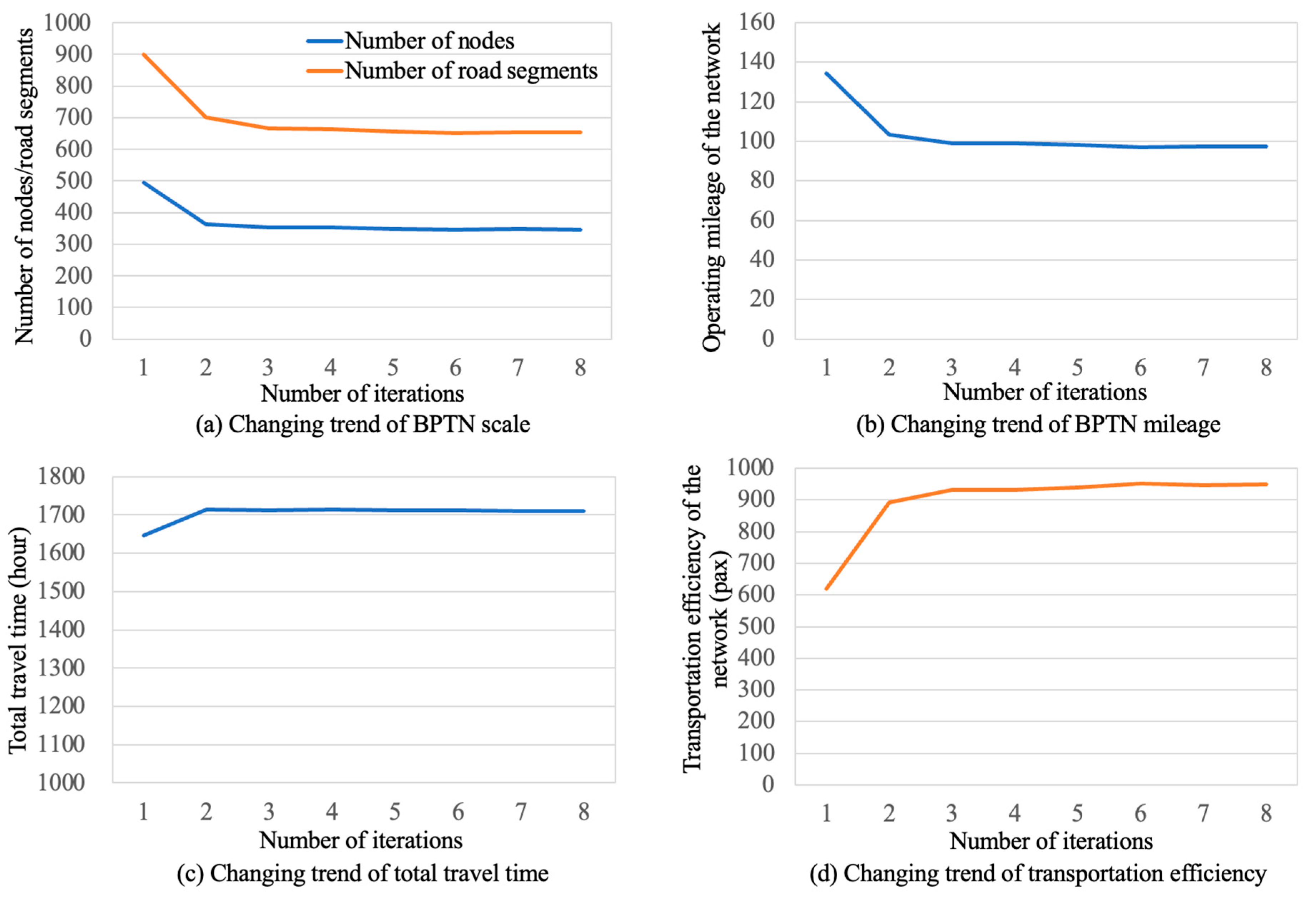
5.3. Analysis of the Computational Process

To demonstrate the efficacy and rationality of the algorithm, this subsection presents an analysis of the results obtained during the iterative process based on the example in Scenario 2. The initialized ETFD and BPTN at the beginning of the algorithm are illustrated in Figure 9a,b, respectively. Because all eligible road segments are assumed to provide associated transit services, the initial ETFD reflects passengers’ preferences regarding their expected transit routes for completing their trips. Therefore, the initial BPTN derived from this ETFD can optimize the overall expected travel time to a minimum. However, due to an excessively dispersed ETFD, the initial BPTN also becomes less efficient.

Based on the initial BPTN, the algorithm proceeds to the iteration phase. The algorithm converges to the final BPTN within eight iterations. The BPTNs obtained in each iteration are presented in Figure 10a–h, respectively, and the simplified topology graph by TGS is illustrated in Figure 10i. As can be seen, during this process, the selected paths connecting each OD pair gradually coupling with one another, efficiently reducing the scale of the BPTN and enhancing its transportation efficiency. Compared to the integrated transportation network with 4956 road segments and 2242 nodes, only three iterations are required for the number of segments and nodes in the BPTN to decrease to 667 and 353 respectively.

Moreover, the utilization of TGS enables further simplification of the final BPTN into a topological graph. As depicted in Figure 10i, the graph has only 66 edges and 45 nodes, where the blue nodes represent traffic zone centroids, and the red nodes indicate potential transfer nodes. Based on this simplified graph, the computational efficiency for subsequent optimization design of transit line deployment or other strategic and tactical decisions for transit systems can be significantly enhanced.

Figure 11 shows the changing trends in critical indicators for the BPTN over successive iterations. As shown in Figure 11a,b, the final scale of the BPTN has decreased by 27% and 7-fold compared to that of the first iteration and the integrated transportation network, respectively. The total mileage of the final BPTN is close to 100 km. This fulfills the minimum standard for network density in such a city with the planned area of 43.83 km². As illustrated in Figure 11c,d, there is a trade-off between reducing the overall travel time and enhancing the transportation efficiency during the optimization of the BPTN. However, there is only a marginal increase of 3.72% in the overall travel time during the second iteration, while witnessing a substantial improvement of 43.9% in transportation efficiency. Moreover, subsequent iterations continue to enhance transportation efficiency without significantly affecting the overall passenger travel time. In summary, the obtained BPTN effectively enhances transportation efficiency while ensuring an acceptable total travel time, thus demonstrating the efficacy and rationality of the proposed model and algorithm in maximizing BPTN utility.

5.4. BPTN Layouts Under Different Demand Structures

Based on the example in Scenario 2, we further examine the optimized BPTN layouts under two different demand structures, referred to as $Q_1$ and $Q_2$. $Q_1$ is the original demand structure used in Scenario 2. Moreover, the methods of ETFD analysis, assignment approaches, and parameter settings remain consistent with Scenario 2. The transit demand structures of $Q_1$ and $Q_2$ are presented in Figure 12a,b, respectively, while the corresponding results are depicted in Figure 12c,d. As can be seen, the optimized BPTN under demand structure $Q_2$ exhibits significant variations in the left and upper-left regions when compared to that of $Q_1$, thereby facilitating efficient routing for high-demand OD pairs. The number of segments and nodes in the final obtained BPTN under $Q_2$ decreases to 675 and 362, respectively. The scale of the BPTN is more than 7 times smaller than that of the original urban integrated transportation network. Moreover, the transportation efficiency is enhanced by 44.2% while only compromising 3.58% of the expected travel time. In other words, the proposed model and algorithm are capable of achieving BPTN layouts that align with diverse demand structures while effectively balancing travel time and transportation efficiency to enhance BPTN utility.

6. Conclusions

In this study, we investigate the BPTN layout planning problem for urban transit systems. The BPTN is represented as a set of paths connecting each OD pair, and its utility is formulated as the weighted sum of expected travel time and transportation efficiency associated with selected paths. To address the BPTN layout planning problem, we propose a non-linear integer programming model to maximize the utility of the BPTN. An ETFD analysis method combined with different assignment approaches is developed to evaluate the expected travel time and transportation efficiency of the BPTN under various types of transit systems. In addition, an objective–subjective integrated weighting approach is proposed to determine reasonable weight coefficients for travel time and transportation efficiency. The problem is solved by a heuristic solution framework with a TGS process, which further simplifies BPTN into a small-scale topological graph by identifying potential transfer nodes and merging road segments connecting centroids and transfer nodes.

Extensive numerical experiments are conducted based on a grid-shape integrated transportation network of a real city. The results show that our proposed model and algorithm are effective in obtaining desirable BPTN layouts for different types of transit systems, where travel time and transportation efficiency are well balanced to enhance BPTN utilities. The algorithm exhibits rapid convergence within limited iterations and the TGS process can significantly reduce the scale of the BPTN while maintaining critical characteristics and information. Moreover, the proposed model and algorithm are capable of obtaining BPTN layouts that align with different transit demand structures, providing valuable support for subsequent optimization design of transit line deployment or other strategic and tactical decisions for transit systems.

Future research work can be undertaken in several aspects. The solution framework in this study is designed to optimize the BPTN for one specific transit system at a time. Although we can fix the BPTN of one transit system and optimize the BPTN for another transit system to align with the fixed one, it is still an interesting direction to extend the framework to simultaneously consider multiple BPTN optimizations for diverse transit systems. Moreover, for simplification, transit demand in this study is assumed to be fixed. However, a higher-density BPTN has the potential to attract more passengers towards utilizing transit services. Future research endeavors could be undertaken to incorporate flexible transit demand in relation to the BPTN.

References

1. Ceder, A.; Wilson, N.H.M. Bus network design. Transp. Res. Part B Methodol. 1986, 20, 331–344. [Google Scholar] [CrossRef]
2. Baaj, M.H.; Mahmassani, H.S. An AI-based approach for transit route system planning and design. J. Adv. Transp. 1991, 25, 187–209. [Google Scholar] [CrossRef]
3. Arbex, R.O.; da Cunha, C.B. Efficient transit network design and frequencies setting multi-objective optimization by alternating objective genetic algorithm. Transp. Res. Part B Methodol. 2015, 81, 355–376. [Google Scholar] [CrossRef]
4. Liang, M.; Wang, W.; Dong, C.; Zhao, D. A cooperative coevolutionary optimization design of urban transit network and operating frequencies. Expert Syst. Appl. 2020, 160, 113736. [Google Scholar] [CrossRef]
5. Ahern, Z.; Paz, A.; Corry, P. Approximate multi-objective optimization for integrated bus route design and service frequency setting. Transp. Res. Part B Methodol. 2022, 155, 1–25. [Google Scholar] [CrossRef]
6. Cai, J.; Li, Z.; Long, S. Integrated Optimization of Route and Frequency for Rail Transit Feeder Buses under the Influence of Shared Motorcycles. Systems 2024, 12, 263. [Google Scholar] [CrossRef]
7. Li, S.; Liang, Q.; Han, K.; Wen, K. An SD-LV Calculation Model for the Scale of the Urban Rail Transit Network. Systems 2024, 12, 233. [Google Scholar] [CrossRef]
8. Mylonakou, M.; Chassiakos, A.; Karatzas, S.; Liappi, G. System dynamics analysis of the relationship between urban transportation and overall citizen satisfaction: A case study of Patras city, Greece. Systems 2023, 11, 112. [Google Scholar] [CrossRef]
9. Christofides, N. Graph Theory: An Algorithmic Approach (Computer Science and Applied Mathematics); Academic Press, Inc.: New York, NY, USA, 1975. [Google Scholar]
10. Garey, M.R.; Johnson, D.S. Computers and Intractability; W H Freeman: New York, NY, USA, 1979. [Google Scholar]
11. Golden, B.L.; Raghavan, S.; Wasil, E.A. (Eds.) The Vehicle Routing Problem: Latest Advances and New Challenges; Springer Science & Business Media: Berlin/Heidelberg, Germany, 2008; Volume 43. [Google Scholar]
12. Diestel, R. Graph Theory; Springer: Berlin/Heidelberg, Germany, 2005. [Google Scholar]
13. O’Kelly, M.E. The Location of Interacting Hub Facilities. Transp. Sci. 1986, 20, 92–106. [Google Scholar] [CrossRef]
14. Vuchic, V.R. Urban Transit: Operations, Planning, and Economics; John Wiley & Sons: Hoboken, NJ, USA, 2017. [Google Scholar]
15. Newell, G.F. Some issues relating to the optimal design of bus routes. Transp. Sci. 1979, 13, 20–35. [Google Scholar] [CrossRef]
16. Daganzo, C.F. Structure of competitive transit networks. Transp. Res. Part B Methodol. 2010, 44, 434–446. [Google Scholar] [CrossRef]
17. Thompson, G.L.; Matoff, T.G. Keeping Up with the Joneses: Radial vs. Multidestinational Transit in Decentralizing Regions. J. Am. Plan. Assoc. 2003, 69, 296–312. [Google Scholar] [CrossRef]
18. Nourbakhsh, S.M.; Ouyang, Y. A structured flexible transit system for low demand areas. Transp. Res. Part B Methodol. 2012, 46, 204–216. [Google Scholar] [CrossRef]
19. Chen, M.; Wu, F.; Yin, M.; Xu, J. Impact of road network topology on public transportation development. Wirel. Commun. Mob. Comput. 2021, 2021, 6209592. [Google Scholar] [CrossRef]
20. Zhang, M. Travel choice with no alternative: Can land use reduce automobile dependence? J. Plan. Educ. Res. 2006, 25, 311–326. [Google Scholar] [CrossRef]
21. Wong, R.C.P.; Szeto, W.Y.; Yang, L.; Li, Y.C.; Wong, S.C. Elderly users’ level of satisfaction with public transport services in a high-density and transit-oriented city. J. Transp. Health 2017, 7, 209–217. [Google Scholar] [CrossRef]
22. De Bona, A.A.; de Oliveira Rosa, M.; Fonseca, K.V.O.; Lüders, R. A reduced model for complex network analysis of public transportation systems. Phys. A Stat. Mech. Its Appl. 2021, 567, 125715. [Google Scholar] [CrossRef]
23. Bontorin, S.; Cencetti, G.; Gallotti, R.; Lepri, B.; De Domenico, M. Emergence of complex network topologies from flow-weighted optimization of network efficiency. Phys. Rev. X 2024, 14, 021050. [Google Scholar] [CrossRef]
24. Polimeni, A.; Vitetta, A. Network design and vehicle routing problems in road transport systems: Integrating models and algorithms. Transp. Eng. 2024, 16, 100247. [Google Scholar] [CrossRef]
25. Yujing, W.; Yi, D.; Fu, R.; Ruoxin, Z.; Pei, W.; Tian, D.; Qingyun, D. Analysing the spatial configuration of urban bus networks based on the geospatial network analysis method. Cities 2020, 96, 102406. [Google Scholar]
26. Shanmukhappa, T.; Ho, I.W.H.; Tse, C.K. Spatial analysis of bus transport networks using network theory. Phys. A Stat. Mech. Its Appl. 2018, 502, 295–314. [Google Scholar] [CrossRef]
27. Tian, Y.; Chen, H.; Xiao, D. The layout method for town public transit network based on TOD. In Proceedings of the International Conference on Transportation Engineering, Chengdu, China, 25–27 July 2009; pp. 1963–1968. [Google Scholar]
28. Badia, H.; Estrada, M.; Robusté, F. Competitive transit network design in cities with radial street patterns. Transp. Res. Part B Methodol. 2014, 59, 161–181. [Google Scholar] [CrossRef]
29. Fan, W.; Mei, Y.; Gu, W. Optimal design of intersecting bimodal transit networks in a grid city. Transp. Res. Part B Methodol. 2018, 111, 203–226. [Google Scholar] [CrossRef]
30. Manual, H.C. Highway Capacity Manual; The National Academies Press: Washington, DC, USA, 2000; Volume 2, p. 1. [Google Scholar]
31. Vuchic, V.R. Urban Transit Systems and Technology; John Wiley & Sons: Hoboken, NJ, USA, 2007. [Google Scholar]
32. Vince, A. A framework for the greedy algorithm. Discret. Appl. Math. 2002, 121, 247–260. [Google Scholar] [CrossRef]
33. Li, H.; Mao, B.; Bertini, R.L. Evaluating the impacts of bus facility design features on transit operations in Beijing, China: A simulation approach. In Proceedings of the 87th Annual Meeting of the Transportation Research Board, Washington, DC, USA, 13–17 January 2008. [Google Scholar]
34. Deng, T.; Nelson, J.D. Bus Rapid Transit implementation in Beijing: An evaluation of performance and impacts. Res. Transp. Econ. 2013, 39, 108–113. [Google Scholar] [CrossRef]
35. Spiess, H. Conical volume-delay functions. Transp. Sci. 1990, 24, 153–158. [Google Scholar] [CrossRef]
36. Bell, M.G. Alternatives to Dial’s logit assignment algorithm. Transp. Res. Part B Methodol. 1995, 29, 287–295. [Google Scholar] [CrossRef]
37. Wang, W.; Wang, J.; Zhao, D.; Jin, K. A Revised Logit Model for Stochastic Traffic Assignment with a Relatively Stable Dispersion Parameter. IEEE Intell. Transp. Syst. Mag. 2021, 14, 92–104. [Google Scholar] [CrossRef]
38. Dijkstra, E.W. A note on two problems in connexion with graphs. Numer. Math. 1959, 1, 269–271. [Google Scholar] [CrossRef]
39. Lee, C.K. A multiple-path routing strategy for vehicle route guidance systems. Transp. Res. Part C Emerg. Technol. 1994, 2, 185–195. [Google Scholar] [CrossRef]
40. Park, D. Multiple Path-Based Vehicle Routing in Dynamic and Stochastic Transportation Networks. Ph.D. Thesis, Texas A&M University, College Station, TX, USA, 1998. [Google Scholar]
41. Yen, J.Y. Finding the k shortest loopless paths in a network. Manag. Sci. 1971, 17, 712–716. [Google Scholar] [CrossRef]
42. Zhu, Y.; Tian, D.; Yan, F. Effectiveness of entropy weight method in decision-making. Math. Probl. Eng. 2020, 2020, 3564835. [Google Scholar] [CrossRef]
43. Cheng, Q.Y. Structure entropy weight method to confirm the weight of evaluating index. Syst. Eng. Theory Pract. 2010, 30, 1225–1228. [Google Scholar]
44. Chen, P. Effects of the entropy weight on TOPSIS. Expert Syst. Appl. 2021, 168, 114186. [Google Scholar] [CrossRef]
45. Kumar, R.; Singh, S.; Bilga, P.S.; Singh, J.; Singh, S.; Scutaru, M.-L.; Pruncu, C.I. Revealing the benefits of entropy weights method for multi-objective optimization in machining operations: A critical review. J. Mater. Res. Technol. 2021, 10, 1471–1492. [Google Scholar] [CrossRef]
Figure 1. Schematic of BPTN layout planning and TGS.
Systems 12 00550 g001
Figure 2. Schematic representation of different layout configurations of BPTN.
Systems 12 00550 g002
Figure 3. Flowchart for BPTN layout planning.
Systems 12 00550 g003
Figure 4. Flowchart of shortest-path incremental assignment.
Systems 12 00550 g004
Figure 5. Travel time and transportation efficiency of candidate paths for different OD pairs.
Systems 12 00550 g005
Figure 6. Subjective weights of travel time corresponding to different levels of demand under various values of ρ .
Systems 12 00550 g006
Figure 7. Illustration of integrated transportation network and demand structure.
Systems 12 00550 g007
Figure 8. BPTN layouts obtained in different calculation scenarios.
Systems 12 00550 g008
Figure 9. Initial ETFD and BPTN based on the example in Scenario 2.
Systems 12 00550 g009
Figure 10. Reproduced BPTN layouts through varying iterations and the simplified graph.
Systems 12 00550 g010
Figure 11. Changing trends in critical indicators for the BPTN over successive iterations.
Systems 12 00550 g011
Figure 12. BPTN layouts under different demand structures.
Systems 12 00550 g012