Development of a Forecasting Framework Based on Advanced Machine Learning Algorithms for Greenhouse Gas Emissions

Abstract

The reduction of greenhouse gas emissions, in order to effectively address the issue of climate change, has critical importance worldwide. To achieve this aim and implement the necessary strategies and policies, the projection of greenhouse gas emissions is essential. This paper presents a forecasting framework for greenhouse gas emissions based on advanced machine learning algorithms: multivariable linear regression, random forest, k-nearest neighbor, extreme gradient boosting, support vector, and multilayer perceptron regression algorithms. The algorithms employ several input variables associated with greenhouse gas emission outputs. In order to evaluate the applicability and performance of the developed framework, nationwide statistical data from Turkey are employed as a case study. The dataset of the case study includes six input variables and annual sectoral and total greenhouse gas emissions in CO₂ eq. as output variables. This paper provides a scenario-based approach for future forecasts of greenhouse gas emissions and a sector-based analysis of greenhouse gas emissions in the case country considering multiple input variables. The present study indicates that the stated machine learning algorithms can be successfully applied to the forecasting of greenhouse gas emissions.

1. Introduction

Global warming and climate change have emerged as some of the most significant environmental issues facing the global community in recent years. It is widely acknowledged that the primary driver of global climate change is the increase in greenhouse gas (GHG) emissions resulting from human activities. The GHG inventory consists of four primary GHGs: carbon dioxide, methane, nitrous oxide, and fluorinated gases. The total emissions are expressed in terms of carbon dioxide equivalent (CO₂ eq.) [1]. The United Nations Framework Convention on Climate Change (UNFCCC) entered into force in 1994. The ultimate objective of the UNFCCC is to stabilize GHG concentrations and prevent dangerous human interference with the climate system [2]. The Paris Agreement, which is one of the implementation instruments of the UNFCCC and sets the framework for the post-2020 climate change regime, was adopted at the 21st Conference of the Parties to the UNFCCC held in Paris in 2015. The principal goal of the Paris Agreement is to limit the global average temperature increase to well below 2 °C above pre-industrial levels and to pursue efforts to limit the temperature increase to 1.5 °C above pre-industrial levels [3,4]. In order to limit global warming to 1.5 °C, it is imperative that GHG emissions reach a peak before 2025 at the latest and subsequently decline by 43% by 2030. The Paris Agreement represents a significant milestone, as it represents the first instance where a binding agreement unites all nations in the collective effort of combating climate change and adapting to its effects [3]. Countries are adopting roadmaps for climate resilience, driven by increased environmental awareness following the Paris Agreement [5]. Turkey became a party to the UNFCCC in 2004. In 2021, Turkey ratified the Paris Agreement, thereby committing itself to achieving net zero emissions by 2053. This was announced on 27 September 2021 as part of the green development revolution [6]. As indicated in the GHG emission statistics released by the Turkish Statistics Institute (TurkStat), the level of GHG emissions in Turkey increased by 144.9% in 2022 when compared with emissions recorded in 1990. An examination of GHG emissions by sector reveals that, in 2022, the energy sector accounted for the largest proportion of the total GHG emissions at 71.8%. The energy sector was followed by the agricultural sector, which accounted for 12.8% of the total GHG emissions, the industrial processes and product use (IPPU) sector, which accounted for 12.5% of the total GHG emissions, and the waste sector, which accounted for 2.9% of the total GHG emissions [7]. It is of great importance for Turkey, as well as other countries, to establish strategies and policies aimed at reducing GHG emissions in order to achieve the desired targets. Considering the significance of GHG emissions for environmental issues, to contribute to the strategy and policy development of countries, many researchers have studied the forecasting of GHG emissions or CO₂ emissions. In order to forecast GHG or CO₂ emissions, a number of methods have been employed, including the use of statistical models, machine learning algorithms, metaheuristic algorithms, grey modelling, and deep learning algorithms, among others. A brief overview of some of these studies is presented.

Zhao et al. [8] employed a heterogeneity grey model to forecast carbon emissions in 30 provinces of China. The forecast results for the period from 2022 to 2030 were subjected to analysis on the basis of different scenarios of investment in environmental protection. Ayvaz et al. [9] developed a discrete grey modelling approach to forecast energy-related CO₂ emissions in Turkey, Europe, and Eurasia. Şahin [10] studied the problem of forecasting GHG emissions in Turkey with linear and nonlinear rolling metabolic grey models. Li et al. [11] developed an information priority generalized accumulative grey model. They applied the proposed model to the forecast of the GHG emissions of the Shanghai Corporate Organization. Ding et al. [12] developed a multivariate time-delay grey model. Renewable energy consumption, domestic credit to the private sector, gross capital formation, and labor forces were used as inputs to the developed model. The model was employed for the purpose of forecasting Chinese CO₂ emissions.

Hosseini et al. [13] used multiple linear regression and multiple polynomial regression models in order to build forecasting models of CO₂ emissions in Iran. They studied the population, CO₂ intensity, gross domestic product (GDP) per capita, the proportion of electricity generated from fossil fuels, and the per capita energy consumption as key drivers of CO₂ emissions, with these factors employed as predictors in regression analysis. Ho and Yu [1] studied GHG emission forecast in Hong Kong. They used a linear–log regression model with a principal component analysis to select the optimal predictors among potential predictors related to economics, social developments, energy use, waste production, and climatic conditions. Karakurt and Aydın [14] developed regression models to estimate CO₂ emissions arising from fossil fuels in BRICS (Brazil, the Russian Federation, India, China, and South Africa) and MINT (Mexico, Indonesia, Nigeria, and Turkey) countries. They used total population, urban population, and GDP per capita as variables in the proposed models. Özdemir et al. [15] aimed to forecast the total CO₂ emissions per capita as well as the per capita CO₂ emissions from energy industries, industrial processes, and the agricultural sector in Turkey. To achieve this, linear and logarithmic models were employed to analyze the potential impact of different scenarios.

Bakay and Ağbulut [16] proposed artificial neural networks (ANN), support vector machines (SVM), and deep learning algorithms for the forecasting of GHG emission types in Turkey. They used electricity production shares of energy resources as input parameters. Akyol and Uçar [17] aimed to estimate the GHG emissions of Turkey to determine their damage to the economy. They used linear sequential minimal optimization, multilayer perceptron, and regression algorithms. As independent variables, they employed energy production and consumption, GDP, and population. Ağbulut [18] studied the problem of forecasting transportation-related energy demands and CO₂ emissions in Turkey with deep learning, SVM, ANN, and linear and exponential regression models. Year, GDP, human population, and vehicle-kilometer were adopted as input parameters. AlKheder and Almusalam [19] proposed support vector machine, artificial neural networks, and deep learning algorithms to estimate the amount of CO₂ emissions from the power sector in Kuwait. Kumari and Singh [20] employed an autoregressive integrated moving average (ARIMA) model, a seasonal ARIMA model, a Holt–Winters model, a linear regression, a deep-learning-based long short-term memory (LSTM) model, and a random forest model to predict CO₂ emissions in India. Their study was restricted to the prediction of univariate CO₂ emissions. Giannelos et al. [21] utilized linear regression, ARIMA, shallow neural networks, and deep neural networks to predict CO₂ emissions in the building sector across a number of countries worldwide. Emami Javanmard et al. [22] developed a system that integrates multi-objective mathematical modelling with machine learning algorithms such as ARIMA, seasonal ARIMA, SVM, etc. Their objective was to estimate the energy demand and the CO₂ emissions in the Canadian transportation sector to examine the effect of energy resource type on the sector. Kayakuş et al. [5] aimed to develop a model consisting of environmental, social, and economic variables with the objective of predicting CO₂ emissions in Turkey. In order to accomplish this, machine learning techniques, including multiple linear regression, ANN, and support vector regression, were utilized. The outcomes were assessed in accordance with the specified targets of the European Union Green Deal.

Faruque et al. [23] used convolution neural networks (CNN), LSTM, CNN–LSTM, and dense neural networks to analyze the impact of energy consumption and GDP on CO₂ emissions in Bangladesh. Özcan et al. [24] employed deep learning models such as Prophet and LSTM to predict CO₂ in Turkey. Gloria and Höhn [25] developed CNN and image classification techniques to predict CO₂ eq. emissions for residential buildings. They used publicly available images of buildings and primary energy sources as inputs.

Sangeetha and Amudha [26] proposed multiple variable linear regression and particle swarm optimization algorithms to predict CO₂ emissions in India, considering coal, oil, natural gas, and primary energy consumption as input parameters. Bahmani et al. [27] designed Bat and Cuckoo optimization algorithms to predict global CO₂ emissions based on coal, natural gas, global oil, and primary energy consumption. Ene Yalçın [28] developed a particle swarm optimization algorithm to forecast the CO₂ emissions of Turkey by using primary energy consumption, GDP per capita, and population as input parameters. Arık et al. [29] utilized an artificial bee colony, a genetic algorithm, a simulated annealing algorithm, and hybrid versions of these algorithms to estimate the CO₂ emissions of Turkey. They used GDP, import, export, population, and construction permits as dependent variables.

For the forecasting of CO₂ emissions in Portugal from fossil fuel combustion and cement production, Belbute and Pereira [30] implemented an autoregressive fractionally integrated moving average approach. Yadav et al. [31] put forth a cross-sectional autoregressive distributed lag model to analyze the dynamics among robust governance, renewable energy investment, and green finance with respect to the mitigation of CO₂ emissions within the BRICS countries. Bennedsen et al. [32] developed a structural augmented dynamic factor model to estimate CO₂ emissions in the U.S. The researchers utilized variable selection techniques on a set of annual macroeconomic factors and concluded that CO₂ emissions were best explained by industrial production indices encompassing manufacturing and residential utilities.

As summarized above, a considerable number of researchers have made valuable contributions to the subject literature by employing a range of approaches. Among these approaches, machine learning algorithms have emerged as new and interesting alternative approaches. Moreover, efforts have been made to quantify GHG or CO₂ emissions in numerous countries, including Turkey. Considering the socioeconomic characteristics of different countries, as would be anticipated, the application of identical methodologies to disparate national contexts would yield disparate outcomes. Furthermore, the utilization of diverse methodologies and input variables for a given region can contribute to the projection of GHG or CO₂ emissions of the related regions. These findings demonstrate the continued necessity for the development of estimation models for GHG or CO₂ emissions.

This paper incorporates a number of algorithms to study the forecasting of GHG emissions, with an analysis of their performance based on a case study. A GHG emission forecasting framework is developed using machine learning algorithms: multivariable linear regression, random forest, k-nearest neighbor, extreme gradient boosting (XGBoost), support vector, and multilayer perceptron regression algorithms. Within the scope of the case study discussed in this paper, this approach aims to forecast the GHG emissions of Turkey through CO₂ eq. Year, population, GDP per capita, final energy consumption, renewable energy consumption, and industry production index are employed as input variables in the proposed algorithms to estimate GHG emissions in terms of CO₂ eq. While a number of studies have addressed the case of Turkey, this study develops a forecasting framework for greenhouse gas emissions based on advanced machine learning algorithms. The algorithms employ several input variables associated with GHG emission outputs. Furthermore, this study adopts a sector-based analysis, examining the contributions of the energy, IPPU, agricultural, and waste sectors in Turkey. To the best of the author’s knowledge, not much research has been conducted on sector-based GHG emission analysis considering multiple input variables with the presented algorithms. The rest of the paper is organized as follows. Section 2 presents the methodology and the adopted machine learning algorithms. Section 3 offers a description of the case data. The studied data characteristics, experimental results, discussion, and scenario-based future projections are provided in Section 4. Finally, the conclusions are presented in Section 5.

2. Materials and Methods

2.1. Machine Learning Algorithms

Machine learning is a method to enhance system performance through the implementation of computational processes that allow the system to learn from experience. Experience is represented by data, and the primary objective of machine learning is to design learning algorithms that construct models from the data. By inputting data into the learning algorithm, a model can be generated that is capable of making predictions regarding new observations [33]. Machine learning approaches have several application domains and have been widely studied in many areas such as healthcare, education, finance, mathematics, physics, and engineering [34,35,36,37,38,39,40].

Machine learning is generally divided into two main fields: supervised learning and unsupervised learning. In supervised learning, the machine learning algorithm is given labeled input examples [41]. Classification and regression are applications of this type of learning algorithm. Classification is described as the process of assigning one or more items to one of a number of predefined categories. Regression is defined as the process of estimating an output value on the basis of several influencing factors. In the context of classification, the resulting output value is discrete; conversely, in the context of regression, the output value is continuous [42]. The process of unsupervised learning involves the creation of models based on the analysis of similarities between unlabeled input data. Clustering is a typical application area in unsupervised learning [41].

2.1.1. Multiple Linear Regression

Linear regression is a method that predicts the value of one variable in relation to another. The variable that is to be estimated is referred to as the dependent variable, while the variable utilized to estimate the value of the other variable is known as the independent variable [5]. In multiple linear regressions, multiple independent variables are employed. The multiple linear regression formula is given in Equation (1).

$$y_i=({\beta }_0+{\beta }_1{X}_{1i}+{\beta }_2{X}_{2i}+{\beta }_3{X}_{3i}+\cdots +{\beta }_n{X}_{ni})+{\epsilon }_i$$

(1)

where y_i is the dependent variable to be predicted, ${\beta }_1$ is the coefficient of the first independent variable X_1i, ${\beta }_2$ is the coefficient of the second independent variable X_2i, ${\beta }_n$ is the coefficient of the nth independent variable X_ni. The term ${\epsilon }_i$ represents the error [43]. The basic linear model, despite its relatively simple form and its ease of modelling, encapsulates a number of fundamental ideas in the field of machine learning [33].

2.1.2. Random Forest Regression

Classification and regression type problems can be solved with random forest models, which are examples of a supervised technique [20]. This algorithm is capable of detecting nonlinear relationships among dependent and independent variables. A decision tree represents if-then rules in a hierarchical structure. The final structure comprises two types of elements: nodes (decision rules) and leaves (decisions). Prior to the construction of a tree, it is essential to determine the minimum number of samples required for node splitting and the maximum depth of the tree [44]. The random forest technique employs the ensemble learning approach to regression, wherein a multitude of decision trees are randomly fitted and subsequently averaged to yield the forest’s forecast [45]. Random forest frequently demonstrates a remarkably robust performance in practical applications, earning recognition as a paragon of contemporary ensemble learning methodologies [33].

2.1.3. K-Nearest Neighbor Regression

K-nearest neighbor (kNN) is one of the most widely employed classification algorithms. kNN is one of the supervised learning algorithms, and it is also used for regression and time series prediction [46]. The kNN regression model is based on the determination of the distance between a new observation point and all the observations in the training dataset. The Euclidean distance is the most preferred distance metric. Following the calculation of the distances, the kNN algorithm identifies the k neighbors with the shortest distances. Subsequently, the predicted value of the new observation $\widehat{y}$ is derived as the average (or median) of the target variable values of the k nearest neighbors, as represented in Equation (2). Simplicity is one of the strengths of kNN regression and the choice of a value for k has critical importance [47,48].

$$\widehat{y}={\displaystyle \frac{1}{k}}{\sum }_{i=1}^k{y}_i\left(x\right)$$

(2)

2.1.4. XGBoost Regression

XGBoost is an ensemble machine learning algorithm designed for regression and classification tasks. The method facilitates computational efficiency and enhanced model flexibility in supervised learning. XGBoost integrates the predictive capacity of numerous learners into a unified model through a process of iterative consolidation. Decision trees are employed as base learners. At each iteration, the calculated error is utilized to refine the preceding predictor (learner), while the alteration in model performance is assessed through the utilization of the objective function [49]. The objective function is the sum of loss and regularization functions, as shown in Equation (3) [50]:

$$Objective function={\sum }_{i=1}^{n}l\left(y_i,{\widehat{y}}_i\right)+{\sum }_{j=1}^m\Omega {(f}_j)$$

(3)

where $l\left(y_i,\widehat{y_i}\right)$ is the loss function and $\Omega {(f}_j)$ is the regularization function added to the objective function to control the complexity of the model and avoid overfitting. The XGBoost algorithm is designed to construct classification and regression trees one after the other. The training of each tree is based on the errors encountered in the previous tree. This process leads to the creation of a new tree with a reduced error rate, which, in turn, enables the generation of a prediction [51].

2.1.5. Support Vector Regression

Support vector machine is a supervised learning method utilized for classification and regression problems. Support vector regression is the adaptation of support vector machine for regression. In comparison to alternative conventional learning techniques, this method demonstrates a superior performance and the ability to address nonlinear problems [5]. ${\left\{x_i,y_i\right\}}_{i=1}^N$ is described as a dataset where N represents the quantity of training instances and the terms x_i and y_i denote the input and output variables, respectively. A nonlinear function $\varphi \left(x\right)$ is used to transform the input data from low dimensional to high dimensional space. It aims to identify f(x), which is a function that approximates all instances. Subsequently, the regression equation is calculated according to Equation (4) [52]:

$$f\left(x\right)=w\cdot \varphi \left(x\right)+b$$

(4)

where w indicates the weight and b indicates the bias. Next, the regression equation is expressed as an optimization problem, given in Equations (5) and (6) [52]:

$$\mathit{min}{\displaystyle \frac{1}{2}}{‖w‖}^2+C{\sum }_{i=1}^N({\delta }_i+{\delta }_i^{\ast })$$

(5)

$$s.t. \left\{\begin{array}{c}{y}_i-w\cdot \varphi \left(x\right)-b\le \epsilon +{\delta }_i\\ w\cdot \varphi \left(x\right)+b-y_i\le \epsilon +{\delta }_i^{\ast }\\ {\delta }_i,{\delta }_i^{\ast }\ge 0, i=\mathrm{1,2},\dots ,N\end{array}\right.$$

(6)

where C is the regularization parameter that identifes the trade-off between the flatness of f(x) and the $\epsilon$ loss function and ${\delta }_i,{\delta }_i^{\ast }$ are slack variables [45]. The optimization problem is then reformulated as a dual optimization problem using the Lagrange multiplier method, thereby enabling the nonlinear function to be obtained as in Equation (7):

$$f\left(x\right)={\sum }_{i=1}^N{(\alpha }_i-{\alpha }_i^{\ast }\left)K\right(x_i,x_j)+b$$

(7)

where ${\alpha }_i,{\alpha }_i^{\ast }$ are Lagrangian multipliers and $K(x_i,x_j)$ is the kernel function [45]. The choice of kernel function determines the learning performance of the method. Commonly utilized kernel functions include the linear, polynomial, and radial basis function [52].

2.1.6. Multilayer Perceptron Regression

Multilayer perceptron is a type of artificial neural network that can be applied to both classification and regression problems [53]. Typically, multilayer perceptrons have an input layer, one or more hidden layers, and an output layer [54]. For a multilayer perceptron model comprising a single hidden layer and a single output, the formula of the output can be expressed as in Equation (8) [55]:

$$\widehat{y}={\xi }_2\left({\sum }_{i=1}^m{w}_i^{\left(2\right)}{\xi }_1\left({\sum }_{j=1}^n{x}_j{w}_j^{\left(1\right)}+b^{\left(1\right)}\right)+b^{\left(2\right)}\right)$$

(8)

In the equation given above, $\widehat{y}$ refers to the predicted vector, while the quantity of data vectors in the complete dataset and the quantity of input variables are displayed as m and n, respectively. The term x_j represents the feature vector j. The term w⁽²⁾ denotes the weights between the hidden and the output layer, while w⁽¹⁾ denotes the weights between the input and the hidden layer. The activation function of the output layer is shown as ${\xi }_2$, while the activation function of the hidden layer is shown as ${\xi }_1$. The terms b⁽²⁾ and b⁽¹⁾ represent the bias vectors for the output and hidden layer, respectively [55]. The size of the hidden layers, the activation functions, and the solver function are among the hyperparameters of this algorithm [48]. The generally employed activation functions, which are ReLU, sigmoid, and tanh functions, are presented in Equations (9)–(11) [54].

$$ReLU=\max \left(0,x\right)$$

(9)

$$sigmoid \left(x\right)={\displaystyle \frac{1}{(1+e^{-x})}}$$

(10)

$$\mathit{tanh} \left(x\right)={\displaystyle \frac{e^x-e^{-x}}{e^x+e^{-x}}}$$

(11)

2.2. Performance Evaluation

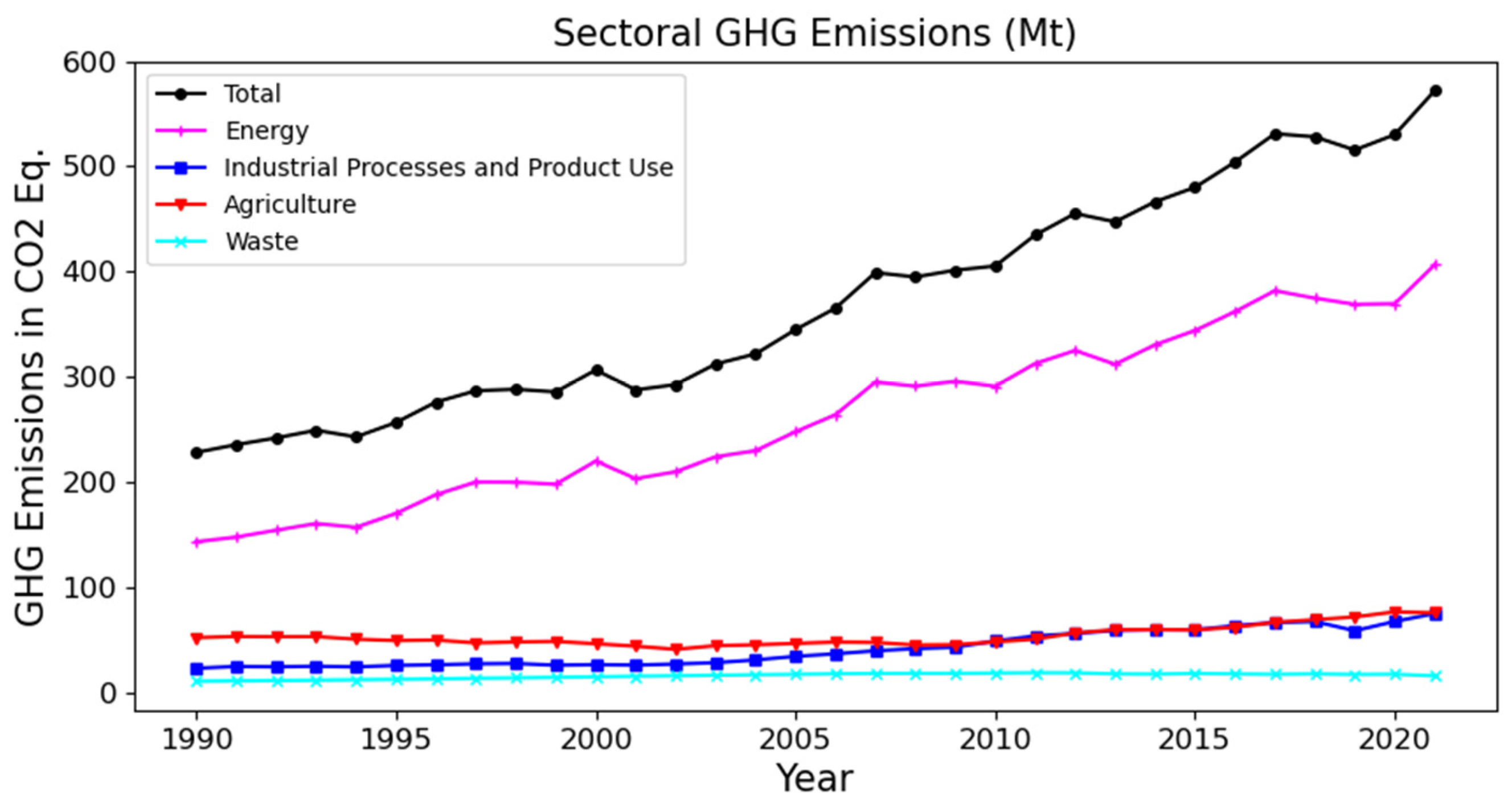
In order to validate the efficacy of the forecasting models, researchers have employed a range of performance metrics, as outlined in the existing forecasting literature [56]. To evaluate the performance of the algorithms, the mean square error (MSE), mean absolute error (MAE), root mean square error (RMSE), mean absolute percentage error (MAPE), and the determination coefficient (R²) measures, given in Equations (12)–(16), are used in this paper. In the following equations, $y_i$ represents the observed value, ${\widehat{y}}_i$ represents the predicted value, and n shows the total number of data points.

$$MSE={\displaystyle \frac{1}{n}}{\sum }_{i=1}^n{(y_i-{\widehat{y}}_i)}^2$$

(12)

$$MAE={\displaystyle \frac{{\sum }_{i=1}^n\left|y_i-{\widehat{y}}_i\right|}{n}}$$

(13)

$$RMSE=\sqrt{{\displaystyle \frac{1}{n}}{\sum }_{i=1}^n(y_i-{\widehat{y}}_i)}$$

(14)

$$MAPE={\displaystyle \frac{1}{n}}{\sum }_{i=1}^n\left|{\displaystyle \frac{y_i-{\widehat{y}}_i}{y_i}}\right|\times 100$$

(15)

$$R^2=1-{\displaystyle \frac{{\sum }_{i=1}^n{(y_i-{\widehat{y}}_i)}^2}{{\sum }_{i=1}^n{(y_i-{\overline{y}}_i)}^2}}$$

(16)

While the MSE quantifies the average squared difference between the observed and predicted values yielded by a model, the MAE computes the mean of the absolute differences between the observed and predicted values [51]. The RMSE is the square root of the MSE. The MAPE measures the error in a prediction model as a percentage [17]. For MSE, MAE, RMSE, and MAPE, smaller values, values close to 0, reflect a high prediction performance. The R² is a metric that shows how a model fits the observed data. R² takes values from 0 to 1, and higher values of R², values close to 1, indicate high accuracy for a forecasting model [5]. The forecasting methodology proposed in this paper is summarized in Figure 1.

3. Data Description

The required data for the case study of Turkey were collected from different sources. Data on the total GHG emissions of Turkey in CO₂ eq. from the year 1990 to 2021 were obtained from TurkStat and used as output data. Additionally, for the sectoral analysis, the total GHG emissions in CO₂ eq. by sector were utilized for output data and collected from TurkStat. The total GHG emissions in CO₂ eq. of Turkey from the year 1990 to 2021 are shown in Figure 2 as million tonnes (Mt) by sector.

Year, population, GDP per capita, final energy consumption, renewable energy consumption, and industry production index were employed as input variables. The data on population and GDP per capita from the year 1990 to 2021 were collected from the World Bank. The data on final energy consumption and renewable energy consumption from the year 1990 to 2021 were collected from the International Energy Agency. Finally, the industry production index data from the year 1990 to 2021 were obtained from TurkStat.

Table 1. Descriptive statistics of the dataset.

Dataset	Average	Min	Max	Standard Deviation
Year	2005.5	1990	2021	9.380
Population	69,201,210	54,324,140	84,147,320	8,955,316
GDP per capita (TRY)	17,109.515	7.24	86,231.420	20,811.961
Final energy consumption (PJ)	2972.531	1691	4820	937.311
Renewable energy consumption (PJ)	274.500	217	322	37.053
Industry production index variables (2021 = 100)	49.322	23.280	100	22.772
GHG emissions in CO2 eq. (Mt)	371.425	228	572	106.297
GHG emissions in CO2 eq. for the energy sector (Mt)	261.695	143.147	406.472	80.735
GHG emissions in CO2 eq. for the IPPU sector (Mt)	41.043	22.691	74.715	16.953
GHG emissions in CO2 eq. for the agricultural sector (Mt)	53.277	40.708	76.437	9.599
GHG emissions in CO2 eq. for the waste sector (Mt)	15.407	10.315	18.434	2.562

presents descriptive statistics of the dataset.

4. Results and Discussion

In this paper, six different machine learning methods were applied to the case dataset of GHG emissions in Turkey, namely multivariable linear regression, random forest, kNN, XGBoost, support vector, and multilayer perceptron regression algorithms. The algorithms under consideration in the present study were developed using Python. The dataset included six input variables and annual sectoral and total GHG emissions in CO₂ eq. as output variables. The input parameters included year, population, GDP per capita, final energy consumption, renewable energy consumption, and industry production index. In the data preprocessing phase, in order to understand the relationship among the input and output variables, a correlation analysis using the Pearson correlation method was performed. Upon evaluation of the obtained correlation coefficients, it can be observed that there was a very strong relationship between each input variable and the output variable total GHG emissions in CO₂ eq. Similar results were obtained with respect to the relationship between each input variable and the output variables GHG emissions in CO₂ eq. for the energy and IPPU sectors. With respect to the output variable GHG emissions in CO₂ eq. for the agricultural sector, strong and very strong relationships were detected with the input variables. In relation to the output variable GHG emissions in CO₂ eq. for the waste sector, a moderate relationship was identified with the GDP per capita input variable, while strong and very strong relationships were detected with the remaining input variables. Note that, during the data preprocessing, normalization was conducted for the support vector and multilayer perceptron regression algorithms.

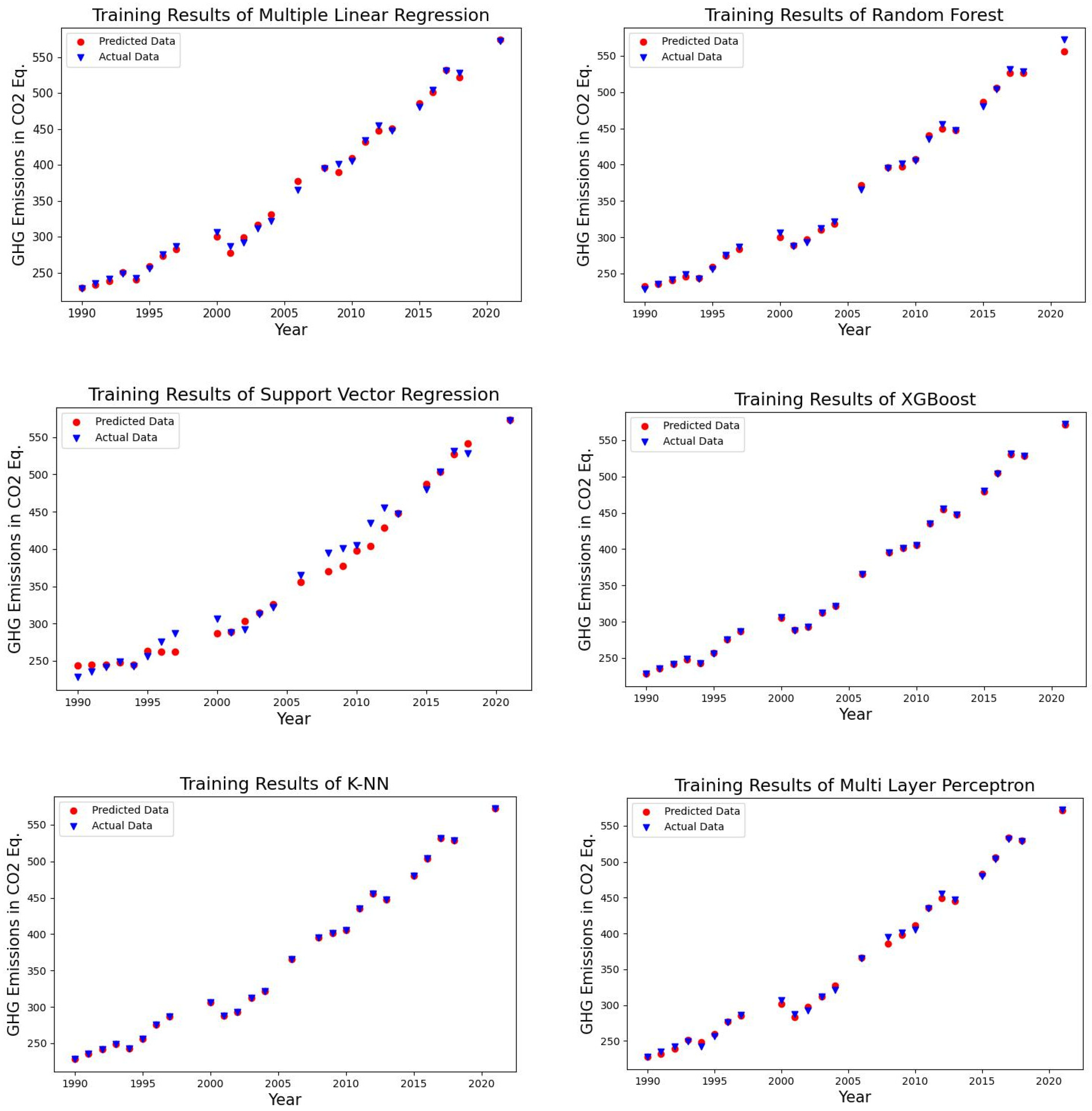
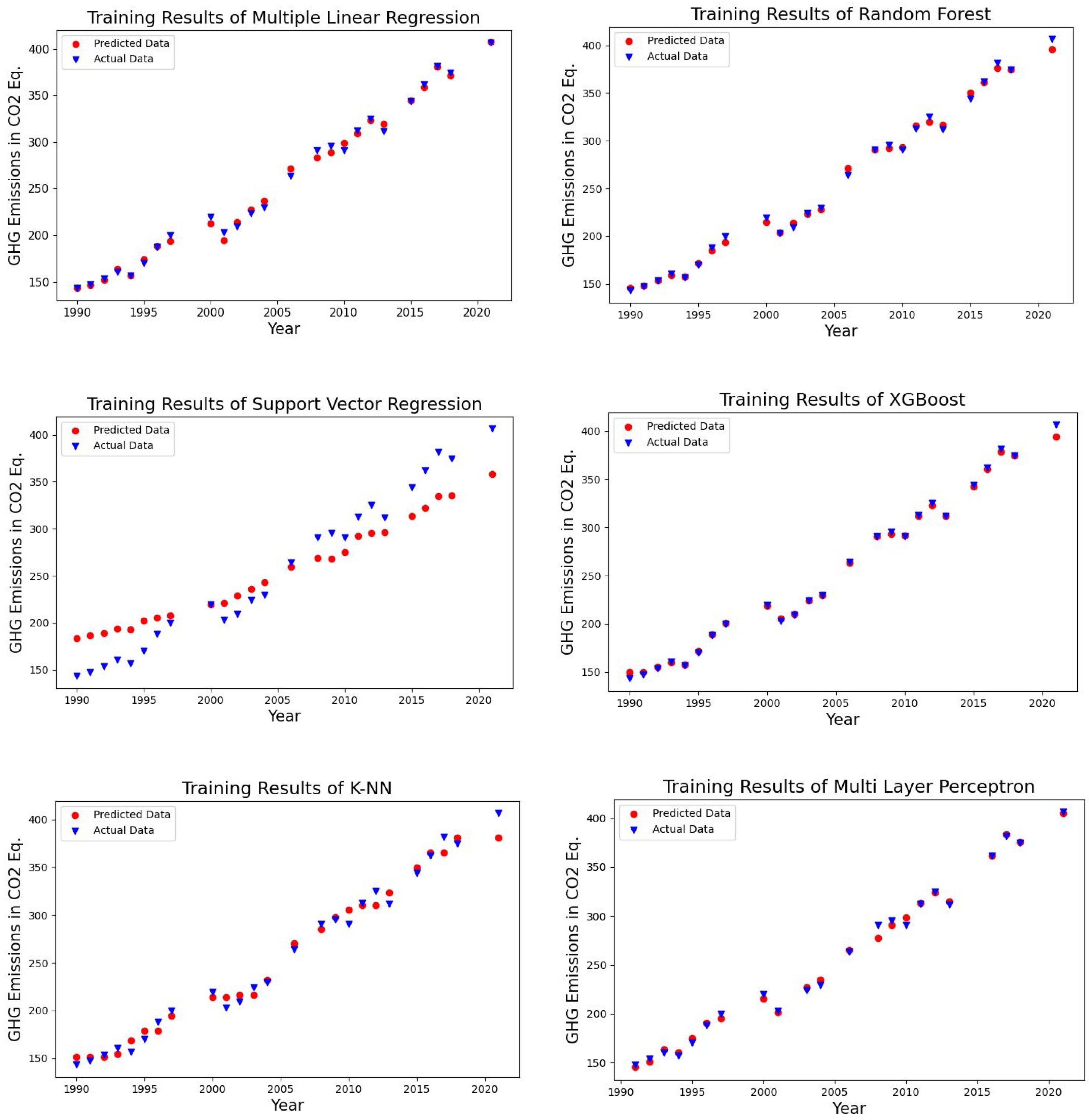
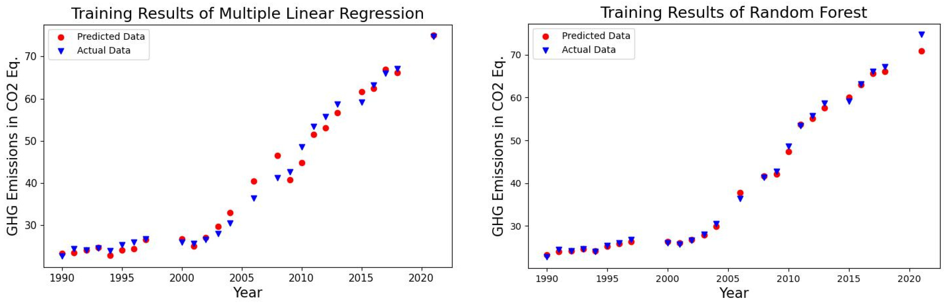
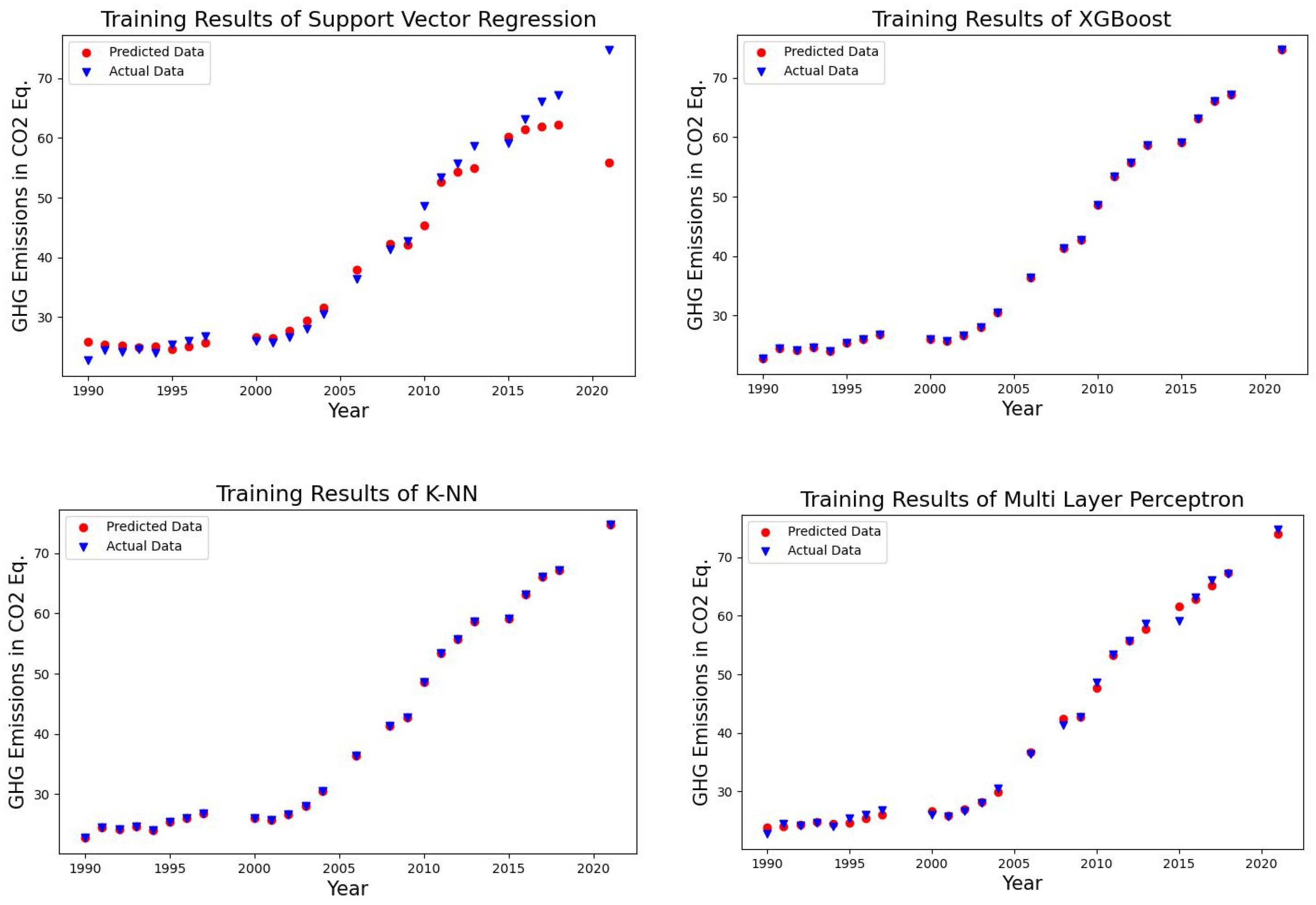
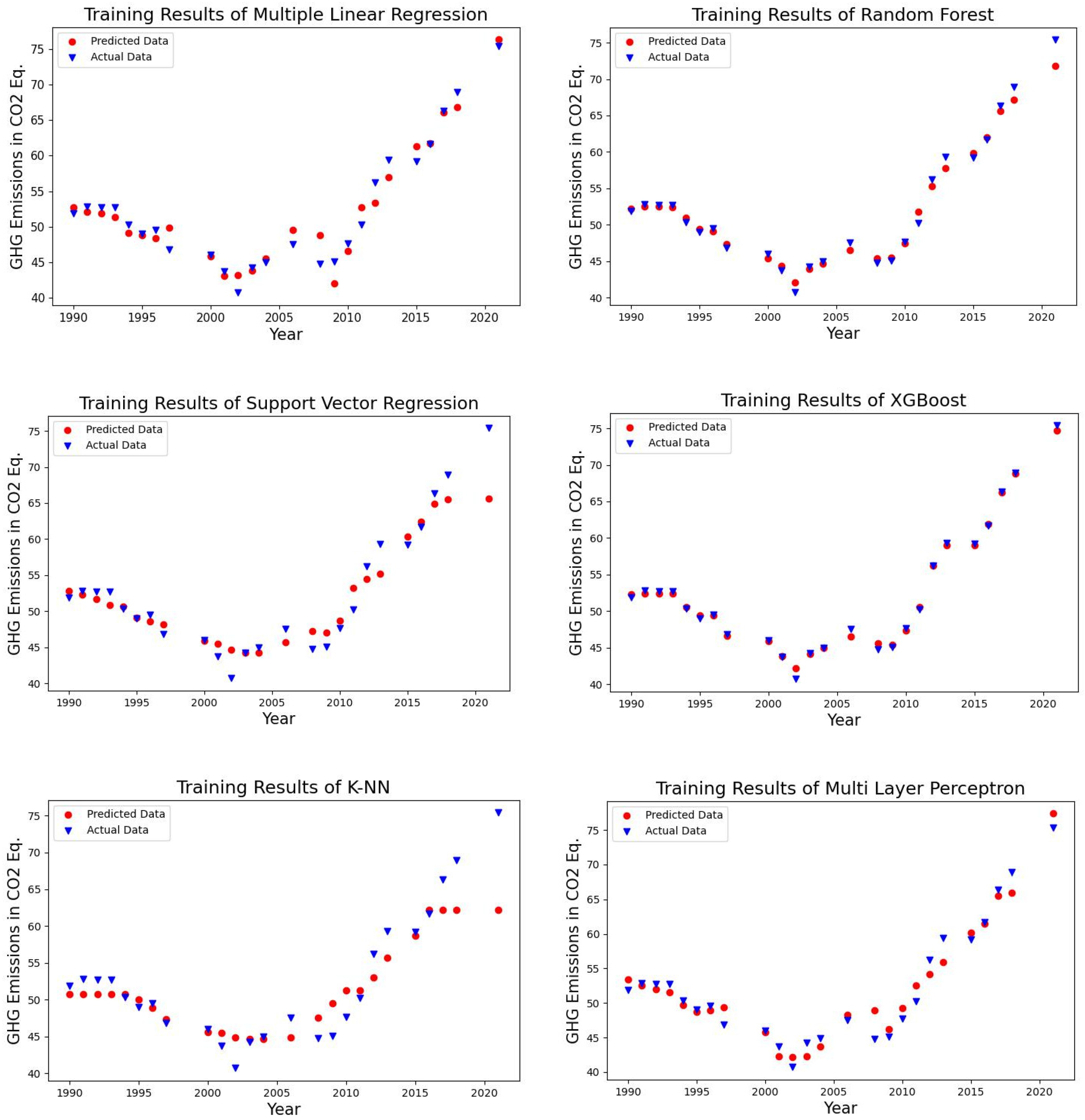
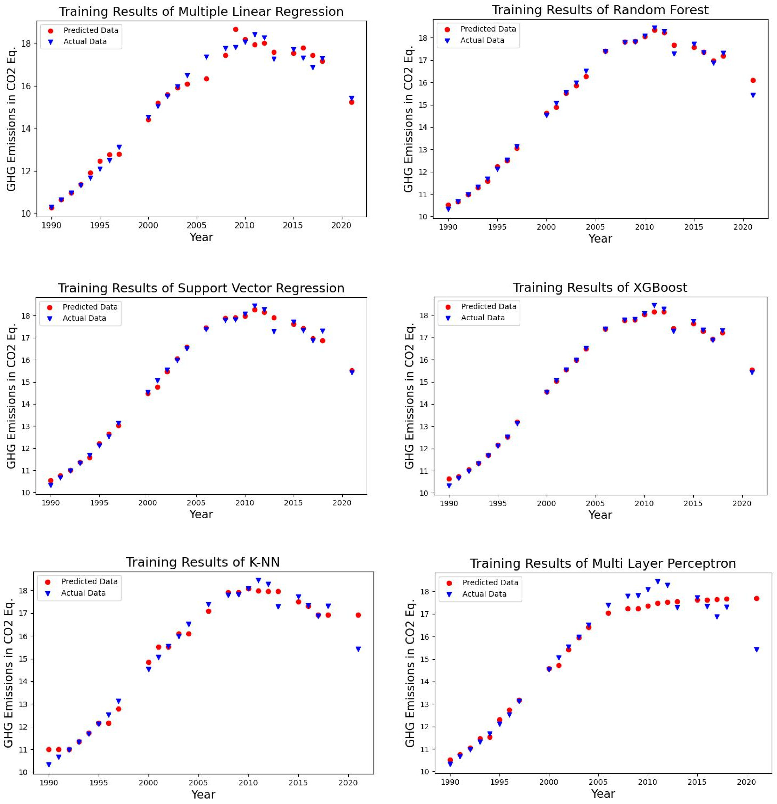
4.1. Forecasting Results of the Algorithms

The studied dataset was divided into two parts for training and testing purposes. In all employed machine learning models, 80% of the dataset was used for training, and 20% of the dataset was used for testing. To tune the parameters of the employed models, the grid search technique was applied. Figure 3 shows the training results of the algorithms for the total GHG emissions in CO₂ eq.

Table 2. Performance results of the algorithms for the test data on the total GHG emissions in CO₂ eq.

Algorithms	MSE	MAE	RMSE	MAPE %	R2
Multiple linear regression	32.279	5.155	5.681	1.391	0.996
Random forest regression	69.716	6.955	8.350	1.665	0.992
Support vector regression	771.655	25.593	27.779	6.373	0.915
XGBoost regression	159.023	9.301	12.610	2.468	0.982
kNN regression	234.900	11.657	15.326	2.715	0.974
Multilayer perceptron regression	245.362	12.263	15.664	2.677	0.973

presents a comparison of the performance results of the algorithms in relation to the test data under the consideration of this paper for the total GHG emissions in CO₂ eq. output.

According to the performance results of the six machine learning algorithms summarized with respect to the related metrics, given in Table 2, all algorithms attained satisfying results in terms of the R² performance measure. The R² performance measure ranged between 0.915 and 0.996. To ensure the accuracy of a forecast, Lewis [57] suggested reference values in terms of the MAPE performance measure. According to this classification, when the range of MAPE is ≤ 10%, forecasting accuracy is categorized as “high”. When the range of MAPE is 10–20%, forecasting accuracy is categorized as “good”. When the range of MAPE is 20–50%, forecasting accuracy is categorized as “feasible”. When the range of MAPE is ≥50%, forecasting accuracy is categorized as “low”. By considering these reference values, it can be observed that the forecasting accuracy was high for all algorithms. Moreover, the multiple linear regression algorithm obtained the best results in relation to the MSE, MAE, RMSE, MAPE, and R² performance measures with respect to the total GHG emissions in CO₂ eq. in Turkey. The random forest regression algorithm was found to be the second-best algorithm, following the multiple linear regression algorithm in all performance measures.

In order to obtain sector-based findings, the sectoral GHG emissions in CO₂ eq. outputs were subjected to further analysis. Turkey maintains sector-specific GHG emission statistics for the energy, IPPU, agricultural, and waste sectors. Therefore, the algorithm comparisons were made for these sectors. The training results of the employed algorithms for the sectoral GHG emissions in CO₂ eq. are presented in Figure 4, Figure 5, Figure 6 and Figure 7.

Table 3. Performance results of the algorithms in relation to the test data on the GHG emissions in CO₂ eq. from the energy sector.

Algorithms	MSE	MAE	RMSE	MAPE %	R2
Multiple linear regression	63.977	6.508	7.999	2.239	0.986
Random forest regression	67.510	6.704	8.216	2.252	0.985
Support vector regression	445.461	18.568	21.106	6.159	0.904
XGBoost regression	99.512	7.927	9.976	2.745	0.979
kNN regression	152.716	10.267	12.358	3.574	0.967
Multilayer perceptron regression	129.589	10.059	11.384	3.401	0.972

shows the performance results of the algorithms in relation to the test data on GHG emissions in CO₂ eq. for the energy sector in Turkey. The performance results of the algorithms in relation to the test data on GHG emissions in CO₂ eq. for the IPPU, agricultural, and waste sectors in Turkey are presented in

Table 4. Performance results of the algorithms in relation to the test data on the GHG emissions in CO₂ eq. from the IPPU sector.

Algorithms	MSE	MAE	RMSE	MAPE %	R2
Multiple linear regression	13.611	2.889	3.689	6.623	0.945
Random forest regression	11.364	2.120	3.371	4.485	0.954
Support vector regression	8.264	2.030	2.875	3.862	0.966
XGBoost regression	13.270	2.391	3.643	5.298	0.946
kNN regression	24.894	2.877	4.989	5.208	0.899
Multilayer perceptron regression	17.755	2.657	4.214	5.188	0.928

,

Table 5. Performance results of the algorithms in relation to the test data on the GHG emissions in CO₂ eq. from the agricultural sector.

Algorithms	MSE	MAE	RMSE	MAPE %	R2
Multiple linear regression	29.191	3.882	5.403	6.175	0.789
Random forest regression	10.299	2.216	3.209	3.426	0.926
Support vector regression	18.638	2.814	4.317	4.184	0.865
XGBoost regression	10.781	2.370	3.284	3.709	0.922
kNN regression	43.440	4.470	6.591	6.796	0.686
Multilayer perceptron regression	18.355	3.246	4.284	5.103	0.868

, and

Table 6. Performance results of the algorithms in relation to the test data on the GHG emissions in CO₂ eq. from the waste sector.

Algorithms	MSE	MAE	RMSE	MAPE %	R2
Multiple linear regression	0.392	0.586	0.626	3.567	0.831
Random forest regression	0.086	0.238	0.293	1.529	0.963
Support vector regression	0.166	0.299	0.407	1.850	0.928
XGBoost regression	0.203	0.321	0.451	2.159	0.912
kNN regression	0.090	0.209	0.300	1.251	0.961
Multilayer perceptron regression	0.264	0.439	0.513	2.652	0.886

, respectively.

When the results for the GHG emissions of the energy sector in CO₂ eq. were analyzed, a similarity to the total GHG emissions emerged. All algorithms attained convincing results in terms of the R² performance measure, since the R² performance measure ranged between 0.904 and 0.986. Based on the MAPE performance measure, the forecasting accuracy of all six algorithms was high. The multiple linear regression algorithm achieved the best results in terms of MSE, MAE, RMSE, MAPE, and R² performance measures.

Based on the performance results in relation to the GHG emissions from the IPPU sector in CO₂ eq., the forecasting accuracy of all algorithms was high in terms of the MAPE performance measure. The support vector regression algorithm delivered the best performance across all performance measures. The random forest regression algorithm emerged as the second-best algorithm.

A detailed examination of the GHG emissions in CO₂ eq. from the agricultural sector revealed the following results. The random forest regression algorithm achieved the best results in terms of MAPE, R², MSE, MAE, and RMSE. The XGBoost regression algorithm emerged as the second-best algorithm across all performance measures. Although the MAPE results of the kNN regression algorithm indicated a high forecasting accuracy, the R² value of this algorithm was only 0.686.

Performance results in relation to the GHG emissions from the waste sector in CO₂ eq. show that the forecasting accuracy of all algorithms was high with respect to the MAPE performance measure. The R² values ranged between 0.831 and 0.963. While the random forest algorithm obtained the highest R² value, the kNN regression algorithm achieved the best results in terms of the MAPE performance measure, followed by the random forest algorithm.

To sum up, the obtained results show that all employed machine learning algorithms attained a high forecasting accuracy in relation to both the total GHG emissions in Turkey in CO₂ eq. and the sectoral GHG emissions in Türkiye in CO₂ eq. While each algorithm can be utilized for forecasting purposes, the most suitable algorithm for a given task can be selected based on the desired forecast accuracy.

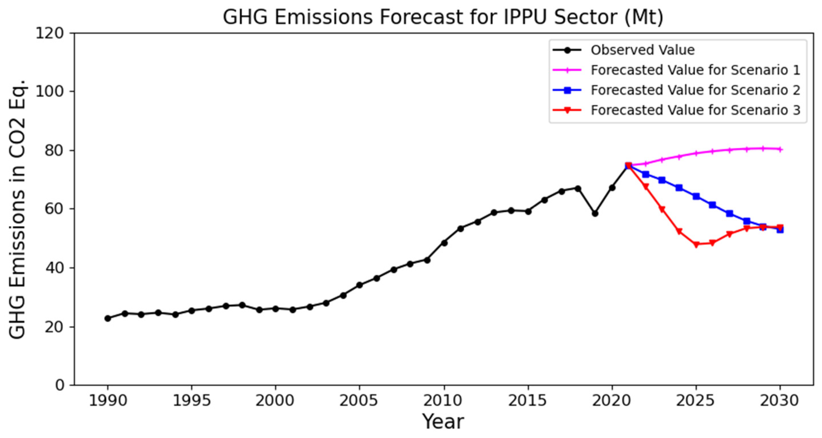
4.2. Scenario Analysis

Since future values of the input variables are uncertain, a scenario-based approach can be implemented to make predictions for future periods. Under the scope of this paper, three scenarios were defined. Under scenario 1, each of the input variables was made to behave similarly to their past trends, in other words, they exhibited an increasing trend. Future values of the input variables were, therefore, estimated using an exponential smoothing method based on their past values. Under scenario 2, while the final energy consumption input variable was made to follow a stable trend, the renewable energy consumption input variable was made to exhibit a slightly increasing trend, which was set to 10%. The remaining input variables were set to behave according to their past trends and were obtained by using an exponential smoothing method. Finally, under scenario 3, the final energy consumption input variable was made to experience a 5% decrease, the renewable energy consumption input variable was made to experience an increasing trend of 20%, and the remaining variables were set not to demonstrate a discernible pattern of change, whether one of decline or increase. Figure 8 presents the total GHG emissions forecast results in Turkey for the defined scenarios until 2030, obtained by using the multiple linear regression algorithm.

As illustrated in Figure 8, the future forecast results indicate that, due to the inclusion of input variables showing an increasing trend under scenario 1, the total GHG emissions in CO₂ eq. are projected to increase until 2030 according to scenario 1. Under scenario 2, the increase in GHG emissions is also projected to persist, but at a decelerating rate. It can be observed from Figure 8 that, under scenario 3, the total GHG emissions begin to exhibit a decline. The forecast results of the GHG emissions in CO₂ eq. from the energy, IPPU, agricultural, and waste sectors in Turkey until 2030 are presented in Figure 9, Figure 10, Figure 11, and Figure 12, respectively. While the GHG emission forecast results from the energy sector under the defined scenarios until 2030 were obtained by using the multiple linear regression algorithm, the forecast results for the IPPU sector were obtained through the support vector regression algorithm. Forecast results for the agricultural and waste sectors were obtained through the random forest regression algorithm.

Based on the GHG emission forecast results for the energy sector, shown in Figure 9, it can be concluded that, as in the case of the total GHG emission forecast results, GHG emissions from the energy sector are projected to continue to increase until 2030 under scenario 1. A consistent trend is projected under scenario 2. Under scenario 3, a slightly decreasing trend is projected for the emissions from the energy sector. It should be noted that the energy sector accounts for the largest share of the total GHG emissions in Turkey.

With respect to the GHG emission forecast results in relation to the IPPU sector, presented in Figure 10, a slowly increasing trend can be observed under scenario 1. While a noticeable decrease under scenario 2 can be observed in terms of GHG emissions, a strongly decreasing trend, followed by a slight increase in GHG emissions, can be observed under scenario 3 until 2030.

Upon analysis of the GHG emission forecast results for the agricultural sector, shown in Figure 11, it can be concluded that, based on the fitted model, while under scenario 3 there is a noticeable decrease, under scenarios 1 and 2 the GHG emission forecast appears in the form of a consistent trend.

Finally, as illustrated in Figure 12, it can be stated that, based on the trend of the past values and the fitted model, the GHG emission forecast results for the waste sector demonstrate a consistent trend under all scenarios until 2030, although, in relation to scenarios 2 and 3, consistency can be observed after a slight downward trend.

The forecasting results in relation to the total and sectoral GHG emissions in CO₂ eq. were compared with the actual most recent data for validation. Figure 13 presents a comparison of the forecasting results with the actual data for the year 2022. It can be observed that the scenario-based forecasting produced results that are in close approximation to the actual values.

The sensitivity of the total GHG emission in CO₂ eq. output to changes in the final energy consumption, GDP per capita, renewable energy consumption, and industry production index input variables was evaluated by adding and removing 50%, 35%, 20%, and 10% to the specified input variables. Figure 14 presents the results of the sensitivity analysis.

The results of the sensitivity analysis demonstrate that the total GHG emissions of Turkey are more affected by changes in the input variables of final energy consumption and industry production index, with the final energy consumption being the most significant. Considering the lack of a significant upward trend in the utilization rate of renewable energy sources in the context of total energy consumption, it can be observed that changes in renewable energy consumption only had a slight effect on the total GHG emissions. Similarly, changes in the input variable GDP per capita had a minor effect on the total GHG emissions. As a result, it can be inferred that, for a substantial reduction in GHG emissions to occur, coordinated efforts among governments, industrial organizations, and individuals are required. Accelerating the deployment of renewable energy sources to increase renewable energy consumption and increasing energy efficiency in the context of industrial processes, buildings, and transport are among the leading strategies that can be applied. Other strategies that can be adopted include increasing the renewable-energy-derived electrification of the transport, industry, and agricultural sectors, offering incentives for renewable energy adoption, raising awareness among individuals and businesses about the importance of reducing energy consumption, and choosing renewable energy options.

5. Conclusions

In light of the growing importance of environmental concerns in recent years, the forecasting of GHG emissions in order to inform the strategy and policy development of countries represents a complex and essential area of study. In this paper, the problem of forecasting GHG emissions is studied by developing a GHG emission forecasting framework using machine learning algorithms: multivariable linear regression, random forest, k-nearest neighbor, extreme gradient boosting (XGBoost), support vector, and multilayer perceptron regression algorithms. The algorithms employ several input variables associated with greenhouse gas emission outputs. A case study is conducted using the nationwide annual sectoral and total GHG emission statistics of Turkey. Year, population, GDP per capita, final energy consumption, renewable energy consumption, and industry production index variables are employed as input variables in the proposed algorithms to estimate the total and sectoral GHG emissions of Turkey in terms of CO₂ eq. There are multiple contributions in this paper. This paper contributes to the literature by creating a forecasting framework based on advanced machine learning algorithms for GHG emission prediction where multiple input variables are considered. This study adopts a sector-based approach, examining the GHG contributions of the energy, IPPU, agricultural, and waste sectors in Turkey. A scenario-based approach is applied to generate future forecasts of GHG emissions. To the best of the author’s knowledge, not much research has been conducted on sector-based GHG emission analysis where multiple input variables and the presented algorithms are considered. The usability of machine learning algorithms with respect to a small-sized (32 years) observational dataset has some natural limits in relation to the high statistical freedom which characterizes this family of methods. Nevertheless, the present study demonstrates that the aforementioned machine learning algorithms can be applied to the forecasting of GHG emissions, yielding adequate accuracy. For future work, the effects of the different economic, social, or environmental variables can be analyzed with best-fit machine learning algorithms, and the proposed algorithms can be applied to datasets from different countries and sectors.

References

1. Ho, W.T.; Yu, F.W. Optimal selection of predictors for greenhouse gas emissions forecast in Hong Kong. J. Clean. Prod. 2022, 370, 133310. [Google Scholar] [CrossRef]
2. Unites Nations Climate Change. What Is the United Nations Framework Convention on Climate Change? Available online: https://unfccc.int/process-and-meetings/what-is-the-united-nations-framework-convention-on-climate-change (accessed on 22 July 2024).
3. Unites Nations Climate Change. The Paris Agreement. Available online: https://unfccc.int/process-and-meetings/the-paris-agreement (accessed on 22 July 2024).
4. Rogelj, J.; Elzen, M.; Höhne, N.; Fransen, T.; Fekete, H.; Winkler, H.; Schaeffer, R.; Sha, F.; Riahi, K.; Meinshausen, M. Paris Agreement climate proposals need a boost to keep warming well below 2 °C. Nature 2016, 534, 631–639. [Google Scholar] [CrossRef] [PubMed]
5. Kayakuş, M.; Terzioğlu, M.; Erdoğan, D.; Zetter, S.A.; Kabas, O.; Moiceanu, G. European Union 2030 Carbon Emission Target: The Case of Turkey. Sustainability 2023, 15, 13025. [Google Scholar] [CrossRef]
6. Ministry of Environment, Urbanization and Climate Change-Directorate of Climate Change. Climate Change Mitigation Strategy and Action Plan 2024–2030. Available online: https://iklim.gov.tr/en/action-plans-i-121 (accessed on 22 July 2024).
7. Turkish Statistics Institute. Greenhouse Gas Emissions Statistics, 1990–2022. Available online: https://data.tuik.gov.tr/Bulten/Index?p=Greenhouse-Gas-Emissions-Statistics-1990-2022-53701 (accessed on 22 July 2024).
8. Zhao, K.; Yu, S.; Wu, L.; Wu, X.; Wang, L. Carbon emissions prediction considering environment protection investment of 30 provinces in China. Environ. Res. 2024, 244, 117914. [Google Scholar] [CrossRef] [PubMed]
9. Ayvaz, B.; Kusakci, A.O.; Gül, T.T. Energy-related CO2 emission forecast for Turkey and Europe and Eurasia A discrete grey model approach. Grey Syst. Theory Appl. 2017, 7, 437–454. [Google Scholar]
10. Şahin, U. Forecasting of Turkey’s greenhouse gas emissions using linear and nonlinear rolling metabolic grey model based on optimization. J. Clean. Prod. 2019, 239, 118079. [Google Scholar] [CrossRef]
11. Li, K.; Pingping Xiong, P.; Wu, Y.; Dong, Y. Forecasting greenhouse gas emissions with the new information priority generalized accumulative grey model. Sci. Total Environ. 2022, 807, 150859. [Google Scholar] [CrossRef]
12. Ding, S.; Hu, J.; Lin, Q. Accurate forecasts and comparative analysis of Chinese CO2 emissions using a superior time-delay grey model. Energy Econ. 2023, 126, 107013. [Google Scholar] [CrossRef]
13. Hosseini, S.M.; Saifoddin, A.; Shirmohammadi, R.; Aslani, A. Forecasting of CO2 emissions in Iran based on time series and regression analysis. Energy Rep. 2019, 5, 619–631. [Google Scholar] [CrossRef]
14. Karakurt, I.; Aydin, G. Development of regression models to forecast the CO2 emissions from fossil fuels in the BRICS and MINT countries. Energy 2023, 263, 125650. [Google Scholar] [CrossRef]
15. Ozdemir, M.; Pehlivan, S.; Melikoglu, M. Estimation of greenhouse gas emissions using linear and logarithmic models: A scenario-based approach for Turkiye’s 2030 vision. Energy Nexus 2024, 13, 100264. [Google Scholar] [CrossRef]
16. Bakay, M.S.; Agbulut, Ü. Electricity production based forecasting of greenhouse gas emissions in Turkey with deep learning, support vector machine and artificial neural network algorithms. J. Clean. Prod. 2021, 285, 125324. [Google Scholar] [CrossRef]
17. Akyol, M.; Uçar, E. Carbon footprint forecasting using time series data mining methods: The case of Turkey. Environ. Sci. Pollut. Res. 2021, 28, 38552–38562. [Google Scholar] [CrossRef] [PubMed]
18. Agbulut, Ü. Forecasting of transportation-related energy demand and CO2 emissions in Turkey with different machine learning algorithms. Sustain. Prod. Consum. 2022, 29, 141–157. [Google Scholar] [CrossRef]
19. AlKheder, S.; Almusalam, A. Forecasting of carbon dioxide emissions from power plants in Kuwait using United States Environmental Protection Agency, Intergovernmental panel on climate change, and machine learning methods. Renew. Energy 2022, 191, 819–827. [Google Scholar] [CrossRef]
20. Kumari, S.; Singh, S.K. Machine learning-based time series models for effective CO2 emission prediction in India. Environ. Sci. Pollut. Res. 2023, 30, 116601–116616. [Google Scholar] [CrossRef]
21. Giannelos, S.; Bellizio, F.; Goran Strbac, G.; Zhang, T. Machine learning approaches for predictions of CO2 emissions in the building sector. Electr. Power Syst. Res. 2024, 235, 110735. [Google Scholar] [CrossRef]
22. Javanmard, M.E.; Tang, Y.; Wang, Z.; Tontiwachwuthikul, P. Forecast energy demand, CO2 emissions and energy resource impacts for the transportation sector. Appl. Energy 2023, 338, 120830. [Google Scholar] [CrossRef]
23. Faruque, M.O.; Rabby, M.A.J.; Hossain, M.A.; Islam, M.R.; Rashid, M.M.U.; Muyeen, S.M. A comparative analysis to forecast carbon dioxide emissions. Energy Rep. 2022, 8, 8046–8060. [Google Scholar] [CrossRef]
24. Ozcan, T.; Konyalioglu, A.K.; Beldek, T. Deep Learning Based Models for the CO2 emission forecasting in Turkey. In Proceedings of the Tenth International Conference on Environmental Management, Engineering, Planning & Economics, Skiathos Island, Greece, 5–9 June 2023. [Google Scholar]
25. Gloria, B.; Höhn, B. Picture This: A Deep Learning Model for Operational Real Estate Emissions. J. Sus. Real Estate 2023, 15, 2251982. [Google Scholar] [CrossRef]
26. Sangeetha, A.; Amudha, T. A novel bio-inspired framework for CO2 emission forecast in India. Procedia Comput. Sci. 2018, 125, 367–375. [Google Scholar] [CrossRef]
27. Bahmani, M.; GhasemiNejad, A.; Robati, F.N.; Zarin, N.A. A novel approach to forecast global CO2 emission using Bat and Cuckoo optimization algorithms. MethodsX 2020, 7, 100986. [Google Scholar] [CrossRef] [PubMed]
28. Ene Yalçın, S. A Forecasting System for Carbon Dioxide Emissions. In Proceedings of the 3rd International Conference on Applied Engineering and Natural Sciences, Konya, Turkey, 20–23 July 2022. [Google Scholar]
29. Arık, O.A.; Canbulut, G.; Köse, E. Metaheuristic Algorithms to Forecast Future Carbon Dioxide Emissions of Turkey. Turk. J. Forecast. 2024, 8, 23–39. [Google Scholar] [CrossRef]
30. Belbute, J.M.; Pereira, A.M. Reference forecasts for CO2 emissions from fossil-fuel combustion and cement production in Portugal. Energy Policy 2020, 144, 111642. [Google Scholar] [CrossRef]
31. Yadav, A.; Gyamfi, B.A.; Asongu, S.A.; Behera, D.K. The role of green finance and governance effectiveness in the impact of renewable energy investment on CO2 emissions in BRICS economies. J. Environ. Manag. 2024, 358, 120906. [Google Scholar] [CrossRef]
32. Bennedsen, M.; Hillebrand, E.; Koopman, S.J. Modeling, forecasting, and nowcasting U.S. CO2 emissions using many macroeconomic predictors. Energy Econ. 2021, 96, 105118. [Google Scholar] [CrossRef]
33. Zhou, Z.-H. Machine Learning; Springer Nature Singapore Pte Ltd.: Singapore, 2021. [Google Scholar]
34. Baek, J.; O’Connell, A.M.; Parker, K.J. Improving breast cancer diagnosis by incorporating raw ultrasound parameters into machine learning. Mach. Learn. Sci. Technol. 2022, 3, 045013. [Google Scholar] [CrossRef]
35. Sergio, W.L.; Ströele, V.; Dantas, M.; Braga, R.; Macedo, D.D. Enhancing well-being in modern education: A comprehensive eHealth proposal for managing stress and anxiety based on machine learning. Internet Things 2024, 25, 101055. [Google Scholar] [CrossRef]
36. Gan, L.; Wang, H.; Yang, Z. Machine learning solutions to challenges in finance: An application to the pricing of financial products. Technol. Forecast. Soc. Change 2020, 153, 119928. [Google Scholar] [CrossRef]
37. Magdalena-Benedicto, R.; Pérez-Díaz, S.; Costa-Roig, A. Challenges and Opportunities in Machine Learning for Geometry. Mathematics 2023, 11, 2576. [Google Scholar] [CrossRef]
38. Raissi, M.; Perdikaris, P.; Karniadakis, G.E. Physics-informed neural networks: A deep learning framework for solving forward and inverse problems involving nonlinear partial differential equations. J. Comput. Phys. 2019, 378, 686–707. [Google Scholar] [CrossRef]
39. Wei, J.; Chu, X.; Sun, X.-Y.; Kun Xu, K.; Deng, H.-X.; Chen, J.; Wei, Z.; Lei, M. Machine learning in materials science. InfoMat 2019, 1, 338–358. [Google Scholar] [CrossRef]
40. Waqar, A. Intelligent decision support systems in construction engineering: An artificial intelligence and machine learning approaches. Expert Syst. Appl. 2024, 249, 123503. [Google Scholar] [CrossRef]
41. Mello, R.F.; Ponti, M.A. Machine Learning a Practical Approach on the Statistical Learning Theory; Springer Nature: Cham, Switzerland, 2018. [Google Scholar]
42. Jo, T. Machine Learning Foundations Supervised, Unsupervised, and Advanced Learning; Springer Nature: Cham, Switzerland, 2021. [Google Scholar]
43. Olsen, A.A.; McLaughlin, J.E.; Harpe, S.E. Using multiple linear regression in pharmacy education scholarship. Curr. Pharm. Teach. Learn. 2020, 12, 1258–1268. [Google Scholar] [CrossRef]
44. Vukovic, D.B.; Spitsina, L.; Gribanova, E.; Spitsin, V.; Lyzin, I. Predicting the Performance of Retail Market Firms: Regression and Machine Learning Methods. Mathematics 2023, 11, 1916. [Google Scholar] [CrossRef]
45. Wang, C.; Lia, M.; Yan, J. Forecasting carbon dioxide emissions: Application of a novel two-stage procedure based on machine learning models. J. Water Clim. Change 2023, 14, 477–493. [Google Scholar] [CrossRef]
46. Sotiropoulou, K.F.; Vavatsikos, A.P.; Botsaris, P.N. A hybrid AHP-PROMETHEE II onshore wind farms multicriteria suitability analysis using kNN and SVM regression models in northeastern Greece. Renew. Energy 2024, 221, 119795. [Google Scholar] [CrossRef]
47. Sumayli, A. Development of advanced machine learning models for optimization of methyl ester biofuel production from papaya oil: Gaussian process regression (GPR), multilayer perceptron (MLP), and K-nearest neighbor (KNN) regression models. Arab. J. Chem. 2023, 16, 104833. [Google Scholar] [CrossRef]
48. Sun, X.; Opulencia, M.J.C.; Alexandrovich, T.P.; Khan, A.; Algarni, M.; Abdelrahman, A. Modeling and optimization of vegetable oil biodiesel production with heterogeneous nano catalytic process: Multi-layer perceptron, decision regression tree, and K-Nearest Neighbor methods. Environ. Technol. Innov. 2022, 27, 102794. [Google Scholar] [CrossRef]
49. Trizoglou, P.; Liu, X.; Lin, Z. Fault detection by an ensemble framework of Extreme Gradient Boosting (XGBoost) in the operation of offshore wind turbines. Renew. Energy 2021, 179, 945–962. [Google Scholar] [CrossRef]
50. Kıyak, B.; Oztop, H.F.; Ertam, F.; Aksoy, I.G. An intelligent approach to investigate the effects of container orientation for PCM melting based on an XGBoost regression model. Eng. Anal. Bound. Elem. 2024, 161, 202–213. [Google Scholar] [CrossRef]
51. Pramanik, P.; Jana, R.K.; Ghosh, I. AI readiness enablers in developed and developing economies: Findings from the XGBoost regression and explainable AI framework. Technol. Forecast. Soc. Change 2024, 205, 123482. [Google Scholar] [CrossRef]
52. Wen, L.; Cao, Y. Influencing factors analysis and forecasting of residential energy related CO2 emissions utilizing optimized support vector machine. J. Clean. Prod. 2020, 250, 119492. [Google Scholar] [CrossRef]
53. Jin, H.; Kim, Y.-G.; Jin, Z.; Rushchitc, A.A.; Al-Shati, A.S. Optimization and analysis of bioenergy production using machine learning modeling: Multi-layer perceptron, Gaussian processes regression, K-nearest neighbors, and Artificial neural network models. Energy Rep. 2022, 8, 13979–13996. [Google Scholar] [CrossRef]
54. Jeong, S.; Lim, J.; Hong, S.I.; Kwon, S.C.; Shim, J.Y.; Yoo, Y.; Cho, H.; Lim, S.; Kim, J. A framework for environmental production of textile dyeing process using novel exhaustion-rate meter and multi-layer perceptron-based prediction model. Process Saf. Environ. Prot. 2023, 175, 99–110. [Google Scholar] [CrossRef]
55. Xu, R.; Yang, X. Machine learning optimization for catalytic desulfurization of petroleum: Multi-layered perceptron, Multi Task Lasso, and Gaussian process regression models. J. Mol. Liq. 2024, 400, 124508. [Google Scholar] [CrossRef]
56. Ene, S.; Öztürk, N. Grey modelling based forecasting system for return flow of end-of-life vehicles. Technol. Forecast. Soc. Change 2017, 115, 155–166. [Google Scholar] [CrossRef]
57. Lewis, C.D. Industrial and Business Forecasting Methods; Butterworths-Heinemann: London, UK, 1982. [Google Scholar]
Figure 1. Framework of the proposed forecasting methodology.
Systems 12 00528 g001
Figure 2. Sectoral GHG emissions in Turkey.
Systems 12 00528 g002
Figure 3. Training results of the algorithms for the total GHG emissions in CO2 eq.
Systems 12 00528 g003
Figure 4. Training results of the algorithms in relation to the GHG emissions in CO2 eq. for the energy sector.
Systems 12 00528 g004
Figure 5. Training results of the algorithms in relation to the GHG emissions in CO2 eq. from the IPPU sector.
Systems 12 00528 g005aSystems 12 00528 g005b
Figure 6. Training results of the algorithms in relation to the GHG emissions in CO2 eq. from the agricultural sector.
Systems 12 00528 g006
Figure 7. Training results of the algorithms in relation to the GHG emissions in CO2 eq. from the waste sector.
Systems 12 00528 g007
Figure 8. The total GHG emissions forecast.
Systems 12 00528 g008
Figure 9. GHG emission forecast for the energy sector.
Systems 12 00528 g009
Figure 10. GHG emission forecast for the IPPU sector.
Systems 12 00528 g010
Figure 11. GHG emission forecast for the agricultural sector.
Systems 12 00528 g011
Figure 12. GHG emission forecast for the waste sector.
Systems 12 00528 g012
Figure 13. Comparison of the GHG emission forecast results with the actual data.
Systems 12 00528 g013
Figure 14. Sensitivity analysis.
Systems 12 00528 g014