Article

Predicting Dependent Edges in Nonequilibrium Complex Systems Based on Overlapping Module Characteristics

College of Electrical and Information Engineering, Beihua University, Jilin 132000, China
*
Author to whom correspondence should be addressed.
Systems 2024, 12(10), 433; https://doi.org/10.3390/systems12100433
Submission received: 7 September 2024 / Revised: 8 October 2024 / Accepted: 12 October 2024 / Published: 14 October 2024

Abstract

:
Problem: Predicting dependency relationships in nonequilibrium systems is a critical challenge in complex systems research. Solution proposed: In this paper, we propose a novel method for predicting dependent edges in network models of nonequilibrium complex systems, based on overlapping module features. This approach addresses the many-to-many dependency prediction problem between nonequilibrium complex networks. By transforming node-based network models into edge-based models, we identify overlapping modular structures, enabling the prediction of many-to-many dependent edges. Experimental evaluation: This method is applied to dependency edge prediction in power and gas networks, curriculum and competency networks, and text and question networks. Results: The results indicate that the proposed dependency edge prediction method enhances the robustness of the network in power–gas networks, accurately identifies supporting relationships in curriculum–competency networks, and achieves better information gain in text–question networks. Conclusion: These findings confirm that the overlapping module-based approach effectively predicts dependencies across various nonequilibrium complex systems in diverse fields.

1. Introduction

Complex networks have become an essential tool for understanding real-world complex systems. The complex network models mapped from different functional complex systems often consist of elements with distinct modal attributes, and many networks exhibit interdependent relationships. Today’s infrastructure network systems are gradually evolving from originally independent network systems into complex network systems with multidimensional interdependencies. For example, interdependent infrastructure networks [1,2], including power networks, transportation networks, communication networks, and energy networks. Traditional infrastructure networks were independent, with minimal interaction between their components. However, these networks now engage in complex interactions and information exchanges through flexible communication and power infrastructures, forming multiple interdependent complex networks.
The interdependent network model was proposed by Buldyrev et al. in 2010, where nodes in two networks have one-to-one interdependent associations [3]. In this scenario, when a node in one independent subnetwork fails, the corresponding node in the other independent subnetwork also fails. In the diagram, L1 and L2 represent two independent subnetworks of the interdependent network. Nodes A, B, C, and E are four nodes in independent subnetwork L1, with edges A-C, A-B, etc., representing the edges of L1. Nodes a, b, and c are three nodes in independent subnetwork L2, with edges a-b, a-c representing the edges of L2. Edges A-b, E-a, and B-c are the interdependent edges in this interdependent network. The impact of independent subnetworks on the robustness of the interdependent network is mainly reflected through characteristics such as subnetwork type, number of nodes, and average degree. The physical significance of interdependent edges is the material, energy, and information exchange relationships between independent subnetworks.

1.1. Research on the Robustness of Interdependent Networks

Many scholars have begun to study the robustness of complex networks from the perspective of interdependent networks [4]. The failures of interdependent networks are primarily manifested as the loss of network nodes and network load failures. Currently, strategies to address interdependent network failures can be divided into hard strategies and soft strategies. Soft strategies refer to adjusting the attributes of nodes within the network and expanding network capacity to reduce the cascading failure rate of the network. Hard strategies involve changing the network structure itself to resist cascading failures. Since the failure of interdependent edges is independent of subnetwork attributes, hard strategies are a better choice for interdependent networks.
In the soft strategies for handling cascading failures in complex networks, Chen et al. proposed a weighted complex network cascading failure nonlinear model considering the redundancy characteristics of edges in real networks, significantly reducing the impact of load failures and improving network robustness [5]. Zhang and Yin studied interdependent networks, and Zhang and Yin studied the controllability of interdependent networks by altering the backup strategies of network nodes or interdependent edges to mitigate the impact of overload failures on the network [6]. Chen et al. defined a multi-level adjacency node information index based on the degree of adjacent nodes to identify and protect critical nodes in the network, preventing cascading failures [7]. Soft strategies can enhance the robustness of interdependent networks against cascading failures; however, protecting critical nodes can only reduce the occurrence rate of network failures and cannot improve the robustness of interdependent networks against cascading failures.
In hard strategies, most approaches consider adding edges to independent networks without altering their original functions to enhance network robustness. Traditional edge addition strategies mainly include random addition strategy [8], low-degree addition strategy [9], low-betweenness addition strategy [10], and algebraic-connectivity-based addition strategy [11]. Based on these strategies, Cao et al. considered node betweenness and found that edge addition strategies targeting high-betweenness edges are more efficient [12]. Ji et al. considered the interdependence of networks and proposed two new link addition strategies, validating their effectiveness through simulations on different topological interdependent network models [13]. However, the impact of adding interdependent edges on network robustness is related to the interdependence pattern of the network. In other words, the edge addition behavior in interdependent networks is more complex than in independent networks. To explore the relationship between different edge addition patterns under various attacks and the robustness of interdependent networks, Chen et al. proposed 14 edge importance functions based on network degree, closeness, and interdependence characteristics and validated them using BA-BA interdependent networks with AC, DC, and RC interdependence patterns [14].

1.2. Study on Dependency Patterns of Interdependent Networks

Dependency patterns are the foundation of interdependent networks and one of the most direct factors affecting their robustness, mainly influencing the entire network’s robustness through attributes such as direction, type, and proportion [15]. In 2016, Professor Barabási, a founder of the complex network discipline, published a paper in Nature [16], proposing a robustness analysis framework for large-scale complex networks. He identified dependency patterns related to network dynamics that can alter system resilience, recognizing dependency patterns affecting networks from a dynamic perspective. The dependency characteristics of these patterns make them more prone to cascading failures. Cascading failures are potentially destructive dynamic processes that propagate through complex networks, ultimately leading to the collapse of the entire network and rendering related systems unable to perform their original functions [17]. The interdependent percolation model is an important model for studying the dynamic propagation mechanisms of interdependent networks. Its advantage lies in its simplicity and applicability to percolation theory [18], but it cannot be directly applied to actual interdependent network systems. Therefore, more realistic characteristics are added to the original network model to study the impact of topological features on cascading propagation, such as degree–degree correlation [19,20], edge overlap [21,22], clustering [23], directed networks [24], dependency chain length [25], hyperbolic dependency [26], and dynamic dependency [27].
Xu et al. introduced directed and undirected types of interdependent edges, constructed directed–undirected interdependent network models under various interdependence patterns and analyzed the robustness of these networks against cascading failures. They found that the cascading robustness of directed–undirected interdependent networks is positively correlated with the overload tolerance coefficient and load exponent coefficient. To improve the cascading robustness of directed–undirected interdependent networks, high-order and mid-order nodes should be protected. Increasing directed-to-undirected interdependent edges can enhance the cascading robustness of one-to-many interdependent networks, while increasing undirected-to-directed interdependent edges can improve the cascading robustness of many-to-one interdependent networks [28]. Zhou et al. constructed edge-coupled networks with positive coupling, negative coupling, and random coupling based on the characteristics of edge-coupled interdependent networks. They analyzed the robustness of different edge-coupled interdependent networks using four attack strategies: designated node/edge attacks and random node/edge attacks. By considering node centrality, degree, and eigenvector centrality, they proposed seven edge/node importance indicators and applied these indicators to attack strategies for result analysis, proposing corresponding methods to enhance robustness [29]. Peng et al. introduced higher-order structures in networks and established a theoretical model of a two-layer partially dependent network with simple complexes. In this model, removing one node leads to the removal of all other nodes in the same simplex, and due to the dependency relationship between the two networks, the failure of this node propagates through the interdependent edges between the two networks. They used percolation theory to study network robustness, finding that the distribution density of triplets and the dependency strength between the two networks jointly affect network percolation behavior [30]. Modarresi et al. proposed a multidimensional multilayer model to describe the topology of the Internet and IoT from functional, geographical, and technical perspectives. By capturing the complexity of smart home and smart city environments connected to the Internet through emerging 5G mobile networks and other access technologies, they achieved robustness analysis of smart home network technologies through interdependent network analysis [31]. Xia et al. proposed an interdependent model establishing interdependencies between networks through two failure propagation probabilities. They then analyzed the impact of failure propagation probabilities on the robustness of physical systems under three dependency pattern attacks [32]. Zhou et al. proposed a method combining data-driven (DD) and physics-based (PB) approaches to explore interdependent characteristics of interconnected infrastructures. They selected appropriate DD and PB methods based on the target infrastructure, data availability, and physical knowledge related to different infrastructure systems, integrating them for use [33]. Cao et al. studied the cascading dynamic characteristics in double-layer networks composed of connecting edges and interdependent edges. They found that the characteristics of percolation transitions can be divided into first-order, second-order, and biphasic transitions, depending on the dependency strength between system nodes and the density of interdependent edges. Based on this, they established a theoretical framework for predicting percolation transition points and percolation-type switching points [34].
In summary, existing analyses of interdependent networks primarily focus on balanced interdependent networks where the number of nodes in independent subnetworks is approximately equal. The analysis mainly examines the impact of one-to-one or one-to-many dependency patterns on network robustness. A one-to-one dependency pattern means that a node in an independent subnetwork can only be associated with one node in another independent subnetwork. A one-to-many dependency pattern means that a node in one independent subnetwork can be associated with multiple nodes in other independent subnetworks. However, complex interdependent systems in the real world often exhibit many-to-many dependency patterns, where nodes in all independent subnetworks can be associated with multiple nodes in other independent subnetworks. For unbalanced interdependent networks with significant differences in node scale, the structural characteristics of network nodes can predict dependency edges under a one-to-one dependency pattern, and the modular characteristics of the network can predict dependency edges under a one-to-many dependency pattern. However, for many-to-many dependency patterns, neither method achieves satisfactory results. This paper proposes a method for predicting network dependency edges based on overlapping modular characteristics, which can address the prediction of dependency relationships in unbalanced complex systems with many-to-many dependency patterns.

2. Materials and Methods

To predict dependent edges in a nonequilibrium network with many-to-many dependency patterns, we first transform the node-based network model into an edge-based network model. In this edge-based model, nodes represent the edges of the original node-based network, and edges denote the relationships between those edges. By examining the topological structure of the edge-based network, clustering is performed to reveal its modular structure. Given that a node in the edge-based network corresponds to two nodes in the original node-based network, mapping this modular structure back to the original network results in an overlapping modular structure. Subsequently, based on topological features, the module feature values in the original network and the feature values of the few-node network are computed. The similarity between these feature values is used to estimate the likelihood of dependent edges, enabling the prediction of many-to-many dependencies, and the process is shown in Figure 1.

2.1. Edge-Based Model of Multi-Node Network

To construct the edge-based network model, feature values for the edges in the original network and the relationship values between those edges are calculated. These edge feature values serve as node weights in the edge-based network, while the relationship values act as edge weights in the edge-based network.

2.1.1. Edge Feature Values

Different complex systems have different functions, and their nodes and edges have different physical meanings and attributes. When constructing a complex network model of a system, vectors can be used to express the attributes of nodes, and edge weights can be used to express the attributes of edges. To map the edges in the node-based network to nodes in the edge-based model, this paper calculates the feature value of an edge l in the node-based network using the attribute vectors of the two nodes a and b connected by the edge l and the edge weight φl, as shown in Equation (1).
φ l = α l i = 1 n A i × B i i = 1 n A i 2 × i = 1 n B i 2
where A and B are the attribute vectors of nodes a and b, respectively, and α l is the weights of side l.

2.1.2. The Value of the Relationship between Edges

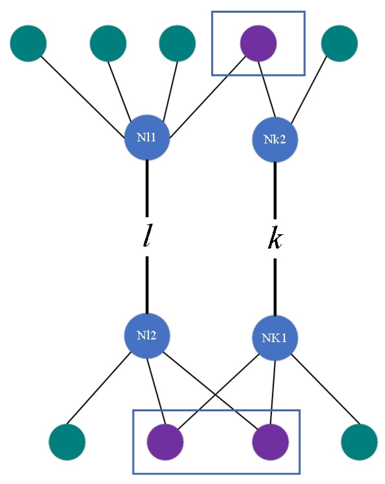
The edge-to-edge relation value is the mean distance of the attribute vector of the common adjacent nodes of the vertices of the two edges, as shown in Figure 2.
The vertices of edge l are Nl1 and Nl2, and the vertices of edge k are Nk1 and Nk2. The degrees of these four nodes are 4, 3, 3, and 2, respectively. Since the degree of Nl1 is greater than that of Nl2, and the degree of Nk2 is less than that of Nk1, we extract the common nodes of Nl1 and Nk2, and the common nodes of Nl2 and Nk1, to calculate the eigenvalue Dlk of these common node vectors, which represents the relationship value between edges l and k. The specific calculation process is as follows:
Extract the common adjacent nodes Clk of the two edges, as shown in Equation (2).
C l k = N max N l 1 , N l 2 min N k 1 , N k 2 N min N l 1 , N l 2 max N k 1 , N k 2
where N a b represents the common adjacency set of nodes a and b, max(i, j) represents the node with the larger number of adjacent nodes between i and j, and min(i, j) represents the node with the smaller number of adjacent nodes between i and j, as shown in Equations (3) and (4). M[i] indicates the number of nodes adjacent to node i.
max i , j = i ,       i f M i > M j j ,       o t h e r w i s e
min i , j = i ,       i f M i < M j j ,       o t h e r w i s e
Calculate the eigenvalue Dlk of the common adjacent node attribute vectors, as shown in Equation (5). This eigenvalue is the mean Euclidean distance of all common node attribute vectors, where P and Q are the attribute vectors of common adjacent nodes p and q, respectively.
D l k = p , q C l k P Q T P Q C l k C l k 1 2 ,       i f C l k C l k 1 2 > 0 0 ,       o t h e r w i s e

2.1.3. Constructing the Edge-Based Model

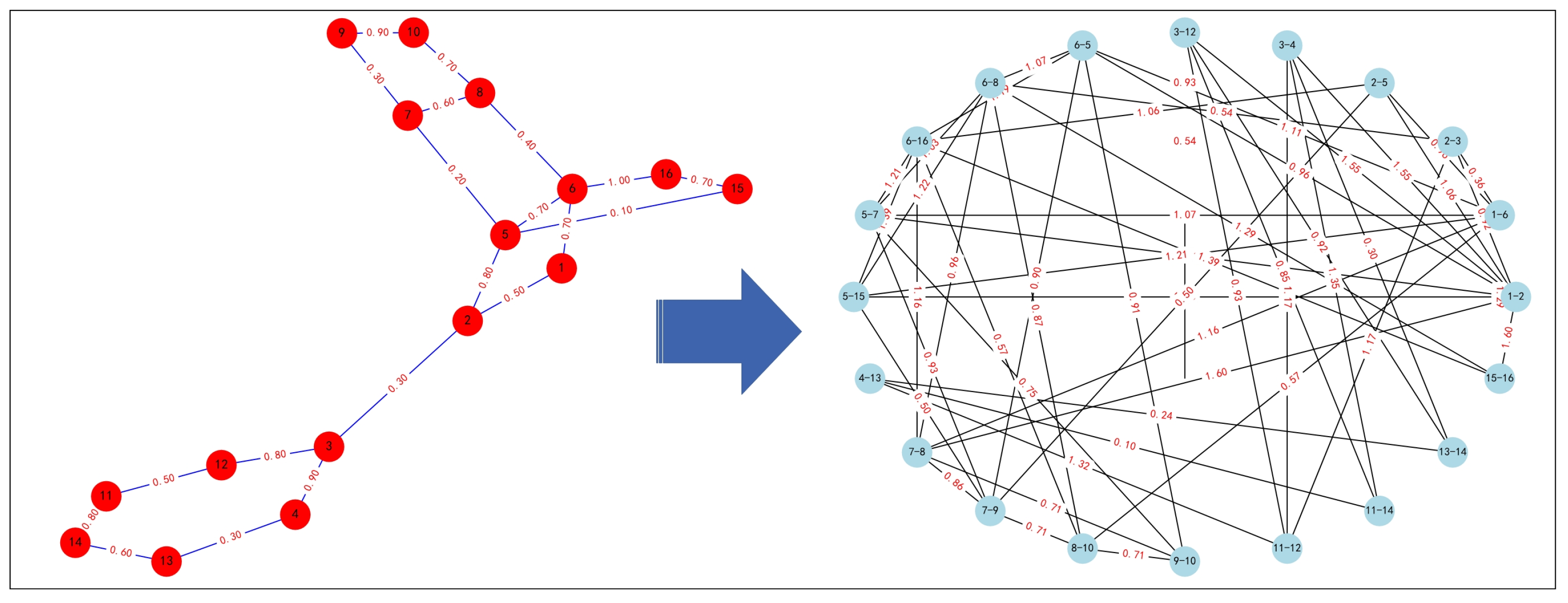
The edge eigenvalues calculated in Section 2.1.1 are used as the weights of the nodes in the edge-based model, and the relationship values between edges calculated in Section 2.1.2 are used as the weights of the edges in the edge-based model. The original network (node-based network) is transformed into an edge-based model, where nodes are the edges of the node-based network, and edges represent the relationships between edges in the node-based network. An example of a small network is shown in Figure 3. The network of blue nodes on the right is the edge-based model converted from the network of red nodes on the left. The edge-based model contains 16 nodes, which are the 16 edges in the node-based network. For example, node 3–12 in the edge-based model represents the edge between nodes 3 and 12 in the node-based network. The attribute vectors of the node-based network nodes are shown in Table 1.
The weights of the nodes in the edge-based model are shown in Table 2, where the numbers in the node numbers represent the vertex numbers of the edges in the node-based network. For example, node “1–2” represents the edge between vertices 1 and 2 in the node-based network.

2.2. Network Module Identification in Edge-Based Models

The module structure in complex networks refers to subsets or groups formed by tightly connected nodes [35,36]. Nodes within a module are closely connected, while connections between modules are sparse. Nodes within a module usually have similar functions or attributes [37,38]. Therefore, this paper assumes that nodes in the same module in the edge-based model should have the same dependent connection points. Identifying the module structure in the edge-based model mainly includes two steps: calculating node eigenvalues and clustering nodes.

2.2.1. Edge-Based Model Node Eigenvalues

Entropy is an important tool for measuring the disorder and information content of complex networks [39]. This paper uses the structural information entropy of edge-based model nodes as the eigenvalue of nodes. The eigenvalue ENi of node i is shown in Equation (6). λ is a weighting parameter. When its value is greater than 0.5, the node feature value emphasizes weight connectivity entropy. Conversely, when the value of λ is less than 0.5, the node feature value emphasizes weighted degree entropy. The value of λ needs to be manually set due to the significant differences among various types of complex system network models.
E N i = λ E H i + 1 λ E D i
EDi is the weighted degree entropy for each node i, as shown in Equation (7), where dj is the degree of a neighboring node j of node i.
E D i = j d j j d j log d j j d j
EHi is the weight connectivity entropy for node i, as shown in Equation (8), where ωij is the weight of edges connecting i to its neighbors j, and ε is a small value added to avoid log(0).
E H i = j ω i j j ω i j log ω i j j ω i j + ε

2.2.2. Edge-Based Model Clustering

Based on the eigenvalues of nodes in the edge-based model, the nodes are clustered. This paper uses the K-means algorithm for clustering. The K-means algorithm is a commonly used clustering algorithm that belongs to unsupervised learning [40]. The primary objective of the K-means algorithm is to partition the dataset into K clusters, ensuring that data points within the same cluster are as similar as possible, while those in different clusters are as distinct as possible. There are two main reasons for selecting this algorithm: first, it has a relatively low time complexity, making it suitable for handling large-scale datasets; second, the number of modules in the edge-based model can be determined by the number of dependent connections in the few-node network. The clustering process follows these steps:
  • Randomly select K nodes in the edge-based model as the initial cluster centers;
  • Assign each node to the nearest cluster center;
  • Recalculate the center of each cluster as the mean of all nodes assigned to it;
  • Repeat steps 2 and 3 until the cluster centers stabilize.

2.2.3. Module Eigenvalues in the Node-Based Network

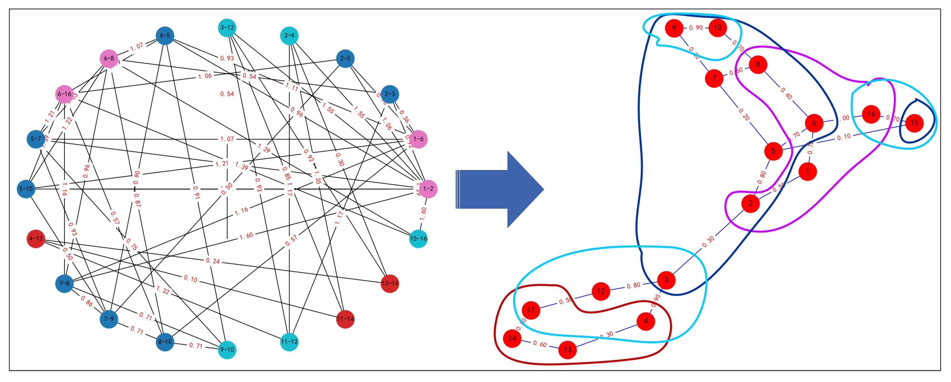
After clustering, each node in the edge-based model is assigned to a specific module. Since the nodes in the edge-based model correspond to edges in the node-based network, each node in the edge-based model is associated with two nodes in the node-based network. By assigning the nodes of the node-based network to the corresponding modules, based on the module affiliations of the edge-based model nodes, an overlapping modular structure of the node-based network is obtained. As illustrated in Figure 4, the left diagram displays the modular divisions of the edge-based model, with four modules, where nodes within the same module are color-coded. The right diagram in Figure 4 shows the modular divisions of the node-based network. The characteristic values of each module are provided in Table 3.
The characteristic value MDp of module p in the node-based network is the average number of adjacent nodes of all nodes in the module, as shown in Equation (9).
M D p = 1 N p i mod p j = 1 K n k i j
where modp is module p, Np is the number of nodes in module p, i is a node in module p, K is the adjacency matrix of the node-based network, and kij is the element value of K at row i and column j.

2.3. Characteristic Values of Few-Node Network Nodes

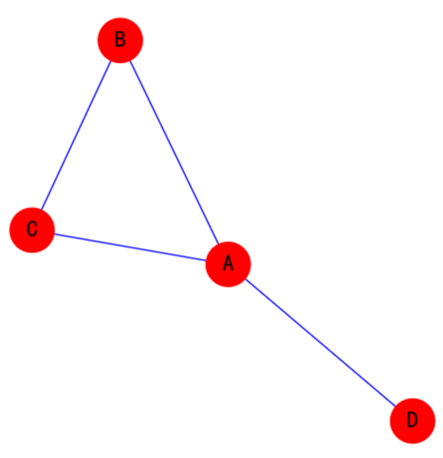
The characteristic value of a node in the few-node network is calculated based on the topological characteristics of the few-node network. This characteristic value is the weighted sum of the node degree and betweenness. Equation (10) expresses the characteristic value QTi of node i in the few-node network. As shown in Figure 5, the characteristic values of nodes A, B, C, and D in the network are 4.8, 1, 1, and 0.5, respectively.
Q T i = β j = 1 N A i j + δ s i t ν σ s t i σ s t
where Aij is the element of the adjacency matrix A, and N is the total number of nodes. Aij = 1 if there is an edge between nodes i and j; otherwise, Aij = 0. σst is the total number of shortest paths from node s to node t, and σst(i) is the number of those paths that pass through node i. β, δ, and ν are related calculation parameters, and their values can be adjusted according to the actual network characteristics. β and δ are weighting parameters. When the value of β is greater than δ, the calculation of the node feature value emphasizes the node’s weighted centrality. Conversely, when the value of β is less than δ, the calculation of the node feature value emphasizes the node’s information centrality. The parameter ν serves to adjust the magnitude of the results, ensuring that the calculation results of j = 1 N A i j and s i t ν σ s t i σ s t remain on the same scale.

2.4. Dependency Edge Prediction

The dependency degree between a module in the multi-node network and a node in the few-node network is calculated based on the characteristic values of the multi-node network modules and the few-node network nodes. The dependency degree represents the probability of a dependency relationship between a module in the multi-node network and a node in the few-node network. The higher the dependency degree, the higher the probability of a dependency relationship between them. If module M in the multi-node network has a dependency relationship with node A in the few-node network, it is considered that all nodes in module M have dependency edges with node A. The dependency degree ηMA between module M in the multi-node network and node A in the few-node network is shown in Equation (11).
η M A = 1 Q T M M D A
where Q T M and M D A are shown in Formula (12) and Formula (13), respectively.
Q T M = Q T M min Q T max Q T min Q T × 1 0.001 + 0.001
where Q T M is the eigenvalue of module M in the multi-node network, and min Q T and max Q T are, respectively, the minimum and maximum eigenvalue of all modules in the multi-node network.
M D A = M D A min M D max M D min M D × 1 0.001 + 0.001
where M D A is the eigenvalue of node A in the few-node network, and min M D and max M D are, respectively, the minimum and maximum eigenvalue of all modules in the few-node network.
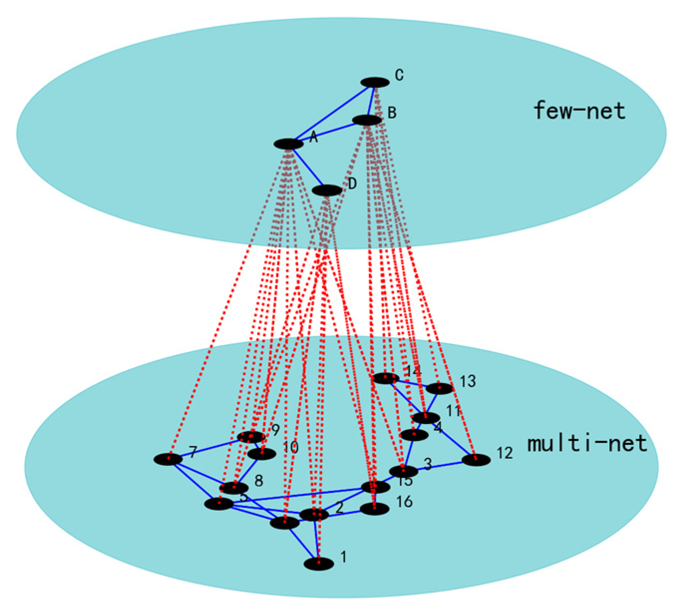
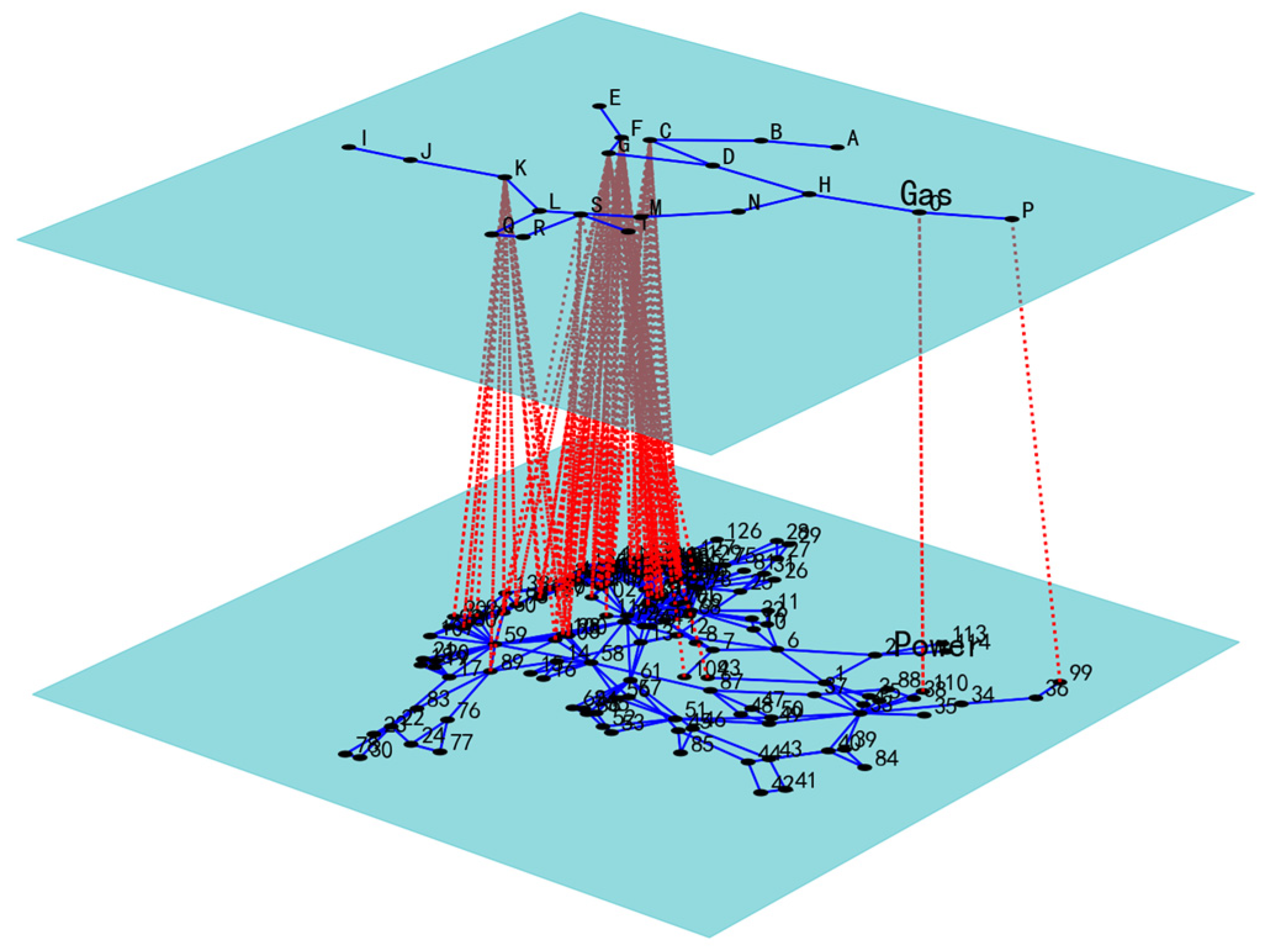
According to the above method, the dependency edge prediction results of the multi-node network in Section 2.1.3 and the few-node network introduced in Section 2.3 are shown in Figure 6. A total of 27 dependency edges were predicted. In Figure 6, the upper layer is the few-node network, the lower layer is the multi-node network, the black dots represent the nodes of the network, the blue solid lines are the edges in the network, and the red dashed lines are the dependency edges between the two networks.

3. Results and Discussion

In real life, most complex systems do not exist independently but are interconnected or interdependent. When nodes in interdependent complex systems suffer initial failures or attacks, the failures can propagate through the dependent systems, thereby gradually increasing the scale of the failures [41]. Structural prediction optimization can enhance the robustness of the systems [42]. To validate the effectiveness of the proposed dependency edge prediction method, we applied it to the prediction of dependency edges in power and gas networks, curriculum and competency networks, and content and question networks. These three types of dependency networks are abstracted from different domains. Although functionally distinct, they share structural characteristics as nonequilibrium dependency networks and exhibit many-to-many dependency patterns. Through this cross-domain validation, we aim to comprehensively evaluate the applicability and robustness of the proposed method across diverse dependency networks, thereby providing a solid foundation for future theoretical research and practical applications.

3.1. Power–Gas Network

With the increasing integration of gas-fired units in power systems, the interdependency between power and gas infrastructures has become highly intertwined. In 2019, the European Commission issued recommendations on network security in the energy sector, highlighting that the high degree of interconnection between gas and power systems amplifies the risk of interference and increases system vulnerability. Cascading failures, malicious attacks, and other disruptions can lead to catastrophic consequences. Therefore, constructing a robust joint operational dependency model for power and gas systems is essential to improving the reliability of these dependent infrastructure systems and effectively managing various emergencies and operational challenges. The peculiarity of the power system lies in its requirement for a real-time balance between generation and load, both under normal and fault conditions [43]. Any interruption in gas supply can significantly impact gas-fired power plants, potentially causing more severe blackouts than traditional emergencies in the power system.
The coupling between the power and gas systems occurs through generators, with the endpoints of the dependency edges being the generator nodes in the power grid and the load nodes in the gas network. A gas load node can supply gas to multiple generator nodes, and a generator node can receive gas from multiple gas load nodes, forming a many-to-many dependency pattern. Additionally, the number of nodes in the power network significantly exceeds that in the gas network, contributing to the nonequilibrium nature of the dependency system.

3.1.1. Power Network Model

The power network, a complex system, can be described and analyzed using a complex network model. In such a model, nodes represent various components of the power system, such as generators, transformers, and transmission lines, while edges represent the connections between these nodes, indicating energy transmission and information exchange within the system. The power network model can be divided into static and dynamic models. The static model primarily describes the structure and topological characteristics of the power grid, including node connectivity, network density, and node degree distribution. The dynamic model, on the other hand, describes the operational and control characteristics of the power grid, encompassing energy transmission, information exchange, and fault propagation among nodes. Through the complex network model, the stability, robustness, and reliability of the power network can be analyzed, offering theoretical support for grid planning, operation, and control. Furthermore, the model can be used to study fault-propagation mechanisms, vulnerability analysis, and recovery strategies, thereby providing insights into improving the disaster resilience and emergency response capabilities of the power grid.
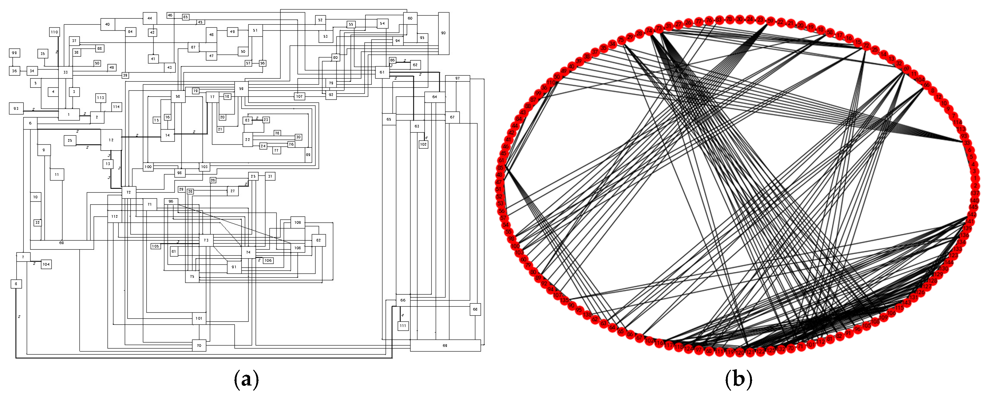
In this paper, a complex network model of the power network is constructed based on the IEEE_145 power grid line diagram, as shown in Figure 7. Figure 7a is the power network line diagram, and Figure 7b is the complex network model diagram. The network has 145 nodes and 422 edges. The nodes in the network are mainly divided into two types: one is the generator as the power source, and the other is the load node that receives power and transmits it to other substations or distributes it to other distribution substations in the local distribution network. The power network shown in Figure 7 has 50 generator nodes and 95 load nodes [44]. The network model can be represented by G, defined as graph G = (V, E), where V is the set of nodes (i.e., generators, transformers, substations, etc.), and E is the set of edges between nodes. The density of network G is 0.04, the average degree value is 5.82, and the average betweenness value is 0.0237. The model has the following characteristics:
  • All transmission lines are unique;
  • The attribute vector of nodes includes two values: voltage magnitude and voltage phase angle;
  • The weight of the transmission line is its reactance value.

3.1.2. Gas Network Model

The gas network is a complex system that transports gas from production sites to various consumption locations, ensuring safe and efficient transportation and usage of gas. This network typically consists of pipelines, compressor stations, pressure regulation stations, and storage facilities. Pipelines, usually made of steel or plastic, are used to transport high-pressure gas and are generally divided into trunk pipelines and branch pipelines. Trunk pipelines connect production sites and consumption locations, while branch pipelines connect trunk pipelines to specific consumers.
In the gas network, compressor stations play a crucial role. Compressor stations are used to increase the pressure of gas in the pipelines to ensure smooth flow. Additionally, pressure regulation stations are important facilities in the gas transmission network, used to adjust high-pressure gas to low-pressure gas suitable for consumer use. Furthermore, the gas network includes storage facilities to store gas to meet peak demand. These storage facilities typically include underground storage and liquefied gas storage facilities.
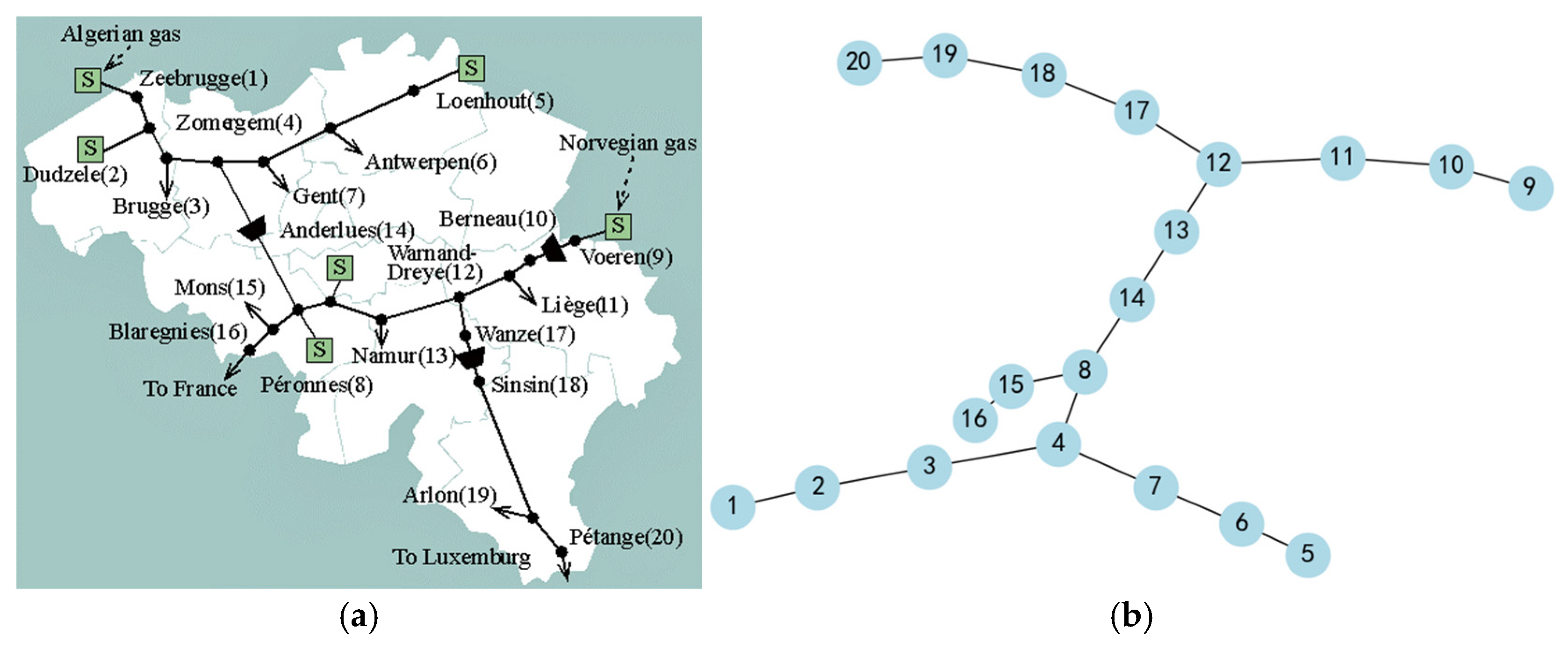
This paper adopts an improved Belgian 20-node gas network [45], which includes 6 gas source nodes, 8 load nodes, 23 gas pipelines, and three compressor stations. The system structure is shown in Figure 8a. We abstract gas source nodes, load nodes, and compressor station endpoints as nodes and transmission pipelines as edges to construct the gas network model, as shown in Figure 8b. The flow of pressure-driven gas through pipelines depends on factors such as pipeline length and diameter, operating temperature, gas composition, altitude changes along the transmission path, pipeline roughness, and boundary conditions. The transient flow of gas in pipelines is generally described as one-dimensional dynamics along the pipeline axis, requiring the use of distributed parameters and time-varying state variables, which will serve as the weight parameters of this network model.

3.1.3. Prediction Result of Power-Gas Network Dependent Edge

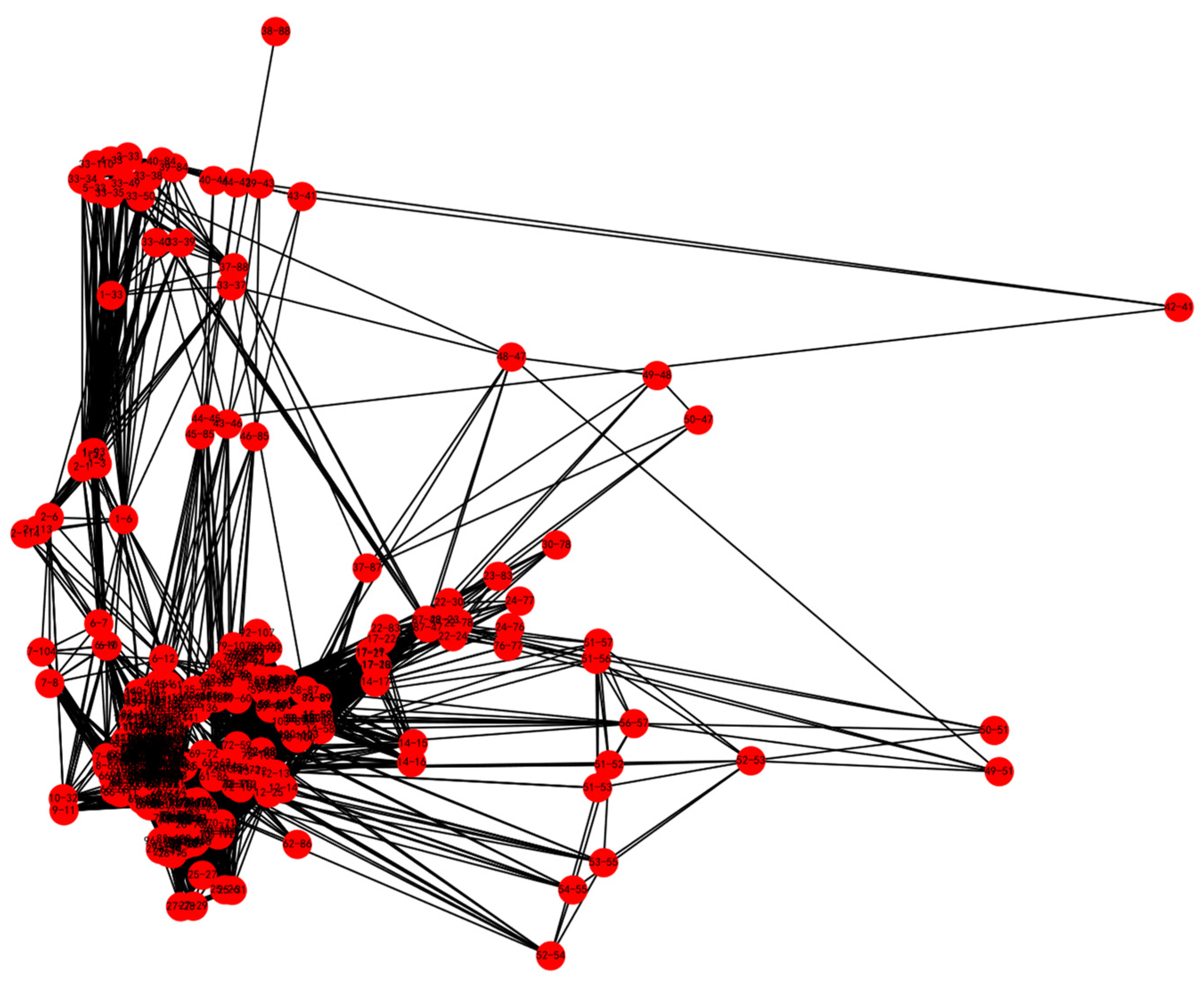
According to the method introduced in Section 2.1, we constructed the edge-based model of the power network, as shown in Figure 9. This network has 422 nodes and 24,782 edges, with 2 nodes having a degree of 0, which we removed, leaving 420 nodes. The edge-based model density is 0.282, the average degree is 118, the average betweenness is 0.0026, the average closeness is 0.497, and the average clustering coefficient is 0.721. Network density refers to the ratio of the number of actual edges to the maximum possible number of edges. The average degree is the mean value of the degrees of all nodes in the network. The degree of a node is the number of edges directly connected to that node. The average betweenness is the mean value of the betweenness of all nodes in the network. Node betweenness measures the proportion of shortest paths that pass through a node. The average closeness is the mean value of the closeness of all nodes in the network. Node closeness measures the average shortest path length from a node to all other nodes in the network. The average clustering coefficient is the mean value of the clustering coefficients of all nodes in the network. The clustering coefficient of a node measures the ratio of the number of actual edges between its neighbors to the maximum possible number of edges between them. The clustering coefficient reflects the tightness of connections among nodes in the network.
According to the method in Section 2.2.1, we calculated the weight connectivity entropy and weight degree entropy of each node in the edge-based model. Setting the weight to 0.3, we calculated the eigenvalues of the nodes in the edge-based model. Then, according to the method introduced in Section 2.2.2, we clustered the nodes in the edge-based model. Since there are eight load nodes in the gas network, the number of clusters is set to eight. According to the method introduced in Section 2.2.3, we divided the power network into eight modules based on the clustering results of the nodes in the edge-based model. The module attributes are shown in Table 4, where the module number is the name of the eight modules; the module nodes refer to the power grid nodes contained in the module, with red indicating generator node names; and the dependent edges of the power grid and gas network are the edges between generator nodes in the power grid and load nodes in the gas network. The average degree value refers to the average value of the unweighted degree values of all nodes in the power grid.
According to the method introduced in Section 2.3, we set the values of β and δ to 0.5 and the value of λ to 10, calculated the eigenvalues of each node in the gas network, extracted the matching nodes, and predicted the dependent relationships according to the method introduced in Section 2.4. The results are shown in Table 5, where the second row is the names of the matching nodes in the gas network, and the third row is the module numbers of the power network. The list in the table expresses the dependent relationships between nodes in the gas network and modules in the power network.
According to the principles introduced in Section 2.4, based on the dependent relationships in Table 5, we associated the nodes in the gas network with the nodes in the power network, predicting a total of 94 dependent edges, as shown in Table 6, where Tnet is the gas network node in the dependent edge, and Dnet is the power network node in the dependent edge. The power–gas dependent network constructed based on the prediction results of the dependent edges is shown in Figure 10.

3.1.4. Comparison of Robustness Evaluation Results

Infrastructure is a complex system susceptible to various threats such as natural disasters, equipment failures, and cyber-attacks. These disruptions can lead to widespread power outages, economic losses, and social chaos. Therefore, evaluating the robustness of infrastructure networks is crucial. Robustness analysis is a systematic method for assessing a system’s resilience to various disturbances and failures. It helps identify the impact of infrastructure network failures and develop strategies to enhance network resilience. By simulating different scenarios and analyzing the network’s response to interruptions, we can better understand the vulnerabilities of power networks and take measures to mitigate risks. This is essential for evaluating the resilience of infrastructure networks and ensuring the stability and security of power supply.
When interdependent infrastructures are damaged, one of the main concerns is determining the unmet load and quantifying the topological damage caused by such events. We focus on establishing a cascading failure propagation model for networks with mostly non-redundant equipment. When a node is attacked and fails, its load is transferred to its adjacent nodes. If the load of the adjacent nodes exceeds their capacity, they will also fail, resulting in a one-step cascading failure. If this impact continues to propagate, the entire network may experience a chain reaction, leading to network paralysis.
To verify the contribution of added interdependent edges to the robustness of the power–gas network, the attack targets should be the edges in the network. This paper adopts two attack strategies: random edge attacks and high-betweenness edge attacks. Based on three network robustness metrics—natural connectivity, geodesic vulnerability, and network efficiency—we compare the proposed interdependent edge prediction method with homogeneous and heterogeneous interdependent edge prediction methods to verify the effectiveness of our method. The interdependent edge prediction of homogeneous and heterogeneous networks is based on the closeness of nodes in the network, using a one-to-many interdependent edge connection mode.

Network Evaluation Metrics

Natural connectivity, geodesic vulnerability, and network efficiency are crucial metrics for evaluating the performance of complex networks. Natural connectivity measures the robustness and redundancy of a network by calculating the weighted sum of closed walks of different lengths within the network. Geodesic vulnerability assesses the network’s vulnerability by evaluating changes in the shortest path lengths following node or edge failures. Network efficiency, on the other hand, evaluates the transmission efficiency of a network by calculating the average of the reciprocals of the shortest path lengths between all pairs of nodes. Although all three metrics involve the calculation of path lengths and are used to assess network performance, they differ in their focus and computational methods. Natural connectivity is more suitable for networks requiring high reliability, geodesic vulnerability is better for assessing the network’s vulnerability to attacks or failures, and network efficiency is ideal for optimizing the speed of information transmission within the network.
1.
Natural Connectivity Metric
The natural connectivity metric of complex networks is used to measure the robustness or resilience of the network, i.e., the ability of the network to maintain its connectivity after nodes or edges are damaged. The natural connectivity metric has clear physical significance and a concise mathematical form, and it is easy to calculate. It can be directly derived from the spectral characteristics of the network’s adjacency matrix, reflecting the weighted sum of the number of closed loops of different lengths in the network, i.e., the redundancy of alternative paths in the network. The natural connectivity metric changes monotonically with the addition or deletion of edges and can be used to compare the robustness of different networks or different attack strategies [46,47].
A simple unweighted graph can be represented by an adjacency matrix A = (aij)N×N, where aij indicates the dependency strength between nodes i and j. If aij = 0, it means there is no edge between nodes i and j. Let ω1 ≥ ω2 ≥ … ≥ ωN be the eigenvalues of A, known as the spectral properties of the graph’s adjacency matrix. According to random matrix theory, the elements of the matrix An represent the number of paths connecting one node to another through n edges. The robustness of connections between nodes arises from the redundancy of alternative paths between them. Therefore, the robustness of a network can be considered to stem from the redundancy of alternative paths within the network. By representing the total number of closed paths in the network using the eigenvalues of the adjacency matrix, the robustness of the network can be expressed through the eigenvalues of the adjacency matrix, leading to the definition of the natural connectivity index as shown in the following Equation (14):
  ζ = ln 1 N i = 1 N e ω i
where ωi is the i-th eigenvalue of the network’s adjacency matrix, and N is the number of nodes in the network. The natural connectivity index calculates the closed paths between network nodes by considering the redundant paths between them. The higher the value of the index, the stronger the network’s robustness, indicating more alternative paths and higher network stability. The natural connectivity index, derived from the internal structural properties of complex networks, accurately captures subtle differences in network robustness by computing the weighted sum of closed paths of different lengths. It remains effective for disconnected graphs and can be directly derived from the spectral properties of the network’s adjacency matrix, possessing clear physical significance.
2.
Geodesic Vulnerability Index (GVI)
The GVI is a statistical measure used in the field of complex network theory, particularly suited for assessing the vulnerability of interdependent energy infrastructures. It aims to evaluate the structural vulnerability of these systems and identify infrastructure systems that are more prone to cascading failures. This method replaces traditional flow techniques by utilizing the geodesic vulnerability index to evaluate the robustness of infrastructure systems. In the evaluation process, a node is first disconnected, and then multiple cascading failures are simulated to assess the performance of the resulting topology. Through this approach, the topological performance of all nodes can be evaluated, and the damage area of each decomposition curve of cascading failures can be calculated to determine the system’s robustness [48].
This index is based on the concept of geodesic paths in graph theory, where a geodesic path is the shortest path between nodes in a network. In the context of energy infrastructure, these nodes can represent various components such as power plants or pipeline nodes. The higher the value of the geodesic vulnerability index, the greater the impact on the network due to congestion issues and cascading failures, as some geodesic paths are interrupted, forcing power to flow through other typically less efficient paths. This method has been used to assess the structural vulnerability of high-voltage power systems in countries such as Colombia and Spain, providing a new tool for infrastructure risk analysis and management. The GVI (κ) is as shown in Equation (15):
κ = 1 i j 1 / d i j L C i j 1 / d i j B C
where d i j L C is the geodesic distance between node pairs in the scale-free graph after removing a node; for the basic case, d i j B C is the geodesic distance between node pairs in the scale-free graph. The geodesic distance is defined as the shortest distance between two nodes, obtained by calculating the minimum number of nodes that must be traversed to connect the two nodes. The value of κ ranges between 0 and 1. The larger the value, the greater the impact on the dependent network.
3.
Network Efficiency Metric
Network efficiency is a necessary metric for measuring the information exchange between nodes in complex networks. It reflects the connectivity of the network; the better the connectivity, the less energy is consumed in interactions between nodes, and the more efficient the information transmission on the network. The efficiency between nodes is usually used to measure the speed of information transfer between nodes [49]. The definition of network efficiency η is given in Equation (16).
η = 1 N N 1 v i v j V 1 d i j
where dij represents the length of the shortest path between nodes vi and vj, and N denotes the total number of nodes in the network.

Random Edge Attacks

Random edge attacks involve randomly selecting an edge in the network for removal. This attack method does not require in-depth knowledge of the network’s specific information, making it relatively simple to implement. The results of the random edge attack process for the three interdependent networks are shown in Figure 11. Figure 11a, Figure 11b, and Figure 11c, respectively, show the changes in the natural connectivity metric, geodesic vulnerability metric, and network efficiency metric under random edge attacks for the three interdependent networks. The natural connectivity and network efficiency metrics are calculated using a cascading failure model, setting the initial weight of nodes in the interdependent network to one and the upper limit of nodes to twice the initial value.
As shown in the figure, before the attack, the values of the three robustness evaluation metrics—natural connectivity, geodesic vulnerability, and network efficiency—of the modular interdependent network are the highest. After seven random edge attacks, the values of the three robustness evaluation metrics of the modular interdependent network remain the highest, while the values of the three robustness evaluation metrics of the homogeneous and heterogeneous interdependent networks are close. At the same time, the slope of the change curve of the modular interdependent network under random edge attacks is relatively low. This indicates that under random edge attacks, the robustness of the power–gas interdependent network constructed using the interdependent edge prediction method proposed in this paper is superior to that of the power–gas interdependent networks constructed using the homogeneous and heterogeneous interdependent edge prediction methods.

High-Betweenness Edge Attacks

Edge betweenness is an important network analysis metric that measures the importance of an edge in the shortest paths between all pairs of nodes in the network. Specifically, edge betweenness refers to the proportion of the number of shortest paths passing through a particular edge to the total number of shortest paths in the network. The calculation formula for edge betweenness can be expressed as follows:
g v = s v t σ s t v σ s t
where σst is the number of shortest paths from node s to node t, and σst(v) is the number of these shortest paths passing through edge v.
High-betweenness edge removal attacks first require sorting the betweenness of edges after initializing the network. Then, in each round of attacks, we remove the edge with the highest betweenness. Finally, if multiple edges have the same betweenness, we randomly select one of them. The results of the high-betweenness edge attack process for the three interdependent networks are shown in Figure 12. Figure 12a, Figure 12b, and Figure 12c, respectively, show the changes in the natural connectivity metric, geodesic vulnerability metric, and network efficiency metric under high-betweenness edge attacks for the three interdependent networks. The natural connectivity and network efficiency metrics are calculated using a cascading failure model, setting the initial weight of nodes in the interdependent network to one and the upper limit of nodes to twice the initial value.
As shown in the figure, before the attack, the values of the three robustness evaluation metrics—natural connectivity, geodesic vulnerability, and network efficiency—of the modular interdependent network are the highest. After high-betweenness edge attacks, the values of the three robustness evaluation metrics of the modular interdependent network remain the highest, while the values of the three robustness evaluation metrics of the homogeneous and heterogeneous interdependent networks are close. At the same time, the slope of the change curve of the modular interdependent network under high-betweenness edge attacks is relatively low. This indicates that under high-betweenness edge attacks, the robustness of the power–gas interdependent network constructed using the interdependent edge prediction method proposed in this paper is superior to that of the power–gas interdependent networks constructed using the homogeneous and heterogeneous interdependent edge prediction methods.
In summary, the power–gas network constructed using the interdependent edge prediction method proposed in this paper exhibits superior robustness under both random and intentional attacks compared to that of the power–gas interdependent networks constructed using the homogeneous and heterogeneous interdependent edge prediction methods. This demonstrates that the proposed method can be effectively used for predicting interdependent edges in nonequilibrium complex systems such as power–gas infrastructure.

3.2. Course–Competency Network

Course learning is the key foundation for students to enhance their abilities. Courses that emphasize analytical reasoning, case studies, and project-based learning can help students develop critical thinking and problem-solving skills. Courses that require written assignments, presentations, and group collaborations help students improve their ability to clearly express their views and effectively collaborate with others. In fields such as engineering, computer science, and natural sciences, laboratory work, programming assignments, and practical workshops provide hands-on experience, enhancing students’ technical skills. Courses that include research methods, literature reviews, and independent research projects cultivate students’ research skills, encouraging them to explore, investigate, and contribute new knowledge to their fields. An educational system that integrates interdisciplinary learning into the curriculum encourages students to make connections across different fields, enhancing their interdisciplinary thinking abilities. Courses that include international perspectives, foreign languages, and global issues enable students to work effectively in multicultural environments and operate in the global market. Courses in philosophy, ethics, and social responsibility help students develop a strong sense of morality and ethical reasoning. Courses that include leadership training, team projects, and extracurricular activities help cultivate leadership and teamwork skills. Courses that include internships, cooperative projects, and industry partnerships provide students with practical experience, helping them apply theoretical knowledge to real-world situations.
The relationship between courses and the enhancement of students’ abilities is crucial for student development. The relationship between courses and competencies is not a simple one-to-one or one-to-many relationship; the study of one course can enhance multiple competencies in students, and the cultivation of one competency requires the support of multiple courses. Therefore, the relationship between courses and competencies is a typical many-to-many interdependent relationship. Moreover, from the training programs of various schools, it can be seen that the number of courses students need to complete far exceeds the number of competencies in the training objectives, so the course–competency interdependent network is a nonequilibrium network with a many-to-many interdependent model.

3.2.1. Course Network Model Construction

The course relationship network model is a model used to represent and analyze the relationships between courses. It can help teachers and students understand the structure and content of courses, as well as the dependencies and connections between courses. In the course relationship network model, nodes represent courses, edges represent the knowledge succession relationship between two courses, and the weight of the edges represents the degree of content succession between courses. Based on the training program of the electronics science major, we constructed a course network, including 52 nodes and 356 edges, as shown in Figure 13. The course names and their attribute vector values are shown in Table 7. The two values in the course attribute vector are the relevance values of the two cognitive process dimensions of knowledge understanding and application, and analysis and evaluation [50]. These two cognitive dimensions are based on the shared characteristics of the knowledge dimension and the cognitive process dimension as expressed in Bruner’s theory of cognitive structure learning [51]. The understanding dimension of understanding and application (DUA) refers to understanding meaning, transformation, rewriting, and explaining problems, where learners can express problems in their own words. Application refers to learners being able to apply the learned concepts to new situations or apply the learned knowledge to other scenarios [52]. The analysis dimension of analysis and evaluation (DAE) refers to breaking down material into its constituent parts to understand its organizational structure and determining how these parts are related to each other. Evaluation refers to students being able to make value judgments on a viewpoint based on certain evaluation criteria [52]. The density of this network is 0.268, the average degree value is 13.69, the average betweenness value is 0.015, the average closeness value is 0.577, and the average clustering coefficient is 0.509.
The code of the nodes in the figure is the sequence number of the course in Table 7.

3.2.2. Competency Network Model Construction

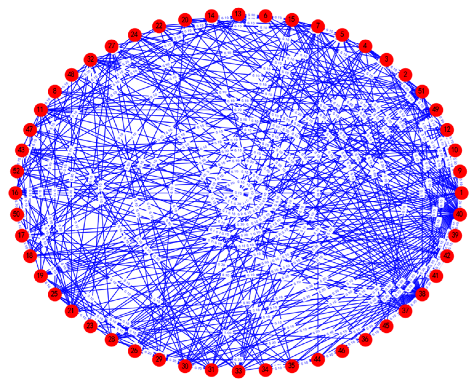
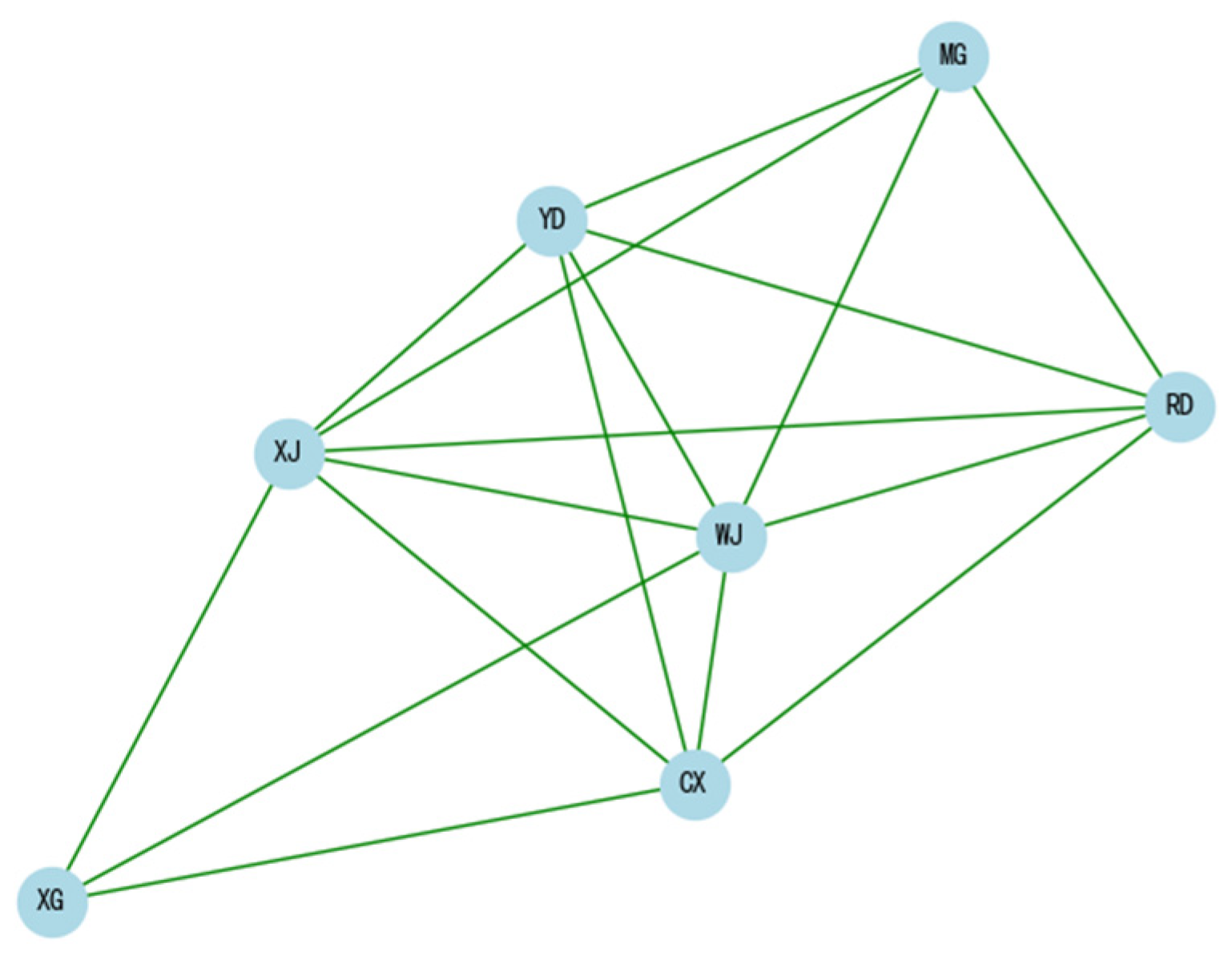
The general standards for engineering accreditation published by the China Engineering Education Accreditation Association are almost entirely consistent with the standards proposed by the Accreditation Board for Engineering and Technology (ABET) in the United States. This core competency framework provides the basic paradigm for the competency indicators in this paper. Based on the competency training objectives in the training program and the three-level competency indicators used for coding in the paper of [53], we extracted seven engineering practice competencies and constructed a competency relationship network model, as shown in Figure 14. This model is an undirected and unweighted network. The nodes in the network include the following:
  • Modeling competency: the ability to abstract and generalize the essence of engineering problems, establish mathematical and physical models of systems, and determine system performance indicators.
  • Hardware design competency: the ability to design hardware systems that meet requirements based on product needs and solve various problems encountered in the hardware design process.
  • Software development competency: the ability to write high-quality code, implement product functions, and debug and optimize software.
  • System integration competency: the ability to effectively integrate hardware and software to ensure the normal operation of the system.
  • Project management competency: the ability to effectively organize and manage the development process of projects, ensuring that projects are completed on time and with quality.
  • Innovation competency: the ability to continuously propose new ideas and solutions, promoting technological development and product innovation.
  • Problem-solving competency: the ability to quickly and accurately analyze and solve various technical and engineering problems.
    The edges in the network represent the relationships between various competencies.

3.2.3. Dependency Edge Prediction Results

According to the method introduced in Section 2.1, we constructed the edge-based model of the course network. The characteristic value Dlk of the common adjacent node attribute vector is the sum of the Euclidean distances of all common node attribute vectors, as shown in Formula (14), where P and Q are the attribute vectors of the common adjacent nodes p and q, respectively.
The constructed course edge-based model has 422 nodes and 62,873 edges. The mean value of all elements in this network is 27.37. To highlight the structural characteristics of the edge-based model, we optimized the edge-based model by deleting all edges with weights less than 27.37 and then deleting all nodes with a degree value of 0. The final course edge-based model has 349 nodes and 25,132 edges. The structural characteristics of the edge-based model before and after optimization are shown in Table 8, and the optimized edge-based model is shown in Figure 15.
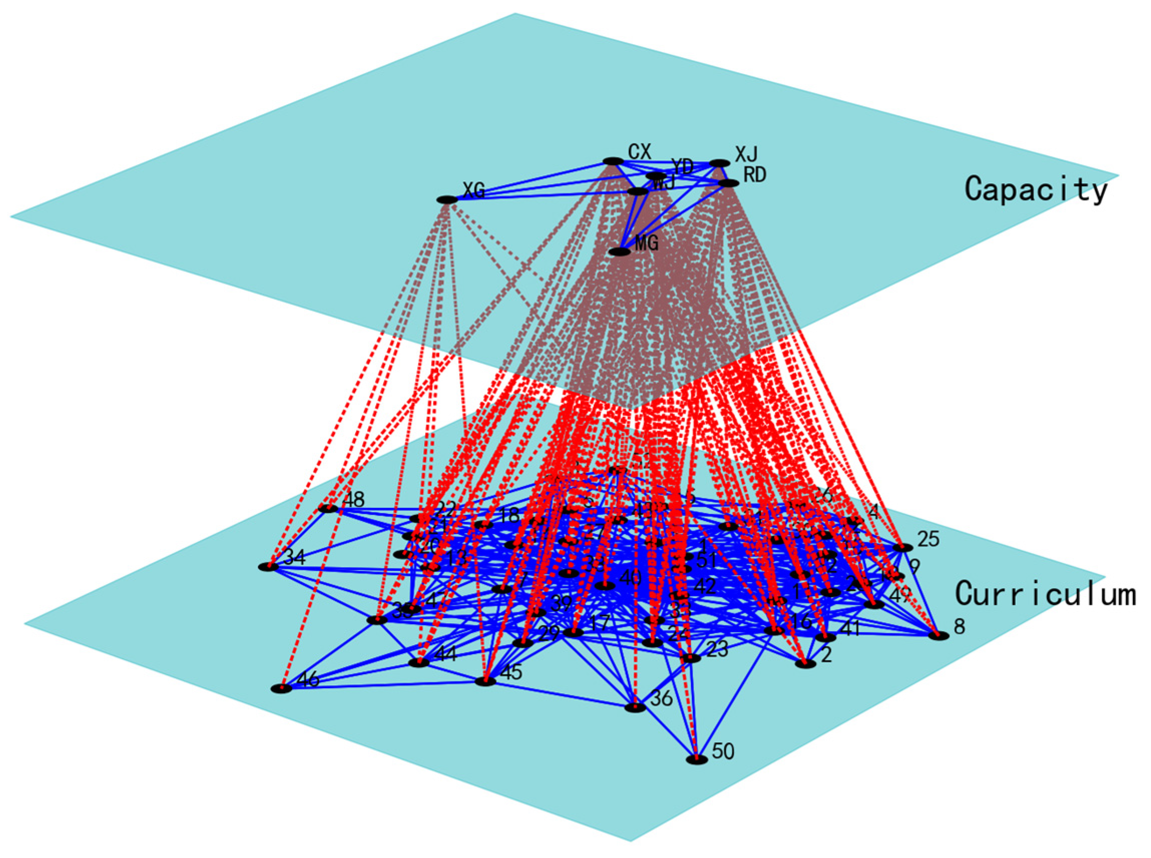
According to the method in Section 2.2.1, we calculated the weight connection entropy and weight degree entropy of each node in the edge-based model. Setting the weight to 0.5, we calculated the characteristic value of each node in the edge-based model. Then, according to the method introduced in Section 2.2.2, we clustered the nodes in the edge-based model. Since there are 349 nodes in the edge-based model, we set the number of clusters to 17 and divided the edge-based model into 17 modules. Next, according to the method introduced in Section 2.3, we set the values of β and δ to 0.5 and the value of λ to 100, calculated the characteristic value of each node in the competency network, and predicted the dependency relationships according to the method in Section 2.4. We identified the 7 modules most related to the seven nodes in the competency network from the 17 edge network modules and established dependency relationships. The results are shown in Table 9, where the first column is the competency node, the second column is the module with which it has a dependency relationship, the third column is the course nodes included in the module, and the fourth column is the average value of the unweighted degree values of all nodes in the course network.
According to the principles introduced in Section 2.4, based on the dependency relationships in Table 9, we associated the competency network nodes with the course network nodes and predicted a total of 170 dependency edges. The course–competency dependency network constructed according to the prediction results of the dependency edges is shown in Figure 16.

3.2.4. Comparison and Evaluation with Training Programs

We used the training programs of the electronics science and technology major from universities such as Beihua University as the standard to compare the course–competency support relationship results (i.e., dependency edges) predicted by this method with the course–competency corresponding relationships in the training programs to verify the validity of the prediction results.

Accuracy of Course and Competency Objectives

Course and competency objectives refer to the specific requirements in terms of knowledge, skills, and qualities that students need to achieve after completing a course. In this paper, the consistency indicator is used to measure the accuracy of the identified course and competency objectives. The accuracy of the competency objectives of course i, consistencyi, is shown in Formula (18).
c o n s i s t e n c y i = i n d e i r e a l e i r e a l e i × 100 %
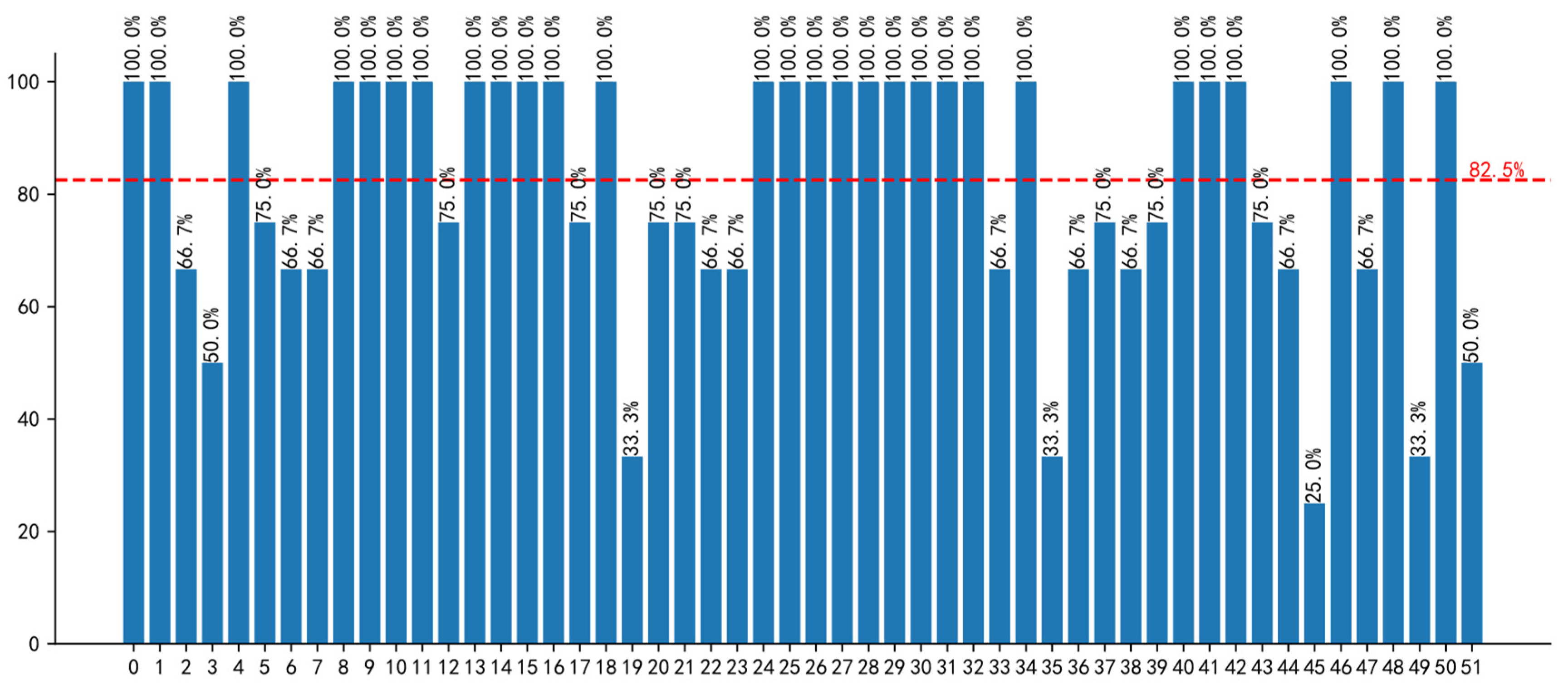
where indei is the predicted target competency set for course i, and realei is the actual competency target set for course i. The accuracy of the competency targets for the 52 courses is shown in Figure 17. The average accuracy for all courses is 82.5%, with 28 courses achieving 100% accuracy, indicating that the dependency edge prediction method proposed in this paper can accurately identify the competency targets of the courses.

Accuracy of Competency-Supporting Courses

Competency-supporting courses refer to those that directly support and achieve the talent cultivation competency targets within the curriculum system. These courses help students meet the graduation requirements and competency indicators set in the training program through specific teaching content and methods. The accuracy of identifying the supporting courses for competencyj, denoted as consistencyj, is measured using the consistency index as shown in Formula (19).
c o n s i s t e n c y j = c a d j r e a l c j r e a l c j × 100 %
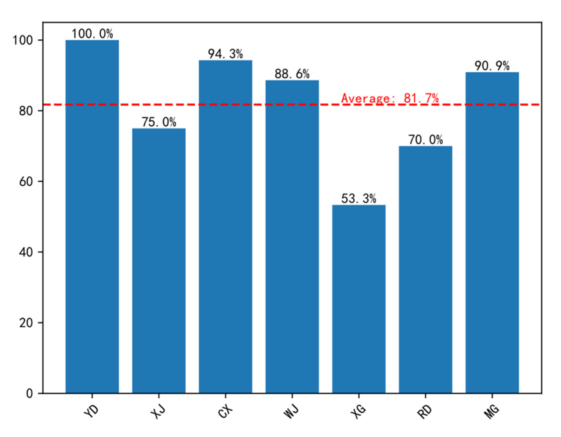
Among them, cadj is the predicted set of supporting courses for competency j, and realcj is the actual set of supporting courses for competency j. The accuracy of identifying the supporting courses for the seven competencies is shown in Figure 18, with an average accuracy of 81.7%. The accuracy for hardware development competency reaches 100%, and the accuracy for four competencies exceeds 85%, with only project management competency having a lower accuracy. This indicates that the dependency edge prediction method proposed in this paper can accurately identify the supporting relationships between courses and competency targets.
In summary, by using the dependency edge prediction method proposed in this paper to identify the supporting relationships between courses and competencies, the results show that the method can achieve effective prediction results for both the identification of course and competency targets and the identification of competency-supporting courses.

3.3. Text–Question Network

With the rapid development of artificial intelligence and the metaverse, intelligent answering has received widespread attention and application in the industry. Existing factual knowledge Q&A generally focuses on the progressive relationship between knowledge, without reflecting the cognitive relationship of the learning process. Moreover, semantic analysis of the question alone cannot evaluate the characteristics of the questioner, nor can it achieve quality enhancement of answers by gradually improving according to the personalized needs of the questioner. This requires strict answer screening methods, accurate questioner characteristic evaluation methods, and iterative question optimization methods to identify the personalized intentions of the questioner through multiple rounds of content enhancement, helping users obtain correct factual knowledge answers. Based on graph methods, the previous Q&A content is represented as a complex network model of words. By predicting the dependency relationship between the current question and the previous Q&A content network, key related keywords can be identified to optimize the current question and achieve personalized expression of the question.

3.3.1. Word Attribute Vectors

This paper uses the WebQuestions dataset [54,55] to validate the proposed method. The dataset was proposed by researchers at Stanford University in 2013 and contains 6642 pairs of questions and answers. The questions were obtained through the Google Suggest API, and the answers were obtained through Amazon Mechanical Turk, with all answers defined as Freebase entities. Before calculating the word attribute vectors, we preprocessed the text. First, we randomly selected 400 questions and performed sentence segmentation. A sentence is defined as any part of the text separated by a question mark. Next, we converted the text to lowercase; removed non-index words and punctuation; removed stop words such as “did”, “has”, “do”, “of”, “the”, “to”, etc.; replaced multiple spaces with a single space; and trimmed leading and trailing spaces.
After text preprocessing, we used the Word2Vec method [56] to calculate the word attribute vectors. Word2Vec is one of the earliest models to represent words as vectors, proposed by Google in 2013. Its goal is to train a neural network model to map each word to a vector representation in a high-dimensional vector space. Word2Vec mainly has two model architectures: Continuous Bag of Words (CBOW) and Skip-gram. The CBOW model predicts the center word from the context words. For example, given the context “the cat is on the”, the model predicts the word “mat” in the sentence “the cat is on the mat”. The Skip-gram model predicts the context words from the center word. For example, given the word “mat”, the model predicts the context “the cat is on the” in the same sentence. Word2Vec has two main training methods: Hierarchical Softmax and Negative Sampling. Hierarchical Softmax accelerates computation by constructing a Huffman tree, while Negative Sampling simplifies computation by sampling a small number of negative samples. This paper uses the Skip-gram model architecture and Hierarchical Softmax training method, setting the dimension of each vector to three and the maximum distance between the current word and the predicted word in a sentence to five.

3.3.2. Network Model Construction

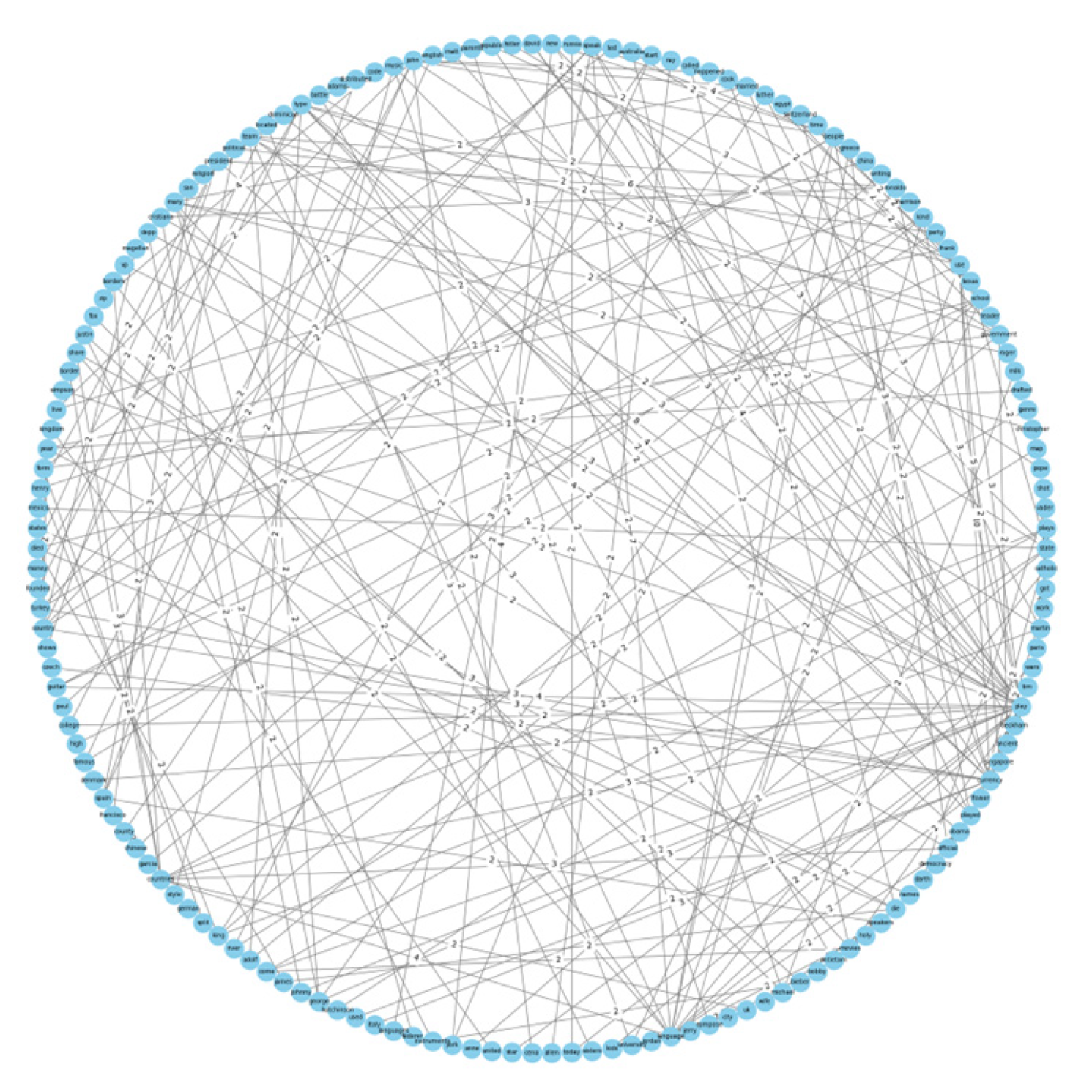
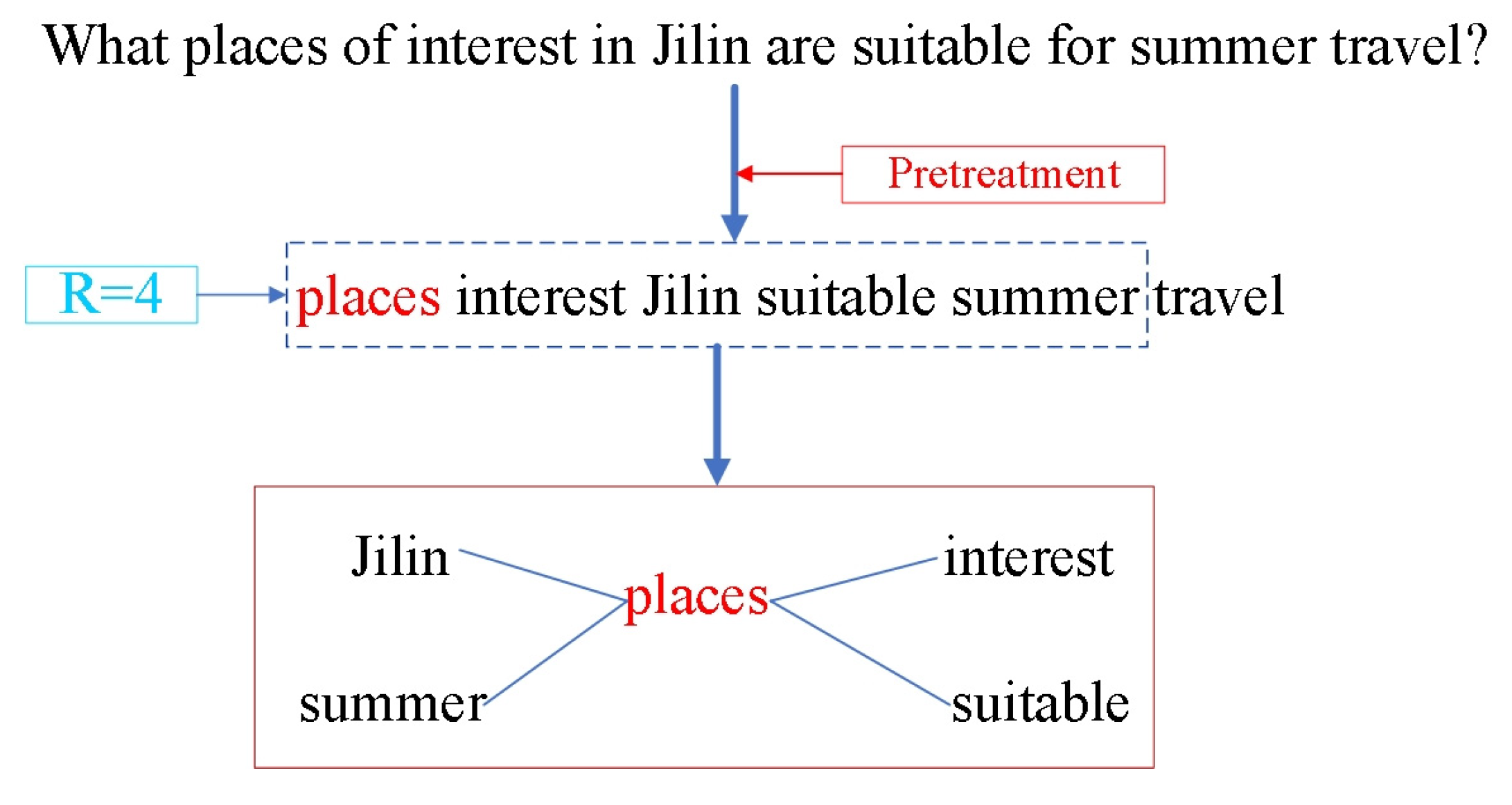
After calculating the word attribute vectors, we constructed a complex network model of the text. Each word in the text is treated as a node in the network model, and the domain relationship between two words is treated as an edge in the network model, i.e., a co-occurrence edge. The method for adding co-occurrence edges is to define an adjacency radius of size R and establish edges between all words coexisting within the adjacency radius. This paper sets the value of R to four, and the adjacency box slides along the text to add all edges. During the sliding process of the adjacency box, if the currently added edge is the same as an existing edge in the network, the weight of the edge is increased by one. After adding co-occurrence edges to the complex network model of the text, an undirected weighted complex network model is obtained [57]. Next, we processed the model by first deleting edges with weights less than two and then deleting nodes with a degree of 0. Finally, a complex network model with 158 nodes and 201 edges was obtained, as shown in Figure 19. Figure 20 shows an example of adding edges. After preprocessing the text, the adjacency nodes of “places” are extracted according to the size of the adjacency box radius, i.e., the four subsequent words of “places”, “interest”, “Jilin”, “suitable”, and “summer”. Therefore, we add four edges in the network model: “Jilin-places”, “summer-places”, “interest-places”, and “suitable-places”. Since there is already an edge with a weight of one in the network model, the weight of the edge is increased by one, making it two.

3.3.3. Dependent Edge Prediction Results

Following the method introduced in Section 2.1, we constructed the edge-based model of the text network. The feature values of the common adjacent node attribute vectors were the mean Euclidean distances of all common node attribute vectors. After obtaining the edge-based model, we deleted all nodes with a degree of 0. The final course edge-based model retained 188 nodes and 4870 edges, as shown in Figure 21. The edge-based model density was 0.277, the average degree was 51.809, the average betweenness was 0.0056, the average closeness was 0.47, and the average clustering coefficient was 0.527.
According to the method in Section 2.2.1, we calculated the weighted degree entropy and weighted connectivity entropy of each node in the edge-based model. Setting the weight to one, we calculated the feature values of the nodes in the edge-based model. Then, following the method introduced in Section 2.2.2, we clustered the nodes in the edge-based model. Since there were 188 nodes in the edge-based model, we set the number of clusters to 20. According to the method introduced in Section 2.2.3, based on the clustering results of the nodes in the edge-based model, we divided the text network into 20 modules. The module attributes are shown in Table 10, where the module number is the name of the 20 modules, the module nodes are the names of the word nodes contained in the module, and the average degree is the average unweighted degree of all nodes in the text network.
Taking the randomly input question “The roles played by movie actors and their countries” as an example, we constructed the network model of the question according to the method in Section 3.3.1. Then, following the method introduced in Section 2.3, we calculated the feature values of each node in the question network, with both β and δ set to 0.5, and λ set to 10. Next, according to the method introduced in Section 2.4, we performed dependency relationship prediction, and the results are shown in Table 11. The second row of the table has the words in the question sentence, i.e., the nodes of the question network; the third row is the module number of the text network. The list in the table expresses the dependency relationship between the nodes of the question network and the modules of the text network.
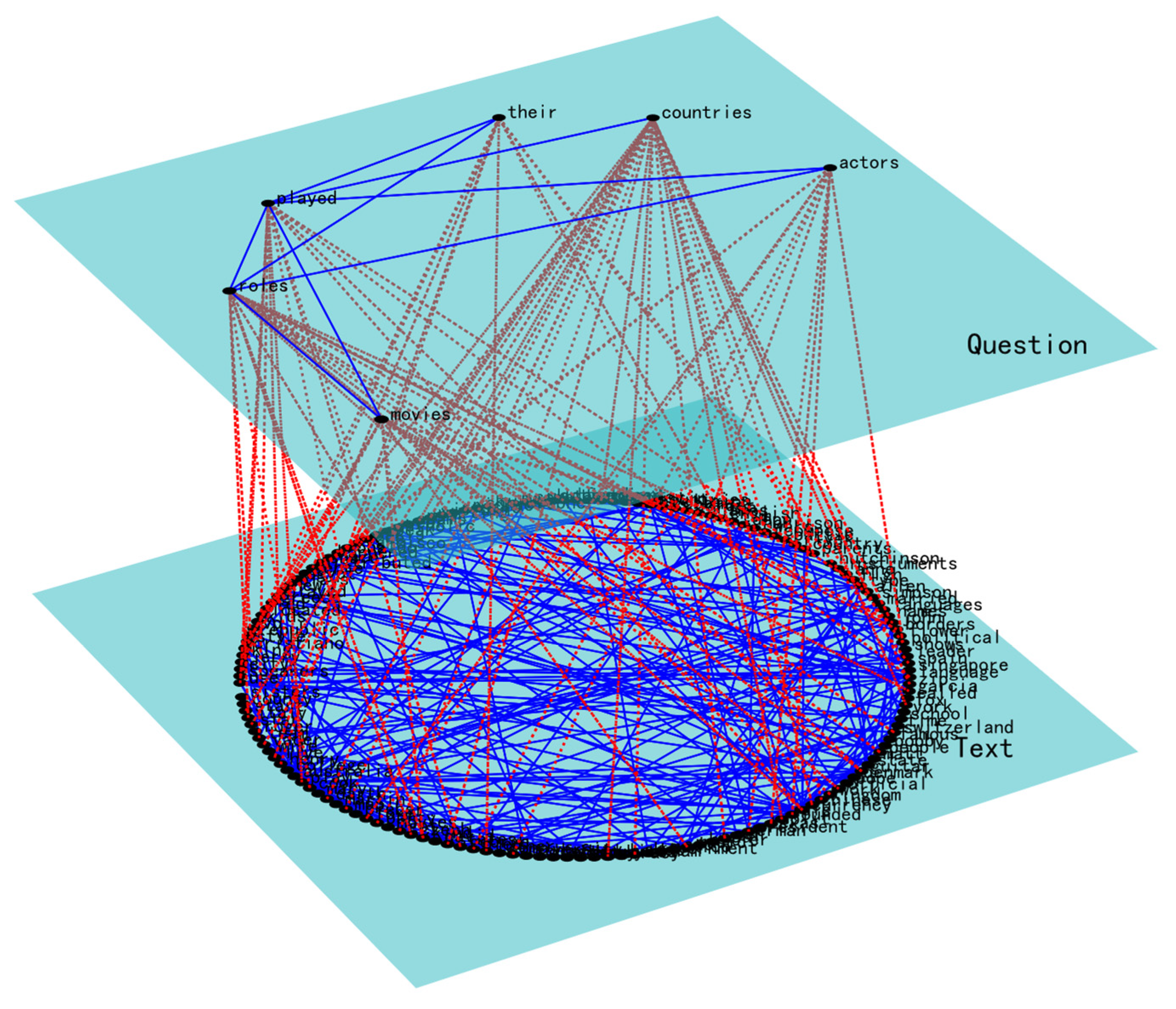
According to the principles introduced in Section 2.4, based on the dependency relationships in Table 11, we associated the capability network nodes with the course network nodes, predicting a total of 92 dependent edges. The text–question dependency network constructed based on the predicted dependent edges is shown in Figure 22.

3.3.4. Experimental Comparison Results

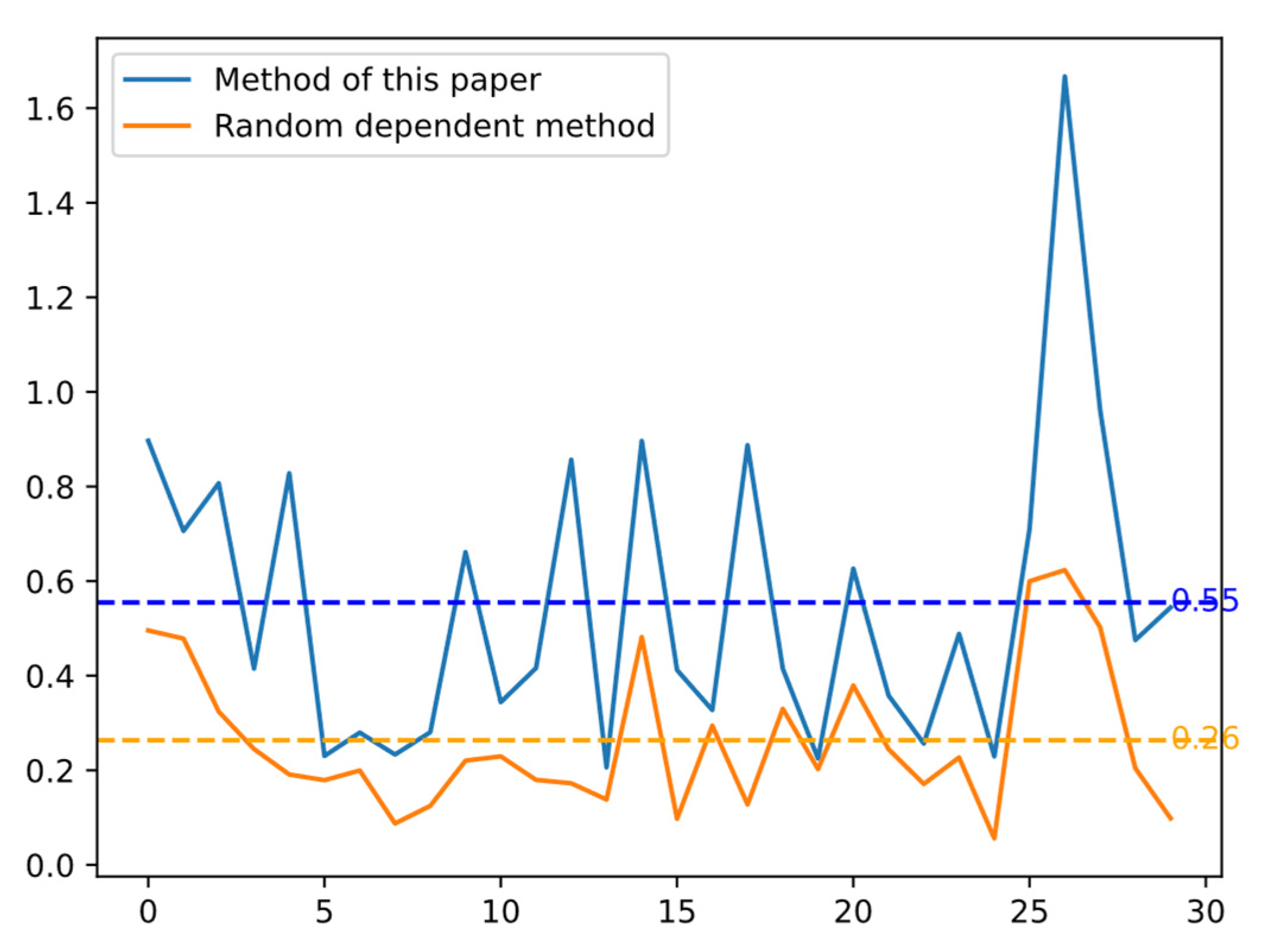
To verify the effectiveness of the dependency edge prediction method proposed in this paper in the field of text recognition, we constructed 30 question network models with 30 different question sentences, predicting the dependency relationships between the core nodes in the question networks and the text network nodes constructed in Section 3.3.1, obtaining dependent vocabularies. In the prediction method, the number of modules in the text edge-based model was not less than the number of nodes in the question network. Then, using the information gain method [58,59], we calculated the average information gain of the dependent vocabularies and the question sentences to measure the accuracy of the dependency relationship prediction. The information gain method measures the importance of a feature word by the increase in information in the corpus before and after the presence of the feature word. We compared our method with the random dependency method. The feature values of the question network nodes were calculated according to the method introduced in Section 2.3, with β set to 0.2, δ set to 0.8, and λ set to 10. The random dependency method randomly establishes one-to-one dependency relationships between the nodes in the question network and the nodes in the text network. The information gain results of the 30 questions are shown in Figure 23. The blue curve in the figure represents the information gain values of the text and question sentences obtained using the dependency edge prediction method proposed in this paper, while the orange curve represents the information gain values obtained using the random dependency edge prediction method. The blue dashed line is the mean line of the blue curve, with a mean value of 0.55, and the orange dashed line is the mean line of the orange curve, with a mean value of 0.25. The information gain values obtained by the prediction method proposed in this paper are all higher than those obtained by the random dependency prediction method, indicating that the prediction method proposed in this paper can be applied to the field of intelligent question answering to identify keywords related to the question sentences.

4. Conclusions

The models of complex dependent systems are usually very complex, involving multiple subsystems and various dependency relationships. This paper proposes a dependency edge prediction method based on overlapping module features for the network model of nonequilibrium dependent complex systems. This method aims to solve the problem of many-to-many dependency relationship prediction between multi-domain nonequilibrium complex networks. First, the point network model of the heavy network is converted into an edge-based model. Then, based on the topological structure of the edge-based model, clustering is performed to identify the module structure of the edge-based model. Since a node in the edge-based model corresponds to two nodes in the point network, mapping the module structure of the edge-based model to the point network model results in an overlapping module structure. Next, based on the topological structure features, the structural feature values of each module in the point network model and the node feature values of the light network are calculated. The proximity of the node feature values is used as the probability of the existence of dependent edges, achieving many-to-many dependency edge prediction.
We applied it to the dependency edge prediction of power and gas networks, course and capability networks, and text and question networks. The power and gas network is a model of the power–gas system, where the power generation nodes in the network use natural gas for power generation. To achieve the transmission of natural gas, it is necessary to associate the load nodes of the gas network with the power generation nodes of the power network. These dependency relationship connection patterns can affect the robustness of the system. Course learning is the main way for students to improve their abilities. A course often supports multiple capability goals, and a capability goal often requires the support of multiple courses. The number of courses is generally much larger than the number of capability goals. Therefore, identifying the support relationships between courses and capabilities is a typical many-to-many dependency relationship prediction problem in nonequilibrium dependent networks. Text is the basis of intelligent question answering, and questions are the main medium of communication between humans and machines. By taking individual words as nodes and the relationships between words as edges, text and question network models can be constructed. Predicting the dependency relationships between question nodes and text nodes can provide an effective basis for optimizing questions. These three dependency networks are abstracted from different fields. Although they are completely different in function, they are all nonequilibrium dependent networks in structure and exhibit many-to-many dependency patterns. Through this cross-domain verification, we can comprehensively evaluate the applicability and robustness of the proposed method in different types of dependent networks, providing a solid foundation for further theoretical research and practical applications.
The application results in these three types of interdependent networks demonstrate that the proposed dependency edge prediction method effectively enhances the robustness of the interdependent network in the power–gas network, accurately identifies the supporting relationships between courses and competencies in the course–competency network, and achieves good information gain values in the text–question network. These results validate that the proposed method, based on overlapping modular characteristics, can effectively predict dependency relationships in various unbalanced complex systems across different fields. However, the proposed method has certain limitations. First, the method is applied to undirected networks, requiring the transformation of complex systems into undirected complex network models, which necessitates ignoring the directionality of relationships between elements in complex systems. Second, the method requires converting node networks into edge networks before module identification, which demands high time and space resources for high-density, large-scale complex systems. Therefore, optimizing the conversion method from node networks to edge networks is necessary to improve computational efficiency for high-density, large-scale complex systems. Third, while the method can be applied to complex systems in different fields, the significant differences in the attributes of elements and relationships in complex systems across different fields necessitate adjusting parameters such as ω, β, and δ according to the specific network model when applying this method.

Author Contributions

Conceptualization, Q.Z.; methodology, Q.Z. and L.Y.; software, Q.Z.; validation, Q.Z., L.Y. and Y.G.; formal analysis, Q.Z.; investigation, J.H.; resources, Q.Z.; data curation, Q.Z.; writing—original draft preparation, Q.Z.; writing—review and editing, Q.Z.; visualization, Q.Z.; supervision, Q.Z.; project administration, Q.Z; funding acquisition, Q.Z. All authors have read and agreed to the published version of the manuscript.

Funding

This research was funded by Jilin Provincial Natural Science Foundation: Research on Iterative Answer Personalization Enhancement Method Based on Heterogeneous Relationship Networks, grant number 20230101238JC; Jilin Provincial Higher Education Teaching Reform Research Project: Research on the Value-Added Model of Practical Ability of Applied Information Students in the Post-Pandemic Era, grant number JLJY202377910357; and Beihua University 2024 School-Level Education and Teaching Reform Research Project: Research on the Construction of Intelligent Information Processing Courses Catalyzed by Interdisciplinary Integration, grant number 21xjyb-1241695.

Data Availability Statement

The data and computer programs involved in this paper can be requested at [email protected].

Conflicts of Interest

The funders had no role in the design of this study; in the collection, analyses, or interpretation of data; in the writing of the manuscript; or in the decision to publish the results.

References

  1. Amini, M.H.; Boroojeni, K.G.; Iyengar, S.S.; Blaabjerg, F.; Pardalos, P.M.; Madni, A.M. (Eds.) A Panorama of Future Interdependent Networks: From Intelligent Infrastructures to Smart Cities. In Sustainable Interdependent Networks: From Theory to Application; Springer: Cham, Switzerland, 2018; Volume 145, pp. 1–10. [Google Scholar]
  2. Sarwat, A.I.; Sundararajan, A.; Parvez, I.; Moghaddami, M.; Moghadasi, A. Toward a Smart City of Interdependent Critical Infrastructure Networks. In Sustainable Interdependent Networks: From Theory to Application; Amini, M.H., Boroojeni, K.G., Iyengar, S.S., Pardalos, P.M., Blaabjerg, F., Madni, A.M., Eds.; Springer International Publishing Ag: Cham, Switzerland, 2018; Volume 145, pp. 21–45. [Google Scholar]
  3. Buldyrev, S.V.; Parshani, R.; Paul, G.; Stanley, H.E.; Havlin, S. Catastrophic cascade of failures in interdependent networks. Nature 2010, 464, 1025–1028. [Google Scholar] [CrossRef] [PubMed]
  4. Zhang, C.; Lei, Y.; Shen, X.; Li, Q.; Yao, H.; Cheng, D.; Xie, Y.; Yu, W. Fragility Induced by Interdependency of Complex Networks and Their Higher-Order Networks. Entropy 2022, 25, 22. [Google Scholar] [CrossRef] [PubMed]
  5. Chen, C.-Y.; Zhao, Y.; Gao, J.; Stanley, H.E. Nonlinear model of cascade failure in weighted complex networks considering overloaded edges. Sci. Rep. 2020, 10, 13428. [Google Scholar] [CrossRef] [PubMed]
  6. Zhang, Z.; Yin, Y.; Zhang, X.; Liu, L. Optimization of robustness of interdependent network controllability by redundant design. PLoS ONE 2018, 13, e0192874. [Google Scholar] [CrossRef] [PubMed]
  7. Chen, D.B.; Lü, L.Y.; Shang, M.S.; Zhang, Y.C.; Zhou, T. Identifying influential nodes in complex networks. Phys. A-Stat. Mech. Its Appl. 2012, 391, 1777–1787. [Google Scholar] [CrossRef]
  8. Wang, X.; Cao, J.; Li, R.; Zhao, T. A preferential attachment strategy for connectivity link addition strategy in improving the robustness of interdependent networks. Phys. A-Stat. Mech. Its Appl. 2017, 483, 412–422. [Google Scholar] [CrossRef]
  9. Beygelzimer, A.; Grinstein, G.E.; Linsker, R.; Rish, I. Improving network robustness by edge modification. Phys. A-Stat. Mech. Its Appl. 2005, 357, 593–612. [Google Scholar] [CrossRef]
  10. Jiang, Z.Y.; Liang, M.G.; Guo, D.C. Enhancing network performance by edge addition. Int. J. Mod. Phys. C 2011, 22, 1211–1226. [Google Scholar] [CrossRef]
  11. Sydney, A.; Scoglio, C.; Gruenbacher, D. Optimizing algebraic connectivity by edge rewiring. Appl. Math. Comput. 2013, 219, 5465–5479. [Google Scholar] [CrossRef]
  12. Cao, X.B.; Hong, C.; Du, W.B.; Zhang, J. Improving the network robustness against cascading failures by adding links. Chaos Solitons Fractals 2013, 57, 35–40. [Google Scholar] [CrossRef]
  13. Ji, X.; Wang, B.; Liu, D.; Chen, G.; Tang, F.; Wei, D.; Tu, L. Improving interdependent networks robustness by adding connectivity links. Phys. A-Stat. Mech. Its Appl. 2016, 444, 9–19. [Google Scholar] [CrossRef]
  14. Chen, C.Y.; Zhao, Y.; Qin, H.; Meng, X.; Gao, J. Robustness of interdependent scale-free networks based on link addition strategies. Phys. A-Stat. Mech. Its Appl. 2022, 604, 127851. [Google Scholar] [CrossRef]
  15. Lao, S.; Wang, J.; Bai, L. Review of the interdependent networks. J. Natl. Univ. Def. Technol. 2016, 38, 122–128. [Google Scholar]
  16. Gao, J.X.; Barzel, B.; Barabasi, A.L. Universal resilience patterns in complex networks. Nature 2016, 530, 307–312. [Google Scholar] [CrossRef]
  17. Valdez, L.D.; Shekhtman, L.; La Rocca, C.E.; Zhang, X.; Buldyrev, S.V.; Trunfio, P.A.; Braunstein, L.A.; Havlin, S.; Estrada, E. Cascading failures in complex networks. J. Complex Netw. 2020, 8, cnaa013. [Google Scholar] [CrossRef]
  18. Son, S.-W.; Bizhani, G.; Christensen, C.; Grassberger, P.; Paczuski, M. Percolation theory on interdependent networks based on epidemic spreading. Epl 2012, 97, 16006. [Google Scholar] [CrossRef]
  19. Min, B.; Do Yi, S.; Lee, K.-M.; Goh, K.I. Network robustness of multiplex networks with interlayer degree correlations. Phys. Rev. E 2014, 89, 042811. [Google Scholar] [CrossRef] [PubMed]
  20. Watanabe, S.; Kabashima, Y. Cavity-based robustness analysis of interdependent networks: Influences of intranetwork and internetwork degree-degree correlations. Phys. Rev. E 2014, 89, 012808. [Google Scholar] [CrossRef]
  21. Min, B.; Lee, S.; Lee, K.-M.; Goh, K.I. Link overlap, viability, and mutual percolation in multiplex networks. Chaos Solitons Fractals 2015, 72, 49–58. [Google Scholar] [CrossRef]
  22. Cellai, D.; Dorogovtsev, S.N.; Bianconi, G. Message passing theory for percolation models on multiplex networks with link overlap. Phys. Rev. E 2016, 94, 032301. [Google Scholar] [CrossRef]
  23. Shao, S.; Huang, X.; Stanley, H.E.; Havlin, S. Robustness of a partially interdependent network formed of clustered networks. Phys. Rev. E 2014, 89, 032812. [Google Scholar] [CrossRef] [PubMed]
  24. Liu, X.; Pan, L.; Stanley, H.E.; Gao, J. Multiple phase transitions in networks of directed networks. Phys. Rev. E 2019, 99, 012312. [Google Scholar] [CrossRef] [PubMed]
  25. Li, W.; Bashan, A.; Buldyrev, S.V.; Stanley, H.E.; Havlin, S. Cascading Failures in Interdependent Lattice Networks: The Critical Role of the Length of Dependency Links. Phys. Rev. Lett. 2012, 108, 228702. [Google Scholar] [CrossRef]
  26. Kleineberg, K.-K.; Buzna, L.; Papadopoulos, F.; Boguna, M.; Serrano, M.A. Geometric Correlations Mitigate the Extreme Vulnerability of Multiplex Networks against Targeted Attacks. Phys. Rev. Lett. 2017, 118, 218301. [Google Scholar] [CrossRef]
  27. Danziger, M.M.; Bonamassa, I.; Boccaletti, S.; Havlin, S. Dynamic interdependence and competition in multilayer networks. Nat. Phys. 2019, 15, 178–185. [Google Scholar] [CrossRef]
  28. Xu, X.; Fu, X. Analysis on Cascading Failures of Directed-Undirected Interdependent Networks with Different Coupling Patterns. Entropy 2023, 25, 471. [Google Scholar] [CrossRef]
  29. Zhou, L.; Yin, J.; Tan, F.; Liao, H. Robustness analysis of edge-coupled interdependent networks under different attack strategies. Phys. A-Stat. Mech. Its Appl. 2023, 632, 129338. [Google Scholar] [CrossRef]
  30. Peng, H.; Zhao, Y.; Zhao, D.; Zhong, M.; Hu, Z.; Han, J.; Li, R.; Wang, W. Robustness of higher-order interdependent networks. Chaos Solitons Fractals 2023, 171, 113485. [Google Scholar] [CrossRef]
  31. Modarresi, A.; Symons, J. Modeling Technological Interdependency in IoT—A Multidimensional and Multilayer Network Model for Smart Environments; IEEE: New York, NY, USA, 2019; pp. 1–7. [Google Scholar]
  32. Tu, H.; Xia, Y.; Wu, J.; Zhou, X. Robustness assessment of cyber-physical systems with weak interdependency. Phys. A-Stat. Mech. Its Appl. 2019, 522, 9–17. [Google Scholar] [CrossRef]
  33. Zhou, S.H.; Ng, S.T.; Yang, Y.F.; Xu, F.J.; Li, D.Z. A Data-Driven and Physics-Based Approach to Exploring Interdependency of Interconnected Infrastructure; The American Society of Civil Engineers: New York, NY, USA, 2019; pp. 82–88. [Google Scholar]
  34. Cao, Y.-Y.; Liu, R.-R.; Jia, C.-X.; Wang, B.-H. Percolation in multilayer complex networks with connectivity and interdependency topological structures. Commun. Nonlinear Sci. Numer. Simul. 2021, 92, 105492. [Google Scholar] [CrossRef]
  35. Guimera, R.; Sales-Pardo, M.; Amaral, L.A.N. Module identification in bipartite and directed networks. Phys. Rev. E 2007, 76, 036102. [Google Scholar] [CrossRef] [PubMed]
  36. Gonzalez, M.C.; Barabasi, A.-L. Complex networks—From data to models. Nat. Phys. 2007, 3, 224–225. [Google Scholar] [CrossRef] [PubMed]
  37. Shi, D.; Shang, F.; Chen, B.; Expert, P.; Lue, L.; Stanley, H.E.; Lambiotte, R.; Evans, T.S.; Li, R. Local dominance unveils clusters in networks. Commun. Phys. 2024, 7, 170. [Google Scholar] [CrossRef]
  38. Xie, J.; Meng, F.; Sun, J.; Ma, X.; Yan, G.; Hu, Y. Detecting and modelling real percolation and phase transitions of information on social media. Nat. Hum. Behav. 2021, 5, 1161–1168. [Google Scholar] [CrossRef]
  39. Stella, M.; De Domenico, M. Distance Entropy Cartography Characterises Centrality in Complex Networks. Entropy 2018, 20, 268. [Google Scholar] [CrossRef] [PubMed]
  40. Gao, Z.; Jin, N.; IEEE. Detecting community structure in complex networks based on K-means clustering and data field theory. In Proceedings of the 2008 Chinese Control and Decision Conference, Yantai, China, 2–4 July 2008; pp. 4411–4416. [Google Scholar]
  41. Jiang, W.-J.; Liu, R.-R.; Fan, T.-L.; Liu, S.-S.; Lu, L.-Y. Overview of precaution and recovery strategies for cascading failures in multilayer networks. Acta Phys. Sin. 2020, 69, 81–91. [Google Scholar] [CrossRef]
  42. Sun, J.; Feng, L.; Xie, J.; Ma, X.; Wang, D.; Hu, Y. Revealing the predictability of intrinsic structure in complex networks. Nat. Commun. 2020, 11, 574. [Google Scholar] [CrossRef] [PubMed]
  43. Liu, C.; Shahidehpour, M.; Wang, J. Coordinated scheduling of electricity and natural gas infrastructures with a transient model for natural gas flow. Chaos 2011, 21, 1. [Google Scholar] [CrossRef]
  44. Rosas-Casals, M. Power Grids as Complex Networks. Topology and Fragility. In Proceedings of the 2010 Complexity in Engineering: Compeng, Roma, Italy, 22–24 February 2010; pp. 21–26. [Google Scholar]
  45. Zaibin, J.; Feng, M.; Zongbo, L. Study on Combined Operation of Gas-electricity Coupling System and Emergency Overload Control Considering the Characteristics of Natural Gas. Proc. CSEE 2019, 39, 77–83. [Google Scholar]
  46. Ban, W.; Runnian, M.; Gang, W. Research on Invulnerability of Complex Networks Based on Natural Connectivity. Comput. Simul. 2015, 32, 315–322. [Google Scholar]
  47. Jun, W.; Suoyi, T.; Yuejin, T.; Hongzhong, D. Analysis of Invulnerability in Complex Networks Based on Natural Connectivity. Complex Syst. Complex. Sci. 2014, 11, 77–86. [Google Scholar]
  48. Beyza, J.; Garcia-Paricio, E.; Ruiz, H.F.; Yust, J.M. Geodesic Vulnerability Approach for Identification of Critical Buses in Power Systems. J. Mod. Power Syst. Clean Energy 2021, 9, 37–45. [Google Scholar] [CrossRef]
  49. Kang, W.J.; Zhu, P.D.; Zhang, J.X.; Zhang, J.Y. Critical Nodes Identification of Power Grids Based on Network Efficiency. Ieice Trans. Inf. Syst. 2018, E101D, 2762–2772. [Google Scholar] [CrossRef]
  50. Zou, Q.Y.; Sun, X.; Zhou, Z.X. Relationship Recognition between Knowledge and Ability Based on the Modularity of Complex Networks. Sustainability 2023, 15, 20. [Google Scholar] [CrossRef]
  51. Mu, J. Cognitive Development, Cognitive Process and Knowledge Support: A three-dimensional construction of Chinese textbooks. Chin. Constr. 2020, 8, 19–24. [Google Scholar]
  52. Hancock, M.; Stiers, J.; Higgins, T.; Swarr, F.; Shrider, M.; Sood, S. A Hierarchical Characterization of Knowledge for Cognition. In Proceedings of the 13th International Conference on Augmented Cognition (AC) Held as Part of the 21st International Conference on Human-Computer Interaction (HCII), Orlando, FL, USA, 26–31 July 2019; pp. 58–73. [Google Scholar]
  53. Qingyu, Z.; Lin, Y. Research on the Core Competence Model of Engineering and Technical Personnel. Adult High. Educ. 2022, 4, 16–23. [Google Scholar]
  54. Berant, J.; Chou, A.; Frostig, R.; Liang, P. Semantic Parsing on Freebase from Question-Answer Pairs. In Proceedings of the 2013 Conference on Empirical Methods in Natural Language Processing, Seattle, WA, USA, 18–21 October 2013; ZDavid Yarowsky, Timothy Baldwin, Anna Korhonen, Karen Livescu, Steven Bethard; Association for Computational Linguistics: Seattle, WA, USA, 2013; pp. 1533–1544. [Google Scholar]
  55. Jain, S. Question Answering over Knowledge Base using Factual Memory Networks. In Proceedings of the NAACL Student Research Workshop; Jacob, A., Eunsol, C., Angeliki, L., Eds.; Association for Computational Linguistics: San Diego, CA, USA, 2016; pp. 109–115. [Google Scholar]
  56. Mikolov, T.; Chen, K.; Corrado, G.; Dean, J. Efficient Estimation of Word Representations in Vector Space. arXiv 2013, arXiv:1301.3781. [Google Scholar]
  57. Newman, M.E.J. The structure and function of complex networks. Siam Rev. 2003, 45, 167–256. [Google Scholar] [CrossRef]
  58. Lippi, M.; Jaeger, M.; Frasconi, P.; Passerini, A. Relational information gain. Mach. Learn. 2011, 83, 219–239. [Google Scholar] [CrossRef]
  59. Zhang, R.; Tran, T. An information gain-based approach for recommending useful product reviews. Knowl. Inf. Syst. 2010, 26, 419–434. [Google Scholar] [CrossRef]
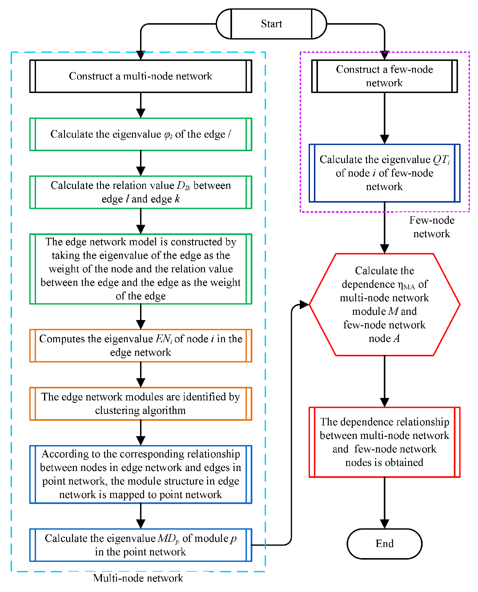
Figure 1. The method flow of this paper. The blue dotted box shows the calculation process of the multi-node network, and the purple dotted box shows the calculation process of the few-node network.
Systems 12 00433 g001
Figure 2. Common node extraction. Blue nodes are the endpoints of edges, green and purple nodes are the adjacent nodes of the blue nodes, and purple nodes are the common adjacent nodes of the endpoints of two edges.
Systems 12 00433 g002
Figure 3. The node-based network is transformed into an edge-based model. The network of blue nodes on the right is an edge network derived from the red-node network on the left. This edge network consists of 16 nodes, which correspond to the 16 edges in the node network. For example, the blue node “1–2” in the right diagram represents an edge mapped from vertices 1 and 2 in the node network on the left.
Systems 12 00433 g003
Figure 4. Network module relationship mapping. In the edge network on the left, nodes of the same color belong to the same module. When mapped to the node network, the module division of the nodes is shown in the diagram on the right. Nodes within the same module are indicated by curves of the same color. For example, the nodes within the red curve are mapped from the red nodes in the network on the left.
Systems 12 00433 g004
Figure 5. Few-node network.
Systems 12 00433 g005
Figure 6. Dependent edge prediction results. The upper layer is the few-node network, the lower layer is the multi-node network, the black dots represent the nodes of the network, the blue solid lines are the edges in the network, and the red dashed lines are the dependency edges between the two networks.
Systems 12 00433 g006
Figure 7. Power network model. (a) is an electrical diagram of the power network; (b) is a complex network model of the power network in (a).
Systems 12 00433 g007
Figure 8. Gas network model. (a) is the Belgian 20-node gas network; (b) is the network model of (a).
Systems 12 00433 g008
Figure 9. Edge-based model of the power grid.
Systems 12 00433 g009
Figure 10. Power–gas dependency network. The upper layer represents the natural gas network model, while the lower layer represents the power network model. The blue edges indicate the relationships between nodes within independent subnets, and the red dashed lines represent the interdependent edges predicted by this method.
Systems 12 00433 g010
Figure 11. Random edge situation: (a) the change process of natural connectivity index of three dependent networks under random edge attack; (b) the change process of geodesic vulnerability index of three dependent networks under random edge attack; (c) the change process of network efficiency index of three dependent networks under random edge attack. The red “TZ” represents the change curve of the homogeneous interdependent network model, the blue “YZ” represents the change curve of the heterogeneous interdependent network model, and the green “BW” represents the change curve of the modular interdependent network model obtained by the prediction method in this paper. The horizontal axis represents the number of edges removed, and the vertical axis represents the value of the network robustness evaluation metric.
Systems 12 00433 g011
Figure 12. High-betweenness edge attack situation. (a) The change process of natural connectivity index of three dependent networks under high-betweenness edge attack; (b) the change process of geodesic vulnerability index of three dependent networks under high-betweenness edge attack; (c) the change process of network efficiency index of three dependent networks under high-betweenness edge attack. The red “TZ” represents the change curve of the homogeneous interdependent network model, the blue “YZ” represents the change curve of the heterogeneous interdependent network model, and the green “BW” represents the change curve of the modular interdependent network model obtained by the prediction method in this paper. The horizontal axis represents the number of edges removed, and the vertical axis represents the value of the network robustness evaluation metric.
Systems 12 00433 g012
Figure 13. Course network.
Systems 12 00433 g013
Figure 14. Competency network model. CX is innovation competency, RD is software development Competency, XJ is system integration competency, MG is modeling competency, YD is hardware development competency, XG is project management competency, WJ is problem-solving competency.
Systems 12 00433 g014
Figure 15. Course edge-based model.
Systems 12 00433 g015
Figure 16. Course–competency dependency network.
Systems 12 00433 g016
Figure 17. Accuracy of course and competency target prediction. The horizontal axis in the figure is the course number in Table 7, and the red dashed line is the average prediction accuracy for all courses.
Systems 12 00433 g017
Figure 18. Accuracy of competency-supporting course prediction. CX is innovation competency, RD is software development competency, XJ is system integration competency, MG is model construction competency, YD is hardware development competency, XG is project management competency, WJ is problem-solving competency.
Systems 12 00433 g018
Figure 19. Text network model.
Systems 12 00433 g019
Figure 20. Add an edge to the network model.
Systems 12 00433 g020
Figure 21. Text edge-based model.
Systems 12 00433 g021
Figure 22. Text–question dependency network.
Systems 12 00433 g022
Figure 23. Information gain values of text and 30 problem-dependent words.
Systems 12 00433 g023
Table 1. Node-based network node attribute vectors.
NodeAttribute 1Attribute 2NodeAttribute 1Attribute 2
10.70.891.90.7
20.51.2101.10.5
320.8111.31.1
40.40.9121.61.9
50.51.3130.70.9
62.11.2140.71
70.80.9150.30.8
81.70.8162.11.8
Attribute 1 and Attribute 2 are the elements of the node attribute vectors.
Table 2. Edge-based model node weights.
NodeWeightsNodeWeightsNodeWeightsNodeWeights
1–20.474 3–120.706 5–150.100 9–100.898
1–60.662 6–50.542 4–130.291 11–120.493
2–30.210 6–80.399 7–80.552 11–140.774
2–50.800 6–160.982 7–90.265 13–140.599
3–40.645 5–70.187 8–100.700 15–160.613
Table 3. Nodes and characteristic values of each module.
ModuleNode in a ModuleCharacteristic Values
1Node 2, 3, 5, 6, 7, 8, 9, 10, 153.125
2Node 4, 11, 13, 142
3Node 16, 1, 2, 6, 83
4Node 3, 4, 9, 10, 11, 12, 15, 162.2
Table 4. Power network module division results.
ModuleNode Number in the ModuleAverage Degree Value
16, 137, 138, 139, 12, 140, 14, 15, 16, 17, 18, 19, 20, 21, 79, 80, 89, 90, 92, 94, 95, 98, 100, 103, 107, 58, 59, 608.011
27, 76, 77, 78, 104, 85, 86, 87, 24, 30, 37, 39, 40, 41, 42, 43, 44, 45, 46, 47, 48, 49, 50, 51, 52, 53, 54, 56, 57, 623.152
3128, 129, 130, 131, 133, 134, 135, 136, 9, 10, 11, 138, 139, 141, 142, 144, 143, 145, 32, 61, 63, 64, 65, 66, 67, 68, 69, 70, 71, 72, 73, 74, 75, 82, 91, 97, 101, 102, 108, 109, 112, 115, 116, 117, 118, 119, 120, 123, 125, 126, 12710.44
41, 2, 3, 4, 5, 6, 7, 9, 10, 11, 12, 13, 14, 15, 16, 17, 18, 19, 20, 21, 22, 27, 28, 29, 32, 33, 37, 39, 40, 45, 46, 54, 55, 56, 57, 58, 61, 62, 76, 83, 84, 86, 87, 88, 89, 93, 98, 100, 1034.977
57, 8, 12, 13, 25, 26, 27, 28, 29, 31, 58, 59, 60, 61, 63, 66, 68, 70, 71, 72, 73, 74, 75, 81, 82, 91, 95, 96, 98, 100, 101, 102, 103, 105, 106, 108, 109, 111, 112, 117, 135, 136, 137, 138, 139, 140, 1458.636
659, 63, 64, 65, 66, 67, 68, 69, 70, 71, 72, 73, 74, 75, 82, 91, 97, 101, 108, 109, 112, 116, 117, 118, 119, 120, 121, 122, 123, 124, 125, 127, 128, 129, 130, 131, 132, 133, 136, 141, 142, 143, 14414.224
734, 99, 36, 38, 881.833
82, 3, 4, 5, 6, 7, 8, 22, 23, 24, 30, 33, 34, 35, 37, 38, 39, 40, 43, 44, 45, 46, 47, 48, 49, 50, 53, 54, 55, 56, 57, 77, 78, 83, 87, 110, 113, 1145.016
Table 5. Dependent relationship prediction results xiugof Power-Gas Network.
The Dependence Relationship between Gas Network Nodes and Power Network Modules
Gas network nodeC 1F 2G 3K 4O 5P 6S 7T 8
Power network moduleModule6Module3Module5Module1Module8Module7Module4Module2
1 C is Brugge (3), 2 F is Antwepen (6), 3 G is Gent (7), 4 K is Liege (11), 5 O is Mons (15), 6 P is Blaregnies (16), 7 S is Arlon (19), 8 T is Petange (20).
Table 6. Power–gas network dependent edge prediction results.
TnetDnetTnetDnetTnetDnetTnetDnetTnetDnetTnetDnet
C67C144F116G137C132P99
C82F128F117G139C136S89
C91F130F118G140C141S93
C97F131F119G145C142S98
C101F134G60K137C143C131
C108F135G82K139S103F101
C109F136G91K140F102G109
C112F139G95K79F108O110
C116F141G96K80F109S100
C117F142G98K89F112C130
C118F144G100K90F115F97
C119F143G101K94T104G108
C121F145G102K95G111K60
C122F67G103K98G112G136
C124F82G105K100G117G135
C128F91G106K103
C is Brugge (3), F is Antwepen (6), G is Gent (7), K is Liege (11), O is Mons (15), P is Blaregnies (16), S is Arlon (19), T is Petange (20).
Table 7. Course names and their attribute vector values.
No.Course NameDUADAENo.Course NameDUADAE
1Digital Electronic Technology0.80.227Fundamentals of Computer Simulation0.50.5
2Analog Electronics Experiment0.60.428Sensor Technology0.60.4
3Digital Electronics Experiment0.60.429New Technology Topics0.20.8
4High-Frequency Electronic Technology0.90.130Wireless Sensor Networks0.50.5
5EDA Technology and Applications0.70.331Introduction to IoT0.30.7
6System-on-Chip Design0.50.532RF Identification Technology0.80.2
7Engineering Ethics1033FPGA Engineering Applications0.50.5
8Project Management0.90.134Programming Internship0.40.6
9Pattern Recognition and Applications0.90.135Production Internship0.20.8
10Physics0.60.436Computer Network Technology Internship0.30.7
11Circuit Theory0.80.237EDA Course Internship0.30.7
12Analog Electronic Technology0.80.238Comprehensive Professional Internship0.10.9
13Digital Electronics Internship0.40.639Graduation Internship0.50.5
14Electronic CAD Internship0.50.540Graduation Thesis0.30.7
15Electronic Circuit Internship0.60.441Microcontroller Principles and Interface Technology0.80.2
16Signals and Systems0.70.342Microcontroller Systems Internship0.50.5
17DSP Technology and Applications0.70.343Electronic Process Internship0.50.5
18DSP Course Internship0.30.744Electronic System Design0.60.4
19Communication Principles0.80.245Innovation and Quality Development Elective0.20.8
20Embedded Systems and Applications0.70.346Electronic Systems Internship0.20.8
21Embedded Systems Internship0.60.447Fundamentals of University Computing0.80.2
22Programming0.50.548Computer Programming0.50.5
23Computer Network Technology0.80.249Fundamentals of Microelectronic System Integration0.90.1
24Digital Signal Processing0.80.250Data Structures0.90.1
25Electromagnetic Fields and Waves0.70.351Image Processing Technology0.10.9
26RF Electronic Circuits0.70.352Basic Manufacturing Technology Internship0.50.5
Table 8. Structural attribute values of the edge-based model before and after optimization.
Number of NodesNumber of EdgesDensityAverage DegreeAverage BetweennessAverage BetweennessAverage Clustering Coefficient
Before356628730.995353.221.4170.9950.995
After349251320.4139144.020.00170.6450.755
Table 9. Course network module division results.
Capability NodeModuleNode Number in the ModuleAverage Degree Value
YD11, 5, 6, 7, 9, 10, 11, 12, 13, 14, 15, 17, 18, 19, 22, 23, 24, 26, 27, 28, 29, 31, 32, 33, 41, 42, 43, 45, 49, 5114.519
XJ121, 5, 6, 7, 11, 12, 14, 15, 16, 17, 19, 25, 26, 27, 28, 30, 31, 32, 33, 38, 39, 40, 42, 49, 5130.41
RD173, 4, 5, 9, 11, 14, 15, 16, 17, 18, 24, 25, 26, 28, 29, 33, 39, 41, 42, 43, 4913.688
XG52, 35, 34, 9, 44, 45, 46, 48, 227.357
CX91, 2, 4, 5, 6, 10, 11, 12, 13, 15, 16, 19, 21, 22, 25, 27, 28, 29, 30, 31, 32, 33, 34, 35, 37, 38, 39, 40, 44, 47, 48, 49, 51, 5219.53
WJ31, 3, 7, 8, 9, 10, 11, 12, 14, 16, 17, 18, 19, 20, 21, 22, 23, 24, 26, 27, 28, 29, 30, 31, 32, 35, 36, 37, 38, 39, 40, 41, 42, 43, 44, 45, 47, 49, 5124.134
MG152, 8, 10, 42, 44, 13, 45, 47, 50, 21, 23, 299.429
CX is innovation competency, RD is software development competency, XJ is system integration competency, MG is modeling competency, YD is hardware development competency, XG is project management competency, WJ is problem-solving competency.
Table 10. Text network module division results.
ModuleNode in the ModuleAverage Degree Value
1official, borders, share, team, ronaldo, countries, plays, martin, languages, genre, spain, border, uk, new, george, german, cristiano, york, speak, democracy, played5.2
2mary, bobby, wife, mexico, roger, die, battle, anne, sisters, flower, federer, hutchinson, called, state, christopher, texas, paris4.1
3died, king, adolf, school, james, government4.2
4vp, catholic, today, official, borders, greece, holy, type, simpson, matt, currency, married, speak, denmark, kids, new, college, people, language, share, city, play, played11.7
5writing, river, shot, zip, united, star, got, map, jordan, wars, chinese, francisco, states, kingdom, fox, darth, code, start, michael, ray, allen, vader, names, located, founded, milk, san, parents1.5
6year, harrison, frank, drafted, die, battle, henry, time, texas, antietam2.6
7greece, beckham, official, russia, college, johnny, government, depp, david, married, john, kind, today3.9
8president, justin, start, party, famous, county, shows, bieber, obama, instruments2.2
9use, republic, type, music, country, singapore, currency, john, australia, adolf, school, money, people, government, religion, speak, guitar, switzerland7.2
10university, president, died, led, political, split, party, james, die, located, form2.8
11use, team, ronaldo, type, george, cristiano, language, speak, guitar, currency, play, played16.8
12university, mary, school, movies, luther, king, high, martin3.8
13compose, year, style, garcia, music, plays, country, jerry, magellan, kind, come3.1
14died, mary, school, married, form, luther, government, ancient, hitler, egypt4.5
15cena, pope, new, famous, john, live, happened, state, adams5.7
16die, president, died, harrison, henry4.2
17turkey, official, borders, share, cook, republic, countries, currency, czech, john, used, guitar, work, dominican, people, speak, tim, switzerland, italy, kind7.5
18political, speakers, china, live, king, english, henry, luther, spain, distributed3.0
19paul, new, team, movies, ronaldo, george, people, cristiano, york, leader, married, australia, come4.0
20beckham, use, team, type, countries, music, country, currency, johnny, movies, people, language, depp, speak, david, play, come, kind, played13.7
Table 11. Dependent relationship prediction results.
Dependency Relationship between Competency Network Nodes and Course Network Modules
Problem Network Nodesrolesmoviescountriestheiractorsplayed
Text Network ModulesModule 28Module 11Module 1Module 5Module 30Module 25
Disclaimer/Publisher’s Note: The statements, opinions and data contained in all publications are solely those of the individual author(s) and contributor(s) and not of MDPI and/or the editor(s). MDPI and/or the editor(s) disclaim responsibility for any injury to people or property resulting from any ideas, methods, instructions or products referred to in the content.