Article

Prediagnosis of Disease Based on Symptoms by Generalized Dual Hesitant Hexagonal Fuzzy Multi-Criteria Decision-Making Techniques

by
Alaa Fouad Momena
1,*,
Shubhendu Mandal
2,
Kamal Hossain Gazi
3,
Bibhas Chandra Giri
2 and
Sankar Prasad Mondal
3
1
Department of Industrial Engineering, College of Engineering, Prince Sattam Bin Abdulaziz University, Al Kharj 11942, Saudi Arabia
2
Department of Mathematics, Jadavpur University, Kolkata 700032, West Bengal, India
3
Department of Applied Mathematics, Maulana Abul Kalam Azad University of Technology, Kalyani 741249, West Bengal, India
*
Author to whom correspondence should be addressed.
Systems 2023, 11(5), 231; https://doi.org/10.3390/systems11050231
Submission received: 28 March 2023 / Revised: 25 April 2023 / Accepted: 28 April 2023 / Published: 6 May 2023

Abstract

:
Multi-criteria decision-making (MCDM) is now frequently utilized to solve difficulties in everyday life. It is challenging to rank possibilities from a set of options since this process depends on so many conflicting criteria. The current study focuses on recognizing symptoms of illness and then using an MCDM diagnosis to determine the potential disease. The following symptoms are considered in this study: fever, body aches, fatigue, chills, shortness of breath (SOB), nausea, vomiting, and diarrhea. This study shows how the generalised dual hesitant hexagonal fuzzy number ( G D H H χ F N ) is used to diagnose disease. We also introduce a new de-fuzzification method for G D H H χ F N . To diagnose a given condition, G D H H χ F N coupled with MCDM tools, such as the fuzzy criteria importance through inter-criteria correlation (FCRITIC) method, is used for finding the weight of criteria. Furthermore, the fuzzy weighted aggregated sum product assessment (FWASPAS) method and a fuzzy combined compromise solution (FCoCoSo) are used to rank the alternatives. The alternative diseases are chosen to be malaria, influenza, typhoid, dengue, monkeypox, ebola, and pneumonia. A sensitivity analysis is carried out on three patients affected by different diseases to assess the validity and reliability of our methodologies.

1. Introduction

The maximum value of the degree of belongingness in fuzzy sets is 1. Suppose more than one decision-maker is participating in the same context when making a qualitative judgment. This maximum degree of membership may differ from one decision-maker to the other. Thus, the generalized fuzzy number was introduced [1]. The idea behind generalized fuzzy numbers is to extend the concept of fuzzy numbers beyond their traditional triangular or trapezoidal shapes. Generalized fuzzy numbers allow for more flexible shapes, which can better capture the uncertainty or imprecision inherent in many real-world situations. Generalized fuzzy numbers have been widely used in fuzzy mathematics [2,3,4], decision-making [5,6], and control theory [7], among other fields [2,8,9]. They provide a useful tool for representing uncertain or vague information in a formal way and for making decisions in situations where there is a high degree of uncertainty or ambiguity. Hesitant fuzzy sets ( H F S ) can be used to recognize diseases by allowing the degree of membership of an element to multiple possible sets or categories to be expressed as a range of values rather than a single crisp value. This is particularly useful in medical diagnosis [10], where there may be a degree of uncertainty or ambiguity in assigning a patient to a particular disease category based on their symptoms or test results. This method can be used to model the uncertainty and imprecision inherent in medical diagnosis by allowing the degree of membership of an element to be expressed as a range of values between 0 and 1. This makes it possible to make decisions that are more flexible and nuanced, which can help to reduce the risk of misdiagnosis. Overall, hesitant fuzzy sets can be a valuable tool for recognizing diseases, particularly in situations where there is a high degree of uncertainty or ambiguity in the diagnosis process. Liao, H. et al. [11] proposed qualitative decision-making with correlation coefficients of hesitant fuzzy linguistic term sets in medical diagnosis. Mardani, A. et al. [12] introduced a novel extended approach using hesitant fuzzy sets to design a framework for assessing the key challenges of digital health intervention adoption during the COVID-19 pandemic. Ghorui, N. et al. [13] identified the dominant risk factor involved in the spread of COVID-19 using hesitant fuzzy MCDM methodology. In addition to medical diagnosis, a great deal of study in other areas [14,15] involving hesitant fuzzy sets has been carried out. Additionally, many studies have been conducted on generalized fuzzy numbers, including generalized triangular intuitionistic fuzzy numbers ( G T I F N ) [16], generalized trapezoidal hesitant fuzzy numbers ( G T r H F N ) [2], generalized hesitant fuzzy numbers ( G H F N ) [8], and generalized hexagonal fuzzy numbers ( G H χ F N ) [17]. However, as far as we know, there is currently no research on the use of a generalized dual hesitant hexagonal fuzzy ( G D H H χ F ) MCDM technique for disease recognition. Hence, in this paper, we focus on this issue and use specific MCDM techniques, such as fuzzy criteria importance through inter-criteria correlation (FCRITIC), fuzzy weighted aggregated sum product assessment (FWASPAS), and fuzzy combined compromise solution (FCoCoSo), to recognize a patient’s disease using a new fuzzy environment called a generalized dual hesitant hexagonal fuzzy number ( G D H H χ F N ).
The generalized dual hesitant hexagonal fuzzy multi-criteria decision-making ( G D H H χ F -MCDM) technique can be used to recognize diseases by considering multiple criteria and factors that may affect the diagnosis process. The first step in using the G D H H χ F -MCDM technique for disease recognition is to identify the relevant criteria and factors that are associated with the disease. These criteria may include medical symptoms, patient history, laboratory results, imaging tests, and other diagnostic tools. Next, the experts or decision-maker in the field can assign weights to each criterion based on its importance in the disease recognition process. These weights can be determined using professional judgment, statistical analysis, or other methods. Then, the experts can use the G D H H χ F -MCDM methods to evaluate each criterion based on its linguistic variable and their degree of membership and non-membership values. This technique allows for the use of dual hesitant fuzzy numbers, which can represent uncertainty and vagueness in the evaluation process. Finally, the G D H H χ F -MCDM technique can be used to aggregate the evaluations of each criterion and provide an overall diagnosis of the disease. The technique can also be used to rank the potential diseases of a patient based on their likelihood of being the correct diagnosis.
Overall, the G D H H χ F -MCDM technique can help to improve the accuracy and efficiency of disease recognition by considering multiple criteria and sub-criteria in the decision-making process.

1.1. Motivation of the Study

There need to be more suitable decision mechanisms in the context of current studies relating to disease-recognizing issues. The multiple-criteria decision-making (MCDM) methods have used numerous successful real-world challenges to examine difficult decisions and appropriately make a proper decision. To address the vital characteristic aspects that match integrating MCDM and the diseases recognition problem, further research into the emergence of MCDM in addressing the diseases recognition problem is required. On the other hand, if uncertainties are with the whole situation, then the problem is more complex to solve. Hesitant fuzzy ideology is one of the preferable uncertainties for the diagnosis problem. This study will provide MCDM, fuzzy sets theory, and its extensions to researchers and the broader community for tackling an accurate decision for disease diagnosis problems.

1.2. Research Outline

Based on the above introduction and especially research motivation, the primary outlines of this paper are as follows:
  • For pre-diagnosis of the diseases, pick the disorders that are caused by viruses, have many overlapping symptoms, and have been scientifically identified.
  • Identifying the symptoms of different diseases and comparative studies on signs with slight differences.
  • Develop a comparative matrix based on criteria and alternatives for the Generalized Dual Hesitant Hexagonal fuzzy number ( G D H H x F N ) by the decision-makers (DMs) to capture all the ambiguity, hesitancy, and vagueness.
  • Calculate the criteria weight using the MCDM method FCRITIC. According to decision experts, this part identifies which symptoms are more severe and dangerous than others.
  • Rank the diseases by FWASPAS and FCoCoSo, two MCDM methods for pre-diagnosis and early treatment. The two approaches mentioned above are considered concurrently for robustness and to ensure the consistency of our ranking.
  • We conducted sensitivity and comparative analyses to check the result’s vagueness and unbiasedness. It demonstrates that how internally consistent our results are.

1.3. Structure of the Paper

Section 1 contains the introduction and motivation for this study. The literature review on methodology and applications are covered in Section 2. Then, Section 3 and Section 4 include preliminaries of mathematical tools and MCDM methodology, respectively. Then the alternatives are discussed in Section 5. Section 6 described the symptoms of the disease and model setup. Next, data collection and numerical description are covered in Section 7 and Section 8, respectively. Sensitivity analysis and Comparative analysis are described in Section 9. Section 10 discuss practical implication. Finally, the conclusion and future research extension are contained in Section 11.

2. Literature Review

This section introduces the necessary basic key terms and their recent uses. Disease recognition is crucial in healthcare domains, and MCDM supports decision-making. MCDM is a decision-making technique considering multiple criteria and a weighted combination of these criteria from various alternatives. The literature on disease recognition using MCDM covers numerous aspects, including the application of MCDM in medical decision-making, the development of novel MCDM models for disease recognition, and the evaluation of the effectiveness of these models. Several studies have used MCDM to develop decision support systems for various diseases in Table 1 and Table 2. Moreover, Table 3 and Table 4 cover recent work on dual hesitant fuzzy numbers and generalized fuzzy numbers, respectively.

3. Preliminaries

This section apprises the basic definitions relating to fuzzy sets (FS), membership function, generalization of FS, hesitation of FS, and some algebraic operations which will be needed to elucidate the scope of this paper.

3.1. Fuzzy Set Theory

Prof. Lotfi A. Zadeh presented fuzzy sets [74] from the University of California at Berkeley in 1965. A fuzzy set is a set that is characterized by a membership function (MF). Qualitative and subjective viewpoints are communicated by linguistic variables, which are quantitatively expressed by a fuzzy set in the context of discourse and the corresponding MF [75,76]. The fuzzy set represents impreciseness, fully intent on decreasing intricacy by disposing of the sharp limit isolating the members from the pair from non-members. Every component in this set with its degree of membership value [77]. The definition of the fuzzy set and its membership function is described below. There exist different MCDM problems associated with an extension of the fuzzy set, such as interval-valued fuzzy soft set [78] and the interval-valued intuitionistic fuzzy set [79].

3.1.1. Generalized Fuzzy Number

A generalized fuzzy number A ˜ = ( ξ a , ξ b , ξ c , ξ d , ξ e , ξ f ; Ω ˜ ) is described as any fuzzy set (especially, A ˜ be a generalized hexagonal fuzzy number, more details are later) of the real line R with membership function μ A ˜ that possesses the following features:
1.
μ A ˜ ( y ) : R [ 0 , Ω ˜ ] is continuous, Ω ˜ ( 0 , 1 ] ,
2.
μ A ˜ ( y ) = 0 for all y ( , ξ a ) ,
3.
μ A ˜ ( y ) is monotonically increasing on [ ξ a , ξ b ) and [ ξ b , ξ c ) ,
4.
μ A ˜ ( y ) = ω ˜ for all y [ ξ c , ξ d ] ,
5.
μ A ˜ ( y ) is monotonically decreasing on ( ξ d , ξ e ] and ( ξ e , ξ f ] ,
6.
μ A ˜ ( y ) = 0 for all y ( ξ f , ) .

3.1.2. Hesitant Fuzzy Number

Torra, V. et al. [80] put out a notion known as the hesitant fuzzy set (HFS). When a decision-maker is not entirely satisfied with a precise membership degree, HFSs can address the intrinsic ambiguity in the decision-making process by enabling the decision-maker to describe their preference with a membership function containing a greater variety of values [81]. Chen, N. et al. [82] also discussed HFS. When compromised decisions are used in group decision-making challenges, HFSs are preferred more. Torra, V. et al. [80] represented the HFS as follows:
Definition 1.
Assume Y ϑ be a fixed set. Hesitant fuzzy set (HFS) F ˜ ε h is defined on Y ϑ to [ 0 , 1 ] . The HFS is represented as follows,
F ˜ ε h = ( < y , μ F ˜ ε h ( y ) > | y Y ϑ )
where μ F ˜ ε h ( y ) denotes the possible membership function of the set F ˜ ε h , bounded by [ 0 , 1 ] . For convenience, μ F ˜ ε h = μ F ˜ ε h ( y ) is called a hesitant fuzzy element (HFE).

3.1.3. Dual Hesitant Fuzzy Number

Zhu, B. et al. [83] defined the dual hesitant fuzzy number (DHFN). Tyagi, S.K. [84] also discusses it. DHFN are defined as follows:
Definition 2.
Suppose there is a fixed set Y ϑ . A DHFS D ˜ ε h on the fixed set Y ϑ is described as follows,
D ˜ ε h = { < y , μ D ˜ ε h ( y ) , ν D ˜ ε h ( y ) > | y Y ϑ }
where μ D ˜ ε h ( y ) and ν D ˜ ε h ( y ) are the membership and non-membership degree, respectively, and satisfies the following conditions:
(a).
0 μ D ˜ ε h , ν D ˜ ε h 1 for all y Y ϑ
(b).
0 μ D ˜ ε h + + ν D ˜ ε h 1 where μ D ˜ ε h + = max y Y ϑ { ν D ˜ ε h ( y ) } and ν D ˜ ε h = max y Y ϑ { ν D ˜ ε h ( y ) }

3.1.4. Basic Operation of DHFS

Consider two DHFS Δ ˜ ε h , Γ ˜ ε h on Y ϑ and described as Δ ˜ ε h = { < ξ , μ Δ ˜ ε h ( ξ ) , ν Δ ˜ ε h ( ξ ) > | ξ Y ϑ } and Γ ˜ ε h = { < ξ , μ Γ ˜ ε h ( ξ ) , ν Γ ˜ ε h ( ξ ) > | ξ Y ϑ } . Then, some basic set operations and arithmetic operations on them are defined as follows:
A.
Complement of Δ ˜ ε h
Δ ˜ ε h c = { < ξ , ν Δ ˜ ε h ( ξ ) , μ Δ ˜ ε h ( ξ ) > | ξ Y ϑ }
B.
Union of Δ ˜ ε h and Γ ˜ ε h
Δ ˜ ε h Γ ˜ ε h = μ Δ ˜ ε h Δ ˜ ε h , μ Γ ˜ ε h Γ ˜ ε h , ν Δ ˜ ε h Δ ˜ ε h , ν Γ ˜ ε h Γ ˜ ε h < ξ , max { μ Δ ˜ ε h ( ξ ) , μ Γ ˜ ε h ( ξ ) } , min { ν Δ ˜ ε h ( ξ ) , ν Γ ˜ ε h ( ξ ) } > | ξ Y ϑ
C.
Intersection of Δ ˜ ε h and Γ ˜ ε h
Δ ˜ ε h Γ ˜ ε h = μ Δ ˜ ε h Δ ˜ ε h , μ Γ ˜ ε h Γ ˜ ε h , ν Δ ˜ ε h Δ ˜ ε h , ν Γ ˜ ε h Γ ˜ ε h < ξ , min { μ Δ ˜ ε h ( ξ ) , μ Γ ˜ ε h ( ξ ) } , max { ν Δ ˜ ε h ( ξ ) , ν Γ ˜ ε h ( ξ ) } > | ξ Y ϑ
D.
Addition of Δ ˜ ε h and Γ ˜ ε h
Δ ˜ ε h Γ ˜ ε h = μ Δ ˜ ε h Δ ˜ ε h , μ Γ ˜ ε h Γ ˜ ε h , ν Δ ˜ ε h Δ ˜ ε h , ν Γ ˜ ε h Γ ˜ ε h < ξ , ( μ Δ ˜ ε h ( ξ ) + μ Γ ˜ ε h ( ξ ) μ Δ ˜ ε h ( ξ ) μ Γ ˜ ε h ( ξ ) ) , ( ν Δ ˜ ε h ( ξ ) ν Γ ˜ ε h ( ξ ) ) > | ξ Y ϑ
E.
Multiplication of Δ ˜ ε h and Γ ˜ ε h
Δ ˜ ε h Γ ˜ ε h = μ Δ ˜ ε h Δ ˜ ε h , μ Γ ˜ ε h Γ ˜ ε h , ν Δ ˜ ε h Δ ˜ ε h , ν Γ ˜ ε h Γ ˜ ε h < ξ , ( μ Δ ˜ ε h ( ξ ) μ Γ ˜ ε h ( ξ ) ) , ( ν Δ ˜ ε h ( ξ ) + ν Γ ˜ ε h ( ξ ) ν Δ ˜ ε h ( ξ ) ν Γ ˜ ε h ( ξ ) ) > | ξ Y ϑ

3.2. Hexagonal Fuzzy Number ( H χ F N )

Definition 3.
[85,86] Let Y ϑ be the fixed set and ξ p , ξ q , ξ r , ξ s , ξ t , ξ u R , such that ξ p ξ q ξ r ξ s ξ t ξ u . Then, a hexagonal fuzzy number ψ N on Y ϑ is defined as
ψ N = < ( ξ p , ξ q , ξ r , ξ s , ξ t , ξ u ) : α , 1 > = < ( ξ p , ξ q , ξ r , ξ s , ξ t , ξ u ) : α >
with membership function μ ψ N defined as
μ ψ N ( y ) = 0 if y < ξ p α y ξ p ξ q ξ p i f ξ p y < ξ q α + ( 1 α ) y ξ q ξ r ξ q i f ξ q y < ξ r 1 i f ξ r y ξ s α + ( 1 α ) y ξ t ξ s ξ t i f ξ s < y ξ t α y ξ μ ξ t ξ μ i f ξ t < y ξ μ 0 i f ξ μ < y
where y R and α [ 0 , 1 ] .
Note 1.
The range of α is [ 0 , 1 ] and if
  • α = 0 then hexagonal fuzzy number ψ N becomes trapezoidal fuzzy number
    ψ = < ( ξ q , ξ r , ξ s , ξ t ) > .
  • α = 1 then hexagonal fuzzy number ψ N becomes trapezoidal fuzzy number
    ψ = < ( ξ p , ξ q , ξ t , ξ u ) > .
  • α ( 0 , 1 ) then hexagonal fuzzy numbers ψ N are not restructured.
Therefore, in general, always consider α ( 0 , 1 ) .
Figure 1 describes the structural representation of the membership function of H χ F N , where α lies in ( 0 , 1 ) and the highest membership value is 1.

3.2.1. Arithmetic Operation on H χ F N

Let U = ( u 1 , u 2 , u 3 , u 4 , u 5 , u 6 ) and V = ( v 1 , v 2 , v 3 , v 4 , v 5 , v 6 ) be two H χ F N , then their general arithmetic operation can be defined in the following way:
1.
Addition:
U V = ( u 1 + v 1 , u 2 + v 2 , u 3 + v 3 , u 4 + v 4 , u 5 + v 5 , u 6 + v 6 )
2.
Subtraction:
U V = ( u 1 v 6 , u 2 v 5 , u 3 v 4 , u 4 v 3 , u 5 v 2 , u 6 v 1 )
3.
Multiplication:
U V = ( u 1 v 1 , u 2 v 2 , u 3 v 3 , u 4 v 4 , u 5 v 5 , u 6 v 6 )
4.
Scalar Multiplication:
α U = ( α u 1 , α u 2 , α u 3 , α u 4 , α u 5 , α u 6 )
5.
Division:
U V = U V = u 1 v 6 , u 2 v 5 , u 3 v 4 , u 4 v 3 , u 5 v 2 , u 6 v 1
6.
Inverse:
U 1 = 1 U = 1 u 6 , 1 u 5 , 1 u 4 , 1 u 3 , 1 u 2 , 1 u 1

3.2.2. Generalised Hexagonal Fuzzy Set

Definition 4.
[87] Let Y ϑ be the fixed set and ξ p , ξ q , ξ r , ξ s , ξ t , ξ u R such that ξ p ξ q ξ r ξ s ξ t ξ u . Then, a generalised hexagonal fuzzy set ψ g on Y ϑ is defined as:
ψ g = < ( ξ p , ξ q , ξ r , ξ s , ξ t , ξ u ) : α , β >
with membership function μ ψ g defined as
μ ψ N ( y ) = 0 if y < ξ p α y ξ p ξ q ξ p i f ξ p y < ξ q α + ( β α ) y ξ q ξ r ξ q i f ξ q y < ξ r β i f ξ r y ξ s α + ( β α ) y ξ t ξ s ξ t i f ξ s < y ξ t α y ξ μ ξ t ξ μ i f ξ t < y ξ μ 0 i f ξ μ < y
where y R and α , β [ 0 , 1 ] with α β .
Note 2.
Depending on the range and relation between α a n d β , the generalised hexagonal fuzzy set ( G H χ F S ) ψ g is restructured. The range is 0 α β 1 . Then, depending on the relation α a n d β , reshape the G H χ F S ψ g in the following way:
  • If α = β = 0 then the G H χ F S ψ g becomes a zero set.
  • If α = 0 and β ( 0 , 1 ) then the G H χ F S ψ g becomes generalised trapezoidal fuzzy set ψ = < ( ξ q , ξ r , ξ s , ξ t ) : β > .
  • If α = 0 and β = 1 then the G H χ F S ψ g becomes trapezoidal fuzzy set ψ = < ( ξ q , ξ r , ξ s , ξ t ) > .
  • If α ( 0 , 1 ) and β ( 0 , 1 ) with α < β then the G H χ F S ψ g unchanged.
  • If α ( 0 , 1 ) and β ( 0 , 1 ) with α = β then the G H χ F S ψ g becomes generalised trapezoidal fuzzy set ψ = < ( ξ p , ξ q , ξ t , ξ u ) : α > .
  • If α ( 0 , 1 ) and β = 1 then the G H χ F S ψ g becomes hexagonal fuzzy set
    ψ = < ( ξ p , ξ q , ξ r , ξ s , ξ t , ξ u ) : α > .
  • If α = β = 1 then the G H χ F S ψ g becomes trapezoidal fuzzy set ψ = < ( ξ p , ξ q , ξ t , ξ u ) > .
Figure 2 represented the generalised hexagonal fuzzy number ψ g = < ( ξ p , ξ q , ξ r , ξ s , ξ t , ξ u ) : α , β > . The highest membership value of ψ g is β and the value of α are in between 0 and β .

3.3. Generalized Hexagonal Dual Hesitant Fuzzy Set

A Hexagonal Dual Hesitant Fuzzy Set ( H χ D H F S ) is a hesitant fuzzy set introduced as an extension of the dual hesitant fuzzy set.

3.3.1. Hexagonal Dual Hesitant Fuzzy Set

Definition 5.
Let Y ϑ be a fixed set. Hexagonal dual hesitant fuzzy set ( H χ D H F S ) D ε h χ on Y ϑ is described as,
D ε h χ = { < y , ( μ ε h χ ( y ) , ν ε h χ ( y ) ) > | y Y ϑ }
where μ ε h χ ( y ) is the set of HFN possible membership values and ν ε h χ ( y ) is the set of HFN possible non-membership values of the element y Y ϑ to the set D ε h χ .

3.3.2. Hexagonal Dual Hesitant Fuzzy Number ( H χ D H F N )

If H χ F h ( y ) = { ( ξ p , ξ q , ξ r , ξ s , ξ t , ξ u ) | { μ ( y ) , ν ( y ) } } then H χ F h ( y ) is called the Hexagonal Dual Hesitant Fuzzy Element.

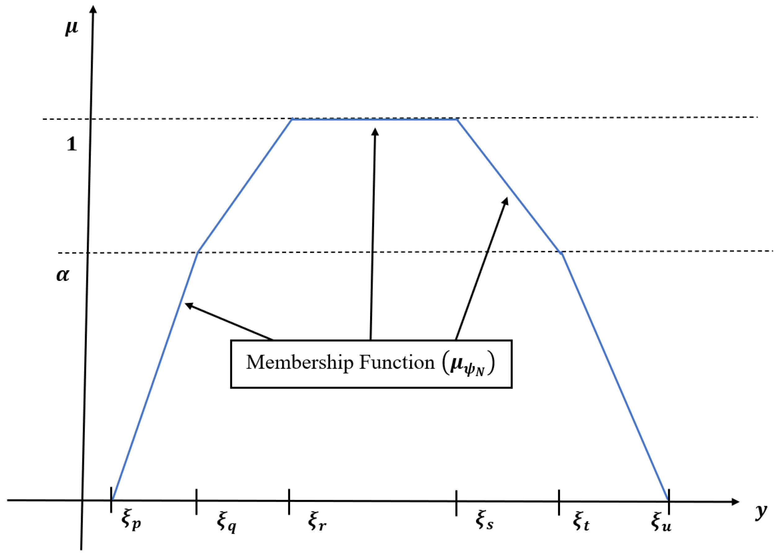
3.3.3. Generalized Hesitant Fuzzy Number ( G H F N )

It is a collection of generalized fuzzy numbers reflecting various membership functions that could be applied to the element y Y ϑ in the set of real numbers R . The generalized triangular hesitant fuzzy number ( G T H F N ) , generalized trapezoidal hesitant fuzzy number ( G T r H F N ) , and generalized pentagonal hesitant fuzzy numbers ( G P H F N ) are some examples of this form.

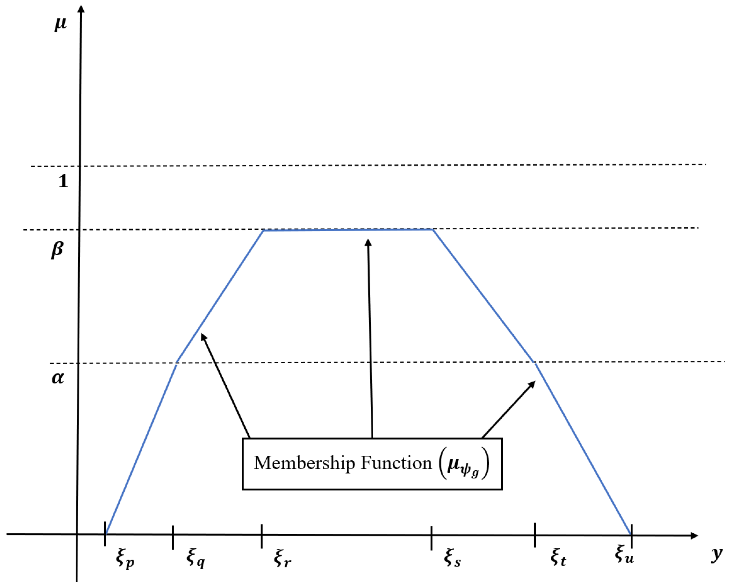
3.3.4. Generalized Hexagonal Fuzzy Number ( G H χ F N )

Generally, the maximum membership value of any fuzzy number is 1, but it needs not be the same for G H χ F N . Any values from ( 0 , 1 ] are acceptable. The G H χ F N is changed to H χ F N if the maximum membership value is 1.

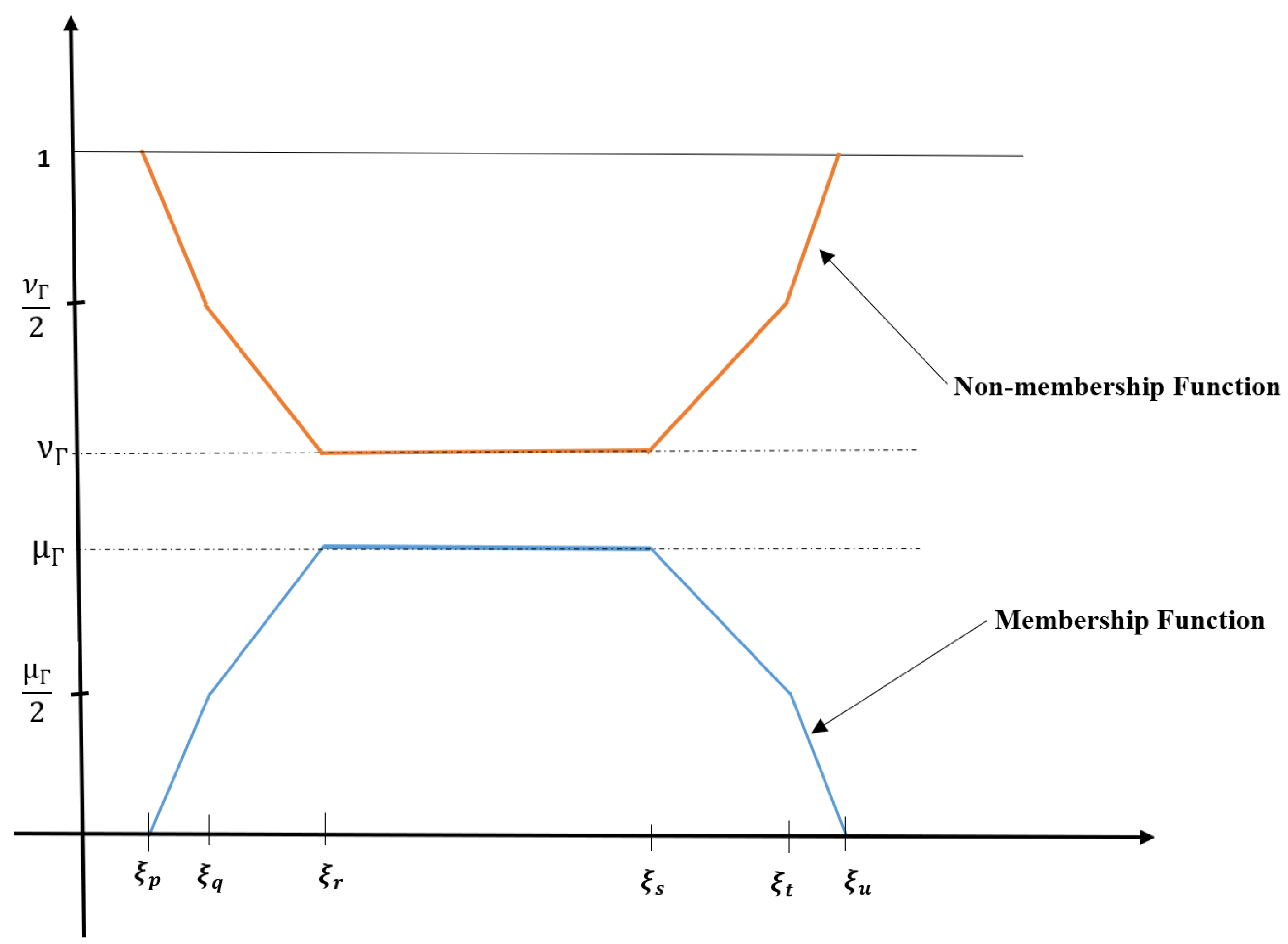
3.4. Generalized Dual Hesitant Hexagonal Fuzzy Number ( G D H H χ F N )

A G D H H χ F N is defined in this paper in two forms. In G D H H χ F N (1st type), the number of H χ F N can be more than one, but the number of membership and non-membership functions is restricted to one. In G D H H χ F N (2nd type), the number of the H χ F N is restricted to one, but the membership and non-membership functions can be more than one.

3.4.1. Benefits of D H F S Rather than  F S

A fuzzy set variation, known as the dual hesitant fuzzy set ( D H F S ), enables a more sophisticated representation of uncertainty and ambiguity. In contrast to fuzzy sets, which only allow partial membership of an element in a set, DHFS leads to a more fine-grained representation of uncertainty by allowing an element to be neither entirely in nor fully out of a set. Here are some benefits of DHFS over fuzzy sets:
(A)
D H F S may represent membership degrees that are positive or negative, whereas fuzzy sets can only do so for positive membership degrees. This makes it possible for D H F S to represent scenarios when one element is uncertain and potentially not a set member.
(B)
The uncertainty and hesitancy of a decision-maker can be better captured by D H F S than F S , producing more precise and dependable outcomes.
(C)
Decision-makers can make better decisions with access to more complete and accurate information from D H F S .
(D)
When handling uncertain or missing data, D H F S delivers additional flexibility, which can result in more reliable and adaptable decision-making systems.

3.4.2. Benefits of G D H H χ F S Rather than  F S

Somebody can use further development of the dual hesitant fuzzy set, the generalized dual hesitant hexagonal fuzzy set ( G D H H χ F S ), to communicate uncertainty more elaborately than fuzzy sets. The advantages of G D H H χ F S over fuzzy sets are as follows:
(a)
G D H H χ F S provides a more accurate and improved representation of uncertainty and ambiguous information than fuzzy sets. It can also represent the degree of hesitation in decision-making.
(b)
For handling ambiguous or missing data, G D H H χ F S provides greater flexibility. Under a single framework, it enables the representation of several kinds of uncertainty, including randomness, fuzziness, and incompleteness.
(c)
G D H H χ F S provides a clear and intuitive interpretation of each element’s membership and non-membership degrees, making it easy for decision-makers to understand and use and allowing for more informed and reliable decision-making.
Now we are focusing on G D H H χ F N .
Definition 6.
(Generalised Dual Hesitant Hexagonal Fuzzy Number G D H H χ F N ). Assume Y ϑ to be a fixed set, i ( T N ) be an integer and ξ p i , ξ q i , ξ r i , ξ s i , ξ t i , ξ u i R , such that the relation among them are ξ p i ξ q i ξ r i ξ s i ξ t i ξ u i , for all i T . Then generalised dual hesitant hexagonal fuzzy number G D H H χ F N is defined as
ψ = i T ( ξ p i , ξ q i , ξ r i , ξ s i , ξ t i , ξ u i ) ; μ ψ , ν ψ : i T
where μ ψ and ν ψ denotes the membership function and non-membership function, respectively.
Remark 1.
A generalized dual hesitant hexagonal fuzzy number is a collection of hexagonal fuzzy numbers with i T N . Additionally, G D H H χ F N can be formed by generalized fuzzy numbers, hesitant fuzzy numbers, dual hesitant fuzzy numbers, and hexagonal fuzzy numbers, as depicted in Figure 3.
We construct two forms of generalized dual hesitant hexagonal fuzzy numbers from the above definitions. In the first type of G D H H χ F N , the membership and non-membership functions are fixed, but the H χ F N can vary. In the second type, the H χ F N are considered to be fixed, but the membership and non-membership function for a specific H χ F N can differ depending on the preference of DMs.
Definition 7.
Let ψ = y , i T ( ξ p i , ξ q i , ξ r i , ξ s i , ξ t i , ξ u i ) : μ i , ν i : i T ; y Y ϑ represents a set of different G D H H χ F N . If μ i = μ for all i T then G D H H χ F N is reduced to a single membership function for different G D H H χ F N . Similarly, for non-membership function ν i = ν for all i T . This form of G D H H χ F N is said to be G D H H χ F N of the 1st type. It is structurally expressed in the following way
ψ G D H H χ F N 1 = y , i T ( ξ p i , ξ q i , ξ r i , ξ s i , ξ t i , ξ u i ) ; { μ , ν } : i T , y Y ϑ
The example of G D H H χ F N of the first type is presented in Example 1. Here, consider i = 2 and obtain two sets of H χ F N .
Example 1.
Consider ψ a 1 where a = 1 , 2 , , 6 are the G D H H χ F N of first type and represented as follows:
  • ψ 1 1 = < ( 5.3 , 5.4 , 5.6 , 5.7 , 5.8 , 5.9 ) , ( 5.4 , 5.5 , 5.6 , 5.8 , 5.9 , 6 ) ; { 0.9 , 0.1 } >
  • ψ 2 1 = < ( 4.4 , 4.5 , 4.7 , 4.8 , 4.9 , 5 ) , ( 4.8 , 4.9 , 5.1 , 5.2 , 5.3 , 5.4 ) ; { 0.8 , 0.1 } >
  • ψ 3 1 = < ( 3.8 , 4.9 , 4 , 4.1 , 4.2 , 4.3 ) , ( 4.5 , 4.6 , 4.7 , 4.8 , 4.9 , 5 ) ; { 0.7 , 0.2 } >
  • ψ 4 1 = < ( 3 , 3.1 , 3.2 , 3.4 , 3.5 , 3.6 ) , ( 3.4 , 3.5 , 3.6 , 3.7 , 3.8 , 4 ) ; { 0.5 , 0.4 } >
  • ψ 5 1 = < ( 2 , 2.2 , 2.3 , 2.4 , 2.5 , 2.6 ) , ( 2.4 , 2.5 , 2.6 , 2.7 , 2.8 , 2.9 ) ; { 0.3 , 0.6 } >
  • ψ 6 1 = < ( 1 , 1.2 , 1.3 , 1.4 , 1.5 , 1.6 ) , ( 1.3 , 1.4 , 1.5 , 1.6 , 1.7 , 1.9 ) ; { 0.2 , 0.5 } >
Remark 2.
G D H H χ F N can be used to describe the hesitancy or vagueness of a DM or group of DMs in different possible ways. Unlike the Generalized Dual Hesitant Triangular Fuzzy Number (GDHTFN), Generalized Dual Hesitant Trapezoidal Fuzzy Number (GDHTrFN), or Generalized Dual Hesitant Pentagonal Fuzzy Number (GDHPFN), which represents the impreciseness in three numbers, or four numbers or five numbers, respectively, G D H H χ F N considers six numbers and, thus, captures the uncertainty in better form.
Definition 8.
Let Γ = { < y , i T ( ξ p i , ξ q i , ξ r i , ξ s i , ξ t i , ξ u i ) ; μ Γ i , ν Γ i : i T > : y Y ϑ } represents a set of different G D H H χ F N . If ξ p = ξ p i , ξ q = ξ q i , ξ r = ξ r i , ξ s = ξ s i , ξ t = ξ t i , ξ u = ξ u i for all i T , G D H H χ F N is reduced to single valued generalized dual hesitant hexagonal fuzzy number with different set of membership and non-membership value. This form of G D H H χ F N is said to be the second type. Structurally expressed as
Γ G D H H χ F N 2 = y , ( ξ p , ξ q , ξ r , ξ s , ξ t , ξ u ) ; { ( μ Γ i , ν Γ i ) : μ Γ i μ Γ , ν Γ i ν Γ ; i T } : y Y ϑ
where μ Γ i ( [ 0 , 1 ] ) represent the membership value and ν Γ i ( [ 0 , 1 ] ) represent the non-membership value for every i T and y Y ϑ .
Definition 8 is a special form of dual hesitant fuzzy set on the set of real number R . The membership and non-membership functions of G D H H χ F N [88] are defined as follows:
{ μ Γ i ( y ) , ν Γ i ( y ) } = { 0 , 1 } if y < ξ p μ Γ 2 y ξ p ξ q ξ p , ν Γ 2 + 1 ν Γ 2 y ξ q ξ p ξ q if ξ p y < ξ q μ Γ 2 + 1 μ Γ 2 y ξ q ξ r ξ q , ν Γ 2 + ν Γ 2 y ξ q ξ r ξ q if ξ q y < ξ r { μ Γ , ν Γ } if ξ r y ξ s μ Γ 2 + 1 μ Γ 2 y ξ t ξ s ξ t , ν Γ 2 + ν Γ 2 y ξ t ξ s ξ t if ξ s < y ξ t μ Γ 2 y ξ μ ξ t ξ μ , ν Γ 2 + 1 ν Γ 2 y ξ t ξ μ ξ t if ξ t < y ξ μ { 0 , 1 } if ξ μ < y
Geometric representation of membership and non-membership functions of G D H H χ F N are displayed in Figure 4.
Example 2.
Numerically G D H H χ F N (2nd type) are shown as:
  • Γ ˜ 1 2 = < ( 8 , 8.5 , 9 , 10 , 10.5 , 11 ) ; { ( 0.70 , 0.15 ) , ( 0.75 , 0.20 ) , ( 0.65 , 0.20 ) } >
  • Γ ˜ 2 2 = < ( 7 , 7.5 , 8 , 9 , 9.5 , 10 ) ; { ( 0.65 , 0.15 ) , ( 0.85 , 0.05 ) , ( 0.75 , 0.10 ) } >
  • Γ ˜ 3 2 = < ( 6 , 6.5 , 7 , 8 , 8.5 , 9 ) ; { ( 0.80 , 0.10 ) , ( 0.75 , 0.15 ) , ( 0.70 , 0.15 ) } >
  • Γ ˜ 4 2 = < ( 5 , 5.5 , 6 , 7 , 7.5 , 8 ) ; { ( 0.85 , 0.05 ) , ( 0.65 , 0.15 ) , ( 0.75 , 0.15 ) } >
  • Γ ˜ 5 2 = < ( 4 , 4.5 , 5 , 6 , 6.5 , 7 ) ; { ( 0.60 , 0.25 ) , ( 0.65 , 0.20 ) , ( 0.70 , 0.15 ) } >
  • Γ ˜ 6 2 = < ( 3 , 3.5 , 4 , 5 , 5.5 , 6 ) ; { ( 0.80 , 0.15 ) , ( 0.85 , 0.10 ) , ( 0.75 , 0.10 ) } >
  • Γ ˜ 7 2 = < ( 2 , 2.5 , 3 , 4 , 4.5 , 5 ) ; { ( 0.90 , 0.05 ) , ( 0.80 , 0.10 ) , ( 0.85 , 0.10 ) } >
Here, Γ ˜ j 2 ; 1 j 7 are 2nd type of G D H H χ F N where hesitancy are in ( μ Γ ˜ j i , ν Γ ˜ j i ) with i T and number of hesitancy is 3 (i.e., cardinality of T ( | T | ) is 3). Additionally, 0 μ Γ ˜ j , ν Γ ˜ j 1 and 0 max i T μ Γ ˜ j i + max i T ν Γ ˜ j i 1 .

3.5. Arithmetic Operation of G D H H χ F N

3.5.1. Arithmetic Operation of G D H H χ F N (1st Type):

The arithmetic operations on G D H H χ F N (1st type) is applicable only if the H χ F N s ( ξ p i , ξ q i , ξ r i , ξ s i , ξ t i , ξ u i ) of G D H H χ F N are different but { μ , ν } is fixed. Consider two
G D H H χ F N s Γ ˜ G D H H χ F N 1 and Λ ˜ G D H H χ F N 1 defined as Γ ˜ G D H H χ F N 1 = < ( ξ p 1 Γ ˜ , ξ q 1 Γ ˜ , ξ r 1 Γ ˜ , ξ s 1 Γ ˜ , ξ t 1 Γ ˜ , ξ u 1 Γ ˜ ) , ( ξ p 2 Γ ˜ , ξ q 2 Γ ˜ , ξ r 2 Γ ˜ , ξ s 2 Γ ˜ , ξ t 2 Γ ˜ , ξ u 2 Γ ˜ ) ; { μ Γ ˜ , ν Γ ˜ } > , Λ ˜ G D H H χ F N 1 = < ( ξ p 1 Λ ˜ , ξ q 1 Λ ˜ , ξ r 1 Λ ˜ , ξ s 1 Λ ˜ , ξ t 1 Λ ˜ , ξ u 1 Λ ˜ ) , ( ξ p 2 Λ ˜ , ξ q 2 Λ ˜ , ξ r 2 Λ ˜ , ξ s 2 Λ ˜ , ξ t 2 Λ ˜ , ξ u 2 Λ ˜ ) ; { μ Λ ˜ , ν Λ ˜ } > and ϵ ( 0 ) be a scalar. Then arithmetic operations are defined as follows:
A.
Addition of two G D H H χ F N s:
Γ ˜ G D H H χ F N 1 Λ ˜ G D H H χ F N 1 = ( ξ p 1 Γ ˜ + ξ p 1 Λ ˜ , ξ q 1 Γ ˜ + ξ q 1 Λ ˜ , ξ r 1 Γ ˜ + ξ r 1 Λ ˜ , ξ s 1 Γ ˜ + ξ s 1 Λ ˜ , ξ t 1 Γ ˜ + ξ t 1 Λ ˜ , ξ u 1 Γ ˜ + ξ u 1 Λ ˜ ) , ( ξ p 2 Γ ˜ + ξ p 2 Λ ˜ , ξ q 2 Γ ˜ + ξ q 2 Λ ˜ , ξ r 2 Γ ˜ + ξ r 2 Λ ˜ , ξ s 2 Γ ˜ + ξ s 2 Λ ˜ , ξ t 2 Γ ˜ + ξ t 2 Λ ˜ , ξ u 2 Γ ˜ + ξ u 2 Λ ˜ ) ; max { μ Γ ˜ , μ Λ ˜ } , min { ν Γ ˜ , ν Λ ˜ }
B.
Subtraction of two G D H H χ F N s:
Γ ˜ G D H H χ F N 1 Λ ˜ G D H H χ F N 1 = ( ξ p 1 Γ ˜ ξ p 1 Λ ˜ , ξ q 1 Γ ˜ ξ q 1 Λ ˜ , ξ r 1 Γ ˜ ξ r 1 Λ ˜ , ξ s 1 Γ ˜ ξ s 1 Λ ˜ , ξ t 1 Γ ˜ ξ t 1 Λ ˜ , ξ u 1 Γ ˜ ξ u 1 Λ ˜ ) , ( ξ p 2 Γ ˜ ξ p 2 Λ ˜ , ξ q 2 Γ ˜ ξ q 2 Λ ˜ , ξ r 2 Γ ˜ ξ r 2 Λ ˜ , ξ s 2 Γ ˜ ξ s 2 Λ ˜ , ξ t 2 Γ ˜ ξ t 2 Λ ˜ , ξ u 2 Γ ˜ ξ u 2 Λ ˜ ) ; max { μ Γ ˜ , μ Λ ˜ } , min { ν Γ ˜ , ν Λ ˜ }
C.
Scalar multiplication of G D H H χ F N :
ϵ × Γ ˜ G D H H χ F N 1 = ϵ Γ ˜ G D H H χ F N 1 = ϵ ( ξ p 1 Γ ˜ ) , ϵ ( ξ q 1 Γ ˜ ) , ϵ ( ξ r 1 Γ ˜ ) , ϵ ( ξ s 1 Γ ˜ ) , ϵ ( ξ t 1 Γ ˜ ) , ϵ ( ξ u 1 Γ ˜ ) , ϵ ( ξ p 2 Γ ˜ ) , ϵ ( ξ q 2 Γ ˜ ) , ϵ ( ξ r 2 Γ ˜ ) , ϵ ( ξ s 2 Γ ˜ ) , ϵ ( ξ t 2 Γ ˜ ) , ϵ ( ξ u 2 Γ ˜ ) ; 1 ( 1 μ Γ ˜ ) ϵ , ( ν Γ ˜ ) ϵ
where ϵ ( 0 ) be a scalar.
D.
Multiplication of two G D H H χ F N s:
Γ ˜ G D H H χ F N 1 Λ ˜ G D H H χ F N 1 = ξ p 1 Γ ˜ ξ p 1 Λ ˜ , ξ q 1 Γ ˜ ξ q 1 Λ ˜ , ξ r 1 Γ ˜ ξ r 1 Λ ˜ , ξ s 1 Γ ˜ ξ s 1 Λ ˜ , ξ t 1 Γ ˜ ξ t 1 Λ ˜ , ξ u 1 Γ ˜ ξ u 1 Λ ˜ , ξ p 2 Γ ˜ ξ p 2 Λ ˜ , ξ q 2 Γ ˜ ξ q 2 Λ ˜ , ξ r 2 Γ ˜ ξ r 2 Λ ˜ , ξ s 2 Γ ˜ ξ s 2 Λ ˜ , ξ t 2 Γ ˜ ξ t 2 Λ ˜ , ξ u 2 Γ ˜ ξ u 2 Λ ˜ ; max { μ Γ ˜ , μ Λ ˜ } , min { ν Γ ˜ , ν Λ ˜ }
E.
Division of two G D H H χ F N s:
Γ ˜ G D H H χ F N 1 Λ ˜ G D H H χ F N 1 = ξ p 1 Γ ˜ ξ u 1 Λ ˜ , ξ q 1 Γ ˜ ξ t 1 Λ ˜ , ξ r 1 Γ ˜ ξ s 1 Λ ˜ , ξ s 1 Γ ˜ ξ r 1 Λ ˜ , ξ t 1 Γ ˜ ξ q 1 Λ ˜ , ξ u 1 Γ ˜ ξ p 1 Λ ˜ , ξ p 2 Γ ˜ ξ u 2 Λ ˜ , ξ q 2 Γ ˜ ξ t 2 Λ ˜ , ξ r 2 Γ ˜ ξ s 2 Λ ˜ , ξ s 2 Γ ˜ ξ r 2 Λ ˜ , ξ t 2 Γ ˜ ξ q 2 Λ ˜ , ξ u 2 Γ ˜ ξ p 2 Λ ˜ ; max { μ Γ ˜ , μ Λ ˜ } , min { ν Γ ˜ , ν Λ ˜ }
F.
Inverse of G D H H χ F N :
Γ ˜ G D H H χ F N 1 1 = 1 Γ ˜ G D H H χ F N 1 = 1 ξ u 1 Γ ˜ , 1 ξ t 1 Γ ˜ , 1 ξ s 1 Γ ˜ , 1 ξ r 1 Γ ˜ , 1 ξ q 1 Γ ˜ , 1 ξ p 1 Γ ˜ , 1 ξ u 2 Γ ˜ , 1 ξ t 2 Γ ˜ , 1 ξ s 2 Γ ˜ , 1 ξ r 2 Γ ˜ , 1 ξ q 2 Γ ˜ , 1 ξ p 2 Γ ˜ ; { μ Γ ˜ , ν Γ ˜ }
G.
Power (scalar) of G D H H χ F N :
Γ ˜ G D H H χ F N 1 ϵ = ξ p 1 Γ ˜ ϵ , ξ q 1 Γ ˜ ϵ , ξ r 1 Γ ˜ ϵ , ξ s 1 Γ ˜ ϵ , ξ t 1 Γ ˜ ϵ , ξ u 1 Γ ˜ ϵ , ξ p 2 Γ ˜ ϵ , ξ q 2 Γ ˜ ϵ , ξ r 2 Γ ˜ ϵ , ξ s 2 Γ ˜ ϵ , ξ t 2 Γ ˜ ϵ , ξ u 2 Γ ˜ ϵ ; μ Γ ˜ ϵ , 1 1 ν Γ ˜ ϵ

3.5.2. Arithmetic Operation of G D H H χ F N (2nd Type)

Assume two G D H H χ F N (2nd type) are defined as Γ ˜ G D H H χ F N 2 = ( ξ p Γ ˜ , ξ q Γ ˜ , ξ r Γ ˜ , ξ s Γ ˜ , ξ t Γ ˜ , ξ u Γ ˜ ) ; i T ( μ i Γ ˜ , ν i Γ ˜ ) , Λ ˜ G D H H χ F N 2 = ( ξ p Λ ˜ , ξ q Λ ˜ , ξ r Λ ˜ , ξ s Λ ˜ , ξ t Λ ˜ , ξ u Λ ˜ ) ; i T ( μ i Λ ˜ , ν i Λ ˜ ) and ϵ ( 0 ) be a scalar. Then the arithmetic operations on Γ ˜ G D H H χ F N 2 and Λ ˜ G D H H χ F N 2 define as:
A.
Addition of two G D H H χ F N s:
Γ ˜ G D H H χ F N 2 Λ ˜ G D H H χ F N 2 = ξ p Γ ˜ + ξ p Λ ˜ , ξ q Γ ˜ + ξ q Λ ˜ , ξ r Γ ˜ + ξ r Λ ˜ , ξ s Γ ˜ + ξ s Λ ˜ , ξ t Γ ˜ + ξ t Λ ˜ , ξ u Γ ˜ + ξ u Λ ˜ ; i T max { μ i Γ ˜ , μ i Λ ˜ } , min { ν i Γ ˜ , ν i Λ ˜ }
B.
Subtraction of two G D H H χ F N s:
Γ ˜ G D H H χ F N 2 Λ ˜ G D H H χ F N 2 = ξ p Γ ˜ ξ p Λ ˜ , ξ q Γ ˜ ξ q Λ ˜ , ξ r Γ ˜ ξ r Λ ˜ , ξ s Γ ˜ ξ s Λ ˜ , ξ t Γ ˜ ξ t Λ ˜ , ξ u Γ ˜ ξ u Λ ˜ ; i T max { μ i Γ ˜ , μ i Λ ˜ } , min { ν i Γ ˜ , ν i Λ ˜ }
C.
Scalar multiplication of G D H H χ F N :
ϵ × Γ ˜ G D H H χ F N 2 = ϵ Γ ˜ G D H H χ F N 2 = ϵ ( ξ p Γ ˜ ) , ϵ ( ξ q Γ ˜ ) , ϵ ( ξ r Γ ˜ ) , ϵ ( ξ s Γ ˜ ) , ϵ ( ξ t Γ ˜ ) , ϵ ( ξ u Γ ˜ ) ; i T 1 ( 1 μ Γ ˜ ) ϵ , ν Γ ˜ ϵ
where ϵ ( 0 ) be a scalar.
D.
Multiplication of two G D H H χ F N s:
Γ ˜ G D H H χ F N 2 Λ ˜ G D H H χ F N 2 = ξ p Γ ˜ ξ p Λ ˜ , ξ q Γ ˜ ξ q Λ ˜ , ξ r Γ ˜ ξ r Λ ˜ , ξ s Γ ˜ ξ s Λ ˜ , ξ t Γ ˜ ξ t Λ ˜ , ξ u Γ ˜ ξ u Λ ˜ ; i T max { μ i Γ ˜ , μ i Λ ˜ } , min { ν i Γ ˜ , ν i Λ ˜ }
E.
Division of two G D H H χ F N s:
Γ ˜ G D H H χ F N 2 Λ ˜ G D H H χ F N 2 = ξ p Γ ˜ ξ u Λ ˜ , ξ q Γ ˜ ξ t Λ ˜ , ξ r Γ ˜ ξ s Λ ˜ , ξ s Γ ˜ ξ r Λ ˜ , ξ t Γ ˜ ξ q Λ ˜ , ξ u Γ ˜ ξ p Λ ˜ ; i T max { μ i Γ ˜ , μ i Λ ˜ } , min { ν i Γ ˜ , ν i Λ ˜ }
F.
Inverse of G D H H χ F N :
( Γ ˜ G D H H χ F N 2 ) 1 = 1 Γ ˜ G D H H χ F N 2 = 1 ξ u Γ ˜ , 1 ξ t Γ ˜ , 1 ξ s Γ ˜ , 1 ξ r Γ ˜ , 1 ξ q Γ ˜ , 1 ξ p Γ ˜ ; i T ( μ i Γ ˜ , ν i Γ ˜ )
G.
Power (scalar) of G D H H χ F N :
( Γ ˜ G D H H χ F N 2 ) ϵ = ( ξ p Γ ˜ ) ϵ , ( ξ q Γ ˜ ) ϵ , ( ξ r Γ ˜ ) ϵ , ( ξ s Γ ˜ ) ϵ , ( ξ t Γ ˜ ) ϵ , ( ξ u Γ ˜ ) ϵ ; i T ( μ Γ ˜ ) ϵ , 1 1 ν Γ ˜ ϵ
Note 3.
We take hesitancy only on membership and non-membership functions to keep the hexagonal fuzzy number fixed. So second type G D H H χ F sets can be more robust to noise and outliers in data since they allow multiple membership values to be associated with each element. Hence, we take the second type G D H H χ F N to solve the problem in this study.

3.6. De-Fuzzification of Generalized Dual Hesitant Hexagonal Fuzzy Number

In fuzzy logic systems, the defuzzification process transforms a fuzzy output value, which indicates the degree of membership in a fuzzy set, into a crisp output value that may be utilized as a decision or control action. The choice of de-fuzzification method depends on the application and the desired behavior of the system.
Consider P ˜ = < ( ξ p , ξ q , ξ r , ξ s , ξ t , ξ u ) ; { ( μ 1 , ν 1 ) , ( μ 2 , μ 2 ) , ( μ 3 , ν 3 ) } > be a generalised dual hesitant hexagonal fuzzy number. Then the proposed de-fuzzification technique of P ˜ denoted by D ( P ˜ ) and described as
D ( P ˜ ) = 1 18 ( ξ p + 2 × ξ q + 3 × ξ r + 3 × ξ s + 2 × ξ t + ξ u ) × ( 1 + μ ν )
where μ = min { μ 1 , μ 2 , μ 3 } and ν = max { ν 1 , ν 2 , ν 3 } .
Remark 3.
There are various possible advantages to introducing a new defuzzification technique for generalized dual hesitant hexagonal fuzzy numbers ( G D H H χ F N ), including:
(I)
Generalized dual hesitant hexagonal fuzzy numbers are a complex type of fuzzy number that can better represent uncertain or ambiguous information. We can obtain more accurate and precise defuzzification results by developing a new de-fuzzification method specifically for this type of fuzzy number.
(II)
With this defuzzification procedure, the de-fuzzified value is often between the six numbers of a hexagonal fuzzy number for any G D H H χ F N .
(III)
This new de-fuzzification method can be applied to various applications in different fields, such as engineering, finance, and economics, where generalized dual hesitant hexagonal fuzzy numbers are commonly used.
(IV)
The new de-fuzzification technique can be changed and adjusted to accommodate various fuzzy number types or problem domains. More versatility and adaptation in particular situations are possible because of this flexibility.
(V)
Creating a novel de-fuzzification approach can enhance the study of fuzzy sets and fuzzy logic since it can provide a unique perspective and methods for accessing ambiguous or uncertain data.
Example 3.
Let consider Δ ˜ 1 , Δ ˜ 2 , Δ ˜ 3 and Δ ˜ 4 are four G D H H χ F N s define as
Δ ˜ 1 = < ( 5 , 6 , 7 , 8 , 9 , 10 ) ; { ( 0.7 , 0.2 ) , ( 0.9 , 0.05 ) , ( 0.85 , 0.1 ) } > ,
Δ ˜ 2 = < ( 0.1 , 0.2 , 0.3 , 0.6 , 0.7 , 0.8 ) ; { ( 0.8 , 0.15 ) , ( 0.75 , 0.2 ) , ( 0.9 , 0 ) } > ,
Δ ˜ 3 = < ( 0.60 , 0.65 , 0.75 , 0.85 , 0.95 , 1 ) ; { ( 0.9 , 0.05 ) , ( 0.75 , 0.2 ) , ( 0.85 , 0.1 ) } > and
Δ ˜ 4 = < ( 9 , 10 , 12 , 14 , 16 , 17 ) ; { ( 1 , 0 ) , ( 0.9 , 0.05 ) , ( 0.8 , 0.15 ) } > .
Table 5 describe the de-fuzzification of the above-mentioned G D H H χ F N s by various studies and proposed method.
Remark 4.
The de-fuzzified value of four G D H H χ F N is described here. We can see that the de-fuzzified values in each instance do not belong to the range of hexagonal fuzzy numbers ( H χ F N ) . Nonetheless, according to our method, any G D H H χ F N ’s de-fuzzified value belongs to the chosen H χ F N , so we can determine the de-fuzzified value of G D H H χ F N for categorizing those numbers.

4. Multi-Criteria Decision Making Methodology

This section give details explanations about MCDM methodology which are applied for determine the criteria weight and prioritized the alternatives for the present research work.

4.1. The Fuzzy Criteria Importance through Inter-Criteria Correlation (FCRITIC) Method

The Criteria Importance Through Inter-criteria Correlation (CRITIC) method was proposed by Diakoulaki, D. et al. in 1995 [92]. The Fuzzy Criteria Importance Through Inter-criteria Correlation (FCRITIC) Multiple-Criteria-Decision Making (MCDM) techniques is a mathematical approach that can be used to evaluate complex decision problems by considering multiple criteria [93]. This technique is widely used in various healthcare fields to support decision-making processes. In disease recognition, the FCRITIC technique can analyze and evaluate multiple diagnostic criteria for a particular disease. By applying this technique, a healthcare professional can assess the importance of each diagnostic criteria and determine how well each criteria correlates with the disease. By considering multiple criteria simultaneously, the FCRITIC technique can provide a more comprehensive and accurate assessment of a patient’s condition, leading to improved diagnosis and treatment outcomes. This method can be used when decision-makers have conflicting views on the value of weights or need help comparing different criteria.
Consider n number of criteria with m number of alternatives in this study. Additionally, K number of decision-makers give their opinion in linguistic terms and then convert it in G D H H χ F N by Table 6. Based on K DMs decision, K decision matrices are formed of m × n order as input data. The FCRITIC method steps are as follows:
A:
Formulate a decision matrix in terms of Generalized Dual Hesitant Hexagonal Fuzzy Number ( G D H H χ F N ):
Decision matrix D k given by DMs are as
D ˜ k = ( x ˜ 11 ) k ( x ¯ ˜ 12 ) k ( x ¯ ˜ 1 n ) k ( x ¯ ˜ 21 ) k ( x ¯ ˜ 22 ) k ( x ¯ ˜ 2 n ) k ( x ¯ ˜ m 1 ) k ( x ¯ ˜ m 2 ) k ( x ¯ ˜ m n ) k
i.e.,
D k = [ ( x ζ η ) k ] m n
where
( x ζ η ) k = ( ( [ ξ ¯ p ] ζ η ) k , ( [ ξ ¯ q ] ζ η ) k , ( [ ξ ¯ r ] ζ η ) k , ( [ ξ ¯ s ] ζ η ) k , ( [ ξ ¯ t ] ζ η ) k , ( [ ξ ¯ μ ] ζ η ) k ) ; i = 1 N { < ( [ μ i ] ζ η ) k , ( [ ν i ] ζ η ) k > }
are kth DMs ratting in G D H H χ F N , given on alternatives ζ with respect to criteria η . Here, criteria η = 1 , 2 , , n and alternative ζ = 1 , 2 , , m . Additionally, consider, hesitant variable N = 3 .
B:
Aggregation of decisions of DMs assigned in Equation (40) on G D H H χ F N using the following equation
x ˜ ζ η = [ ξ ¯ p ] ζ η = min k = 1 , 2 , . . . K ( [ ξ ¯ p ] ζ η ) k [ ξ ¯ q ] ζ η = min k = 1 , 2 , . . . K ( [ ξ ¯ q ] ζ η ) k [ ξ ¯ r ] ζ η = k = 1 K ( [ ξ ¯ r ] ζ η ) k K [ ξ ¯ s ] ζ η = k = 1 K ( [ ξ ¯ s ] ζ η ) k K [ ξ ¯ t ] ζ η = max k = 1 , 2 , . . . k ( [ ξ ¯ t ] ζ η ) k [ ξ ¯ μ ] ζ η = max k = 1 , 2 , . . . k ( [ ξ ¯ μ ] ζ η ) k [ μ i ] ζ η = min k = 1 , 2 , . . . k ( [ μ i ] ζ η ) k [ ν i ] ζ η = max k = 1 , 2 , . . . k ( [ ν i ] ζ η ) k
where i = 1 , 2 , 3 for all μ and ν .
The aggregated decision results of the K decision makers are obtained by the Equation (41). Therefore, the aggregating decision matrix is
D ˜ a = [ x ˜ ζ η ] m n
where
x ˜ ζ η = { ( [ ξ ¯ p ] ζ η , [ ξ ¯ q ] ζ η , [ ξ ¯ r ] ζ η , [ ξ ¯ s ] ζ η , [ ξ ¯ t ] ζ η , [ ξ ¯ μ ] ζ η ) ; i = 1 N { ( [ μ i ] ζ η , [ ν i ] ζ η ) } }
here, η = 1 , 2 , , n and ζ = 1 , 2 , , m with N = 3 .
C:
De-fuzzify the decision matrix ( D ˜ a ) :
De-fuzzify the decision matrix D ˜ a by the de-fuzzified formula and convert G D H H χ F N second type number to crisp number by the Equation (37). Now the de-fuzzifies decision matrix ( D ˜ d ) is formed as
D ˜ d = [ ( x ˜ d ) ζ η ] m n
where ( x ˜ d ) ζ η is the de-fuzzifies value of G D H H χ F N number x ˜ ζ η .
D:
Normalize the decision matrix
Then, find the normalized decision matrix from the de-fuzzifies decision matrix ( D ˜ d ) , using the following formula:
x ˜ ζ η = x ˜ ζ η x ˜ η w o r s t x ˜ η b e s t x ˜ η w o r s t
where
x ˜ η b e s t = max ζ = 1 , 2 , , m x ˜ ζ η x ˜ η w o r s t = min ζ = 1 , 2 , , m x ˜ ζ η
E:
Calculate the standard deviation σ η for each criteria by the equation, as follows:
σ η = ( x ˜ η x ˜ ¯ η ) 2 n 1
where x ˜ ¯ η is the population mean, n is size of the population (i.e., number of criteria) and η = 1 , 2 , , n .
F:
Find the linear correlation coefficient between the criteria c η and c η . Determine the symmetric matrix of n × n with elements x ˜ ζ η which is the linear correlation coefficient between the vectors x ˜ η and x ˜ η and correlation coefficient criteria c η to criteria c η denoted by θ ˜ η η .
G:
Measure of the conflict created by the criteria:
In this step, we have to calculate the measure of the conflict created by the criterion η with respect to the decision situation defined by the rest of criteria.
χ ˜ η = η = 1 n ( 1 θ ˜ η η )
H:
Determining the quantity of the information in relation to each criteria by
C η = σ η × χ ˜ η
where criteria η = 1 , 2 , , n .
I:
Determining the objective weights:
Calculate the weight of the criteria η denoted by C η w and defined as follows:
C η w = C η η = 1 n C η
Finally, Equation (50) gives the criteria weight C η w of each criteria η = 1 , 2 , , n .

4.2. The Fuzzy Weighted Aggregated Sum Product Assessment (FWASPAS) Approach

This section uses the Weighted Aggregated Sum Product Assessment (WASPAS) method with Generalized Dual Hesitant Hexagonal fuzzy data, called Fuzzy Weighted Aggregated Sum Product Assessment (FWASPAS) [94,95] which is introduced. Consider a decision-making scenario in which a set of m alternatives A 1 , A 2 , . . . , A m are assessed using n criteria C 1 , C 2 , . . . , C n . G D H H χ F N s are used to estimate how well each alternative performs or rates concerning each criterion.
The FWASPAS MCDM technique is widely used in various fields, including healthcare, finance, engineering, and environmental management. In healthcare, it can be used to evaluate different treatment options, medical devices, and diagnostic criteria, as well as to prioritize patients for treatment based on their medical history, symptoms, and test results. Using the FWASPAS MCDM technique, decision-makers can consider the uncertainties and imprecisions associated with decision-making and make more informed decisions based on a systematic and quantitative approach. After the criteria weights have been calculated, the FWASPAS MCDM technique is used to evaluate the alternatives based on the criteria. The alternatives are compared using a decision matrix that shows the performance of each alternative on each criterion. The fuzzy numbers are multiplied by the corresponding criterion weights, and the results are aggregated using a fuzzy aggregation operator to obtain a total score for each alternative. The alternative with the highest score is selected as the best decision. Like the previous section, assume that K number of DMs assign their rating on n numbers of criteria and m numbers of alternatives. DMs are given their views in linguistic terms, and we convert them to G D H H χ F N by Table 6. Then established K numbers of m × n order decision matrix. The FWASPAS methodology proceeding steps are as follows:
A.
Develop the decision matrix with respect to G D H H χ F N :
Decision matrix D k formulated by DMs are shown in Equation (38). All inputs are given in G D H H χ F N ( x ζ η ) k by DMs displayed in Equation (40).
B.
Aggregation of DMs opinion:
All ratings assigned by DMs on K decision matrices are aggregated by the Equation (41) and make a single decision matrix ( D ˜ a ) , shown in the previous section.
C.
Normalize the aggregated decision matrix ( D ˜ a ) :
The aggregated decision matrix ( D ˜ a ) shown in the Equation (42) where every entry are G D H H χ F N of the second type appear in Equation (43). Then, normalize the decision matrix by normalizing every element. Normalized G D H H χ F N is denoted by [ x ˜ ζ η ] z and describe as follows:
[ x ˜ ζ η ] z = [ ξ ¯ p ] ζ η [ ξ ¯ u ] η + , [ ξ ¯ q ] ζ η [ ξ ¯ u ] η + , [ ξ ¯ r ] ζ η [ ξ ¯ u ] η + , [ ξ ¯ s ] ζ η [ ξ ¯ u ] η + , [ ξ ¯ t ] ζ η [ ξ ¯ u ] η + , [ ξ ¯ u ] ζ η [ ξ ¯ u ] η + ; i = 1 N { ( [ μ i ] ζ η , [ ν i ] ζ η ) } when criteria c η be beneficial criteria [ x ˜ ζ η ] z = [ ξ ¯ p ] η [ ξ ¯ p ] ζ η , [ ξ ¯ p ] η [ ξ ¯ q ] ζ η , [ ξ ¯ p ] η [ ξ ¯ r ] ζ η , [ ξ ¯ p ] η [ ξ ¯ s ] ζ η , [ ξ ¯ p ] η [ ξ ¯ t ] ζ η , [ ξ ¯ p ] η [ ξ ¯ u ] ζ η ; i = 1 N { ( [ μ i ] ζ η , [ ν i ] ζ η ) } when criteria c η be non-beneficial criteria
where
[ ξ ¯ u ] η + = max ζ = 1 , 2 , , m [ ξ ¯ u ] ζ η when criteria c η be beneficial criteria [ ξ ¯ p ] η = min ζ = 1 , 2 , , m [ ξ ¯ p ] ζ η when criteria c η be non-beneficial criteria
Then, the normalized decision matrix ( D ˜ n ) is shown as
D ˜ n = [ x ˜ ζ η ] z m n
D.
Weight of the criteria:
Criteria weights are calculated by the FCRITIC method in previous section by the Equation (50) and criteria weights are C η w .
E.
Weighted Sum Normalized Decision Matrix:
Find out the weighted sum normalized decision matrix D ˜ s by the formula
D ˜ s = C η w × [ x ˜ ζ η ] z
where scalar multiplication of G D H H χ F N of the second type obeys the Equation (31).
F.
De-fuzzify the weighted sum normalized decision matrix D ˜ s :
De-fuzzify matrix D ˜ s by the Equation (37) and update the decision matrix as
D ˜ d = [ ( x ˜ d ) ζ η ] m n
G.
Weighted Sum model (WSM):
Determine the weighted sum model Q ˜ ζ ( 1 ) where ζ = 1 , 2 , , m as follows
Q ˜ ζ ( 1 ) = η = 1 n ( x ˜ d ) ζ η
H.
Weighted Product Normalized Decision Matrix:
Find out the weighted product normalized decision matrix D ˜ p by the equation
D ˜ p = [ x ˜ ζ η ] z C η w
Here the scalar power of G D H H χ F N of the second type is obtained by the Equation (32).
I.
De-fuzzifies the weighted product normalized decision matrix D ˜ p :
De-fuzzifies the matrix D ˜ p by the Equation (37) and renovate the decision matrix as
D ˜ d = [ ( x ˜ d ) ζ η ] m n
J.
Weighted Product model (WPM):
Formulate the weighted product model Q ˜ ζ ( 2 ) where ζ = 1 , 2 , , m as follows
Q ˜ ζ ( 2 ) = η = 1 n ( x ˜ d ) ζ η
K.
Evaluate Q ˜ i :
Now, the Weighted Aggregated Sum Product Assessment (WASPAS) model value Q ˜ ζ which is a unique combination of WSM and WPM is calculated as follows
Q ˜ ζ = λ Q ˜ ζ 1 + ( 1 λ ) Q ˜ ζ 2
where λ [ 0 , 1 ] , is the coefficient of combined optimally. If the Weighted Sum Model and Weighted Product Model approaches have equal effect on the combined optimality criteria, then consider λ = 0.5 .
L.
Ranking the alternative
The alternatives are ordered based on the value Q ˜ ζ of the Equation (60), where ζ = 1 , 2 , , m are alternatives numbers. The alternative with the largest Q ˜ ζ value is the best alternative and ranks first.

4.3. The Fuzzy Combined Compromise Solution (FCoCoSo) Approach

The Combined Compromise Solution (CoCoSo) method [96] extends the WASPAS method, significantly depending on WSM and WPM. Therefore, initial steps of CoCoSo are similar to WASPAS, which are mentioned in Section 4.2. n numbers of criteria and m numbers of alternatives are considered. Additionally, K numbers of DMs give the decision in linguistic terms and converted into G D H H χ F N mentioned in Table 6. K DMs express their opinion in the form of a decision matrix of m × n order. The FCoCoSo method process steps are the following:
1.
Build up the decision matrix on G D H H χ F N :
Decision matrix constructed by DMs is shown in step “A” of Section 4.1. Decision matrix shown in Equation (38) with every entry are formed like Equation (40).
2.
Aggregation of DMs opinion:
Aggregate the K decision matrix in a single decision matrix ( D ˜ a ) by Equation (41).
3.
Normalization of the decision matrix ( D ˜ a ) :
Normalize the decision matrix by the Equation (51) and construct normalized decision matrix ( D ˜ n ) shown in Equation (53).
4.
Weight of the criteria:
Obtain weight of the criteria using FCRITIC method in the Section 4.1. Criteria weights are denoted by C η w and described in Equation (50).
5.
Weighted Sum model (WSM):
In FWASPAS method (Section 4.2), calculated WSM data Q ˜ ζ ( 1 ) using the Equation (56).
6.
Weighted Product Model (WPM):
Similar way, from FWASPAS method (in Section 4.2) obtain WPM data Q ˜ ζ ( 2 ) applying Equation (59).
7.
Calculated K ζ a , K ζ b and K ζ c are using Equations (61)–(63), respectively, using the data of Q ˜ ζ 1 and Q ˜ ζ 2 is taken from previous steps.
K ζ a = Q ˜ ζ 1 + Q ˜ ζ 2 ζ = 1 m ( Q ˜ ζ 1 + Q ˜ ζ 2 )
K ζ b = Q ˜ ζ 1 min 1 ζ m Q ˜ ζ 1 + Q ˜ ζ 2 min 1 ζ m Q ˜ ζ 2
K ζ c = λ Q ˜ ζ 1 + ( 1 λ ) Q ˜ ζ 2 λ max 1 ζ m Q ˜ ζ 1 + ( 1 λ ) max 1 ζ m Q ˜ ζ 2
where λ [ 0 , 1 ] . Usually consider λ = 0.5 .
8.
Finally, rank the alternatives obtained based on the value of K ζ
K ζ = { K ζ a × K ζ b × K ζ c } 1 3 + K ζ a + K ζ b + K ζ c 3
where K ζ a , K ζ b and K ζ c are taken form previous steps. Here, alternative numbers are ζ = 1 , 2 , , m .
Rank alternatives based on K ζ values in increasing order.
Figure 5 depicts the flow chart diagram of the MCDM methodologies.

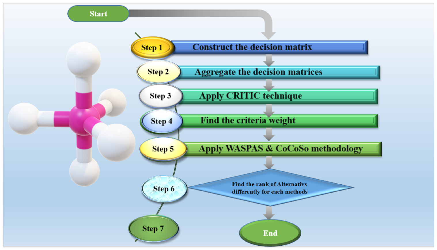
4.4. Pseudo Code Depicting the Empirical Study Application

Set up the structure with n numbers of criteria and m numbers of alternatives. K numbers of decision-makers give their overview on their knowledge in linguistic terms on the decision matrix of m × n order. Then linguistic terms are transformed into G D H H χ F N . MCDM techniques are applied to find the weight of the criteria and rank the alternatives. The K decision matrix of m × n order is used as input data.
INPUT:K numbers of decision matrix of m × n order
OUTPUT: Ranking the alternatives
COMPUTE: Weight of the criteria
INITIALIZE: G D H H χ F N
OPERATION: CRITIC, WASPAS and CoCoSo
1  MERGE merge the K numbers of DMs inputs in decision matrix
2  THEN normalize the comparison matrix
3  FOR CRITIC
4        FIND comparison matrix used to evaluate linear correlation coefficients between
.              criteria to criteria
5        THEN compute the measure of conflict
6        FIND determine the weight of the criteria
7  END FOR
8  BEGIN WASPAS
9       COMPUTE calculation of the ranking of the alternatives using weighted
.                              normalization by using WSM and WPM from decision matrix
10  END WASPAS
11  BEGIN CoCoSo
12       COMPUTE calculation of the ranking of the alternatives on the basis of K r value
.                                  find the K r a , K r b and K r c using WSM and WPM from decision
.                                  matrix
13  END CoCoSo

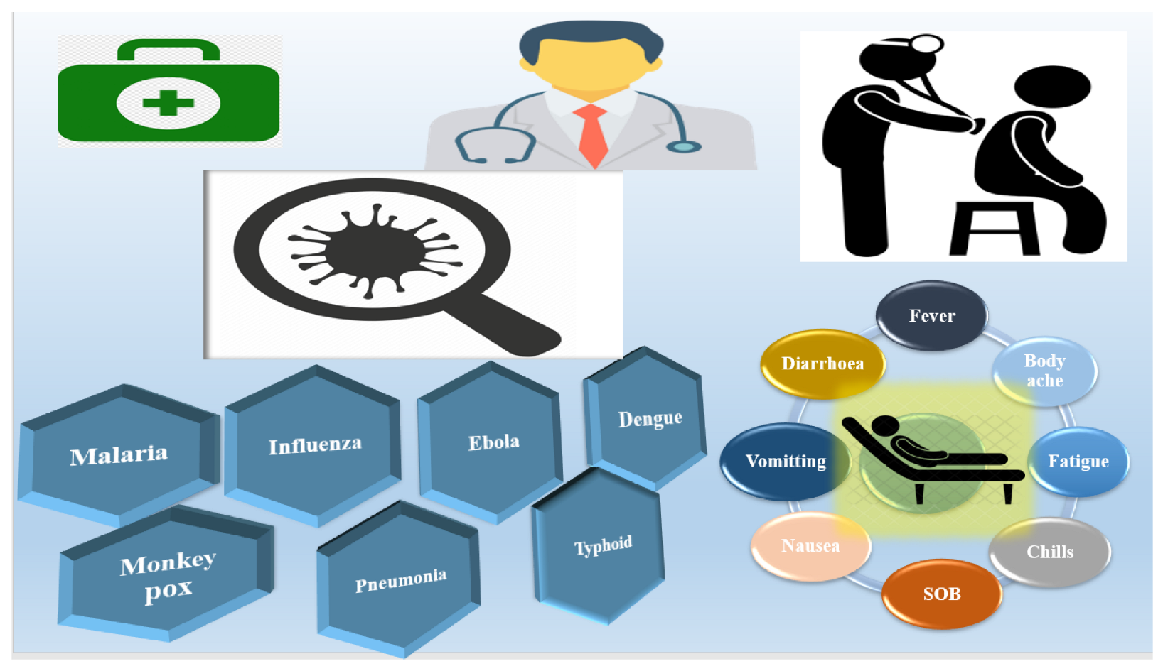
5. Brief Discussion of Alternative Diseases

In this section, we describe the details explanation of alternatives associated with the present model based on diseases recognition.

5.1. Malaria

Malaria [31,35,40] is often spread by mosquito bites from an infected female Anopheles mosquito. An infected person’s red blood cells contain the malaria parasite, which can also be spread through blood transfusions, organ transplants, and the shared use of needles or syringes tainted with blood. Additionally, before or during delivery, a mother’s unborn child may contract malaria from her. Malaria symptoms include fever and a flu-like disease with shivering chills, headache, muscular aches, and fatigue. Additionally, possible side effects include nausea, vomiting, and diarrhea. Due to the loss of red blood cells, malaria can result in anemia and jaundice (yellow skin and eyes).

5.2. Influenza

The influenza viruses [36,44,45,46] A, B, C, and D are the four different varieties of the virus. Influenza A virus (IAV), common in many animals, including humans and pigs, is primarily acquired through aquatic birds. The primary way influenza viruses spread among people is through respiratory droplets created when someone coughs or sneezes. Fever, sore muscles, sweats and chills, headache, shortness of breath, a persistent cough made of dryness, weakness and exhaustion, runny or congested nose, throat pain, a headache, vomiting, and diarrhea are common, but more commonly in children than in adults.

5.3. Typhoid

A bacterial infection [28,41,43] called typhoid fever can spread throughout the body and harm numerous organs. It can lead to significant problems and even be fatal without early treatment. Typically, contaminated food or water is how it is disseminated. The symptoms are high temperature, headache, nausea, weakness, and loose feces.

5.4. Dengue

Dengue [23,33,37,39] is a viral disease transmitted to humans through the bites of infected Aedes mosquitoes, primarily Aedes aegypti. The symptoms of dengue can range from mild to severe and usually appear between 3 and 14 days after infection. Dengue fever is typically characterized by a sudden onset of a high fever lasting several days. Additionally, people with dengue fever may experience severe headaches, particularly behind the eyes. High temperature, headache, muscle aches, nausea, and vomiting are the main symptoms of this disease. There is no specific treatment for dengue fever, and supportive care is often the only option.

5.5. Monkey Pox

Anyone can contract monkeypox [29,30] through close, direct, frequently skin-to-skin contact. A rash on the hands, feet, chest, face, or mouth appears in monkeypox patients. The flu, chills, enlarged lymph nodes, exhaustion, back pain, muscle aches, headache, and respiration issues (e.g., sore throat, nasal congestion, or cough) have also been observed in patients.

5.6. Ebola

The Ebola virus [38,42] causes severe, and frequently fatal, sicknesses known as Ebola virus disease (EVD), also referred to as Ebola hemorrhagic fever. It was first discovered during an outbreak in Sudan and the Democratic Republic of the Congo in 1976. Several attacks have since occurred in Africa, with the biggest being in West Africa between 2014 and 2016. People who come into contact with an infected bat or non-human primate or a sick or deceased Ebola virus-infected person directly may obtain EVD. Fever, aches and pains, such as a bad headache and painful muscles and joints, weakness, exhaustion, stiff neck, appetite loss, abdominal pain, diarrhea, vomiting, unexplained bleeding, bruising, or hemorrhaging are gastrointestinal symptoms. Red eyes, a rash, and hiccups are other symptoms that could occur (late-stage).

5.7. Pneumonia

A lung infection known as pneumonia [32,34] causes lung tissue swelling or inflammation. Viruses or bacterial infections are frequently to blame. Pneumonia symptoms may appear suddenly throughout 24 to 48 h or more gradually over several days. Chest pain, sweating, shivering, a cough, trouble breathing, a fast heartbeat, a high temperature, and an overall feeling of unwellness are symptoms.

6. Symptom of Disease and Model Setup

In this section, we describe the criteria for the proposed model. Figure 6 show how a doctor diagnoses a patient based on their symptoms and how to computationally identify and rank of disease.
In this section, let us choose the alternative disease mentioned by D 1 , D 2 , D 3 , D 4 , D 5 , D 6 , D 7 among the above-described disease of Section 5. We do not want to reveal the identity of the disease the patient has because we only want to demonstrate how our methodology can be used to diagnose patients.
Remark 5.
There are usually many factors to take to think about when diagnosing a disease, and the level of certainty for each factor can vary. Hexagonal fuzzy numbers ( H χ F N ) allow for a more flexible representation of uncertainty compared to traditional fuzzy numbers. This idea is expanded upon by the use of dual hesitant hexagonal fuzzy numbers ( D H H χ F N ) , which provide the expression of both positive and negative degrees of hesitation for a disease. G D H H χ F N s are particularly useful because they can represent not only the degree of membership but also the degree of non-membership and the degree of hesitancy in a more generalized way to capture any symptoms of the disease. This can help people make more informed judgments by accounting for a wider range of factors. Aside from this, it has been demonstrated that G D H H χ F N s are computationally efficient in several types of operations, including addition, subtraction, multiplication, and division. This can be beneficial for disease recognition where there are often many calculations involved in the diagnosis process. Overall, using G D H H χ F N s can offer a more adaptable, precise, and effective method of identifying diseases, improving diagnosis and therapeutic outcomes.

7. Data Collection

In this section, how the data are collected for the numerical study is shown briefly. There are three decision-makers from whom we obtained the data about patients. The experts are given below:
  • DM1: MD-Internal Medicine, MBBS General Physician
  • DM2: MBBS, MD-Medicine, MD-USC, California, General Physician
  • DM3: MBBS, MD-Pediatrics, MRCP (UK), Diploma in Child Health (DCH), Pediatrician
In this study, eight factors have been considered to recognize the disease in a patient. This concept has been taken from the author of [97]. Let there be the n numbers of diseases and the m numbers of symptoms associated with these diseases. If a patient V has almost all these symptoms, recognizing the disease becomes cumbersome. Hence, to capture this hesitancy or uncertainty, G D H H χ F N has been used with MCDM tools WASPAS and CoCoSo to identify the specific medical problem and understand the exact diagnosis required for that patient. The eight symptoms considered are fever, body ache, fatigue, chills, shortness of breath (SOB), nausea, vomiting, and diarrhea. The symptoms have been weighted by another MCDM technique CRITIC. Seven alternatives have been taken for the study. The symptoms have been assigned linguistic terms with regard to obtaining the ranking, and another MCDM technique CoCoSo is used to verify the robustness of our result. G D H H χ F N with WASPAS and CoCoSo model is applied to rank the treatment alternatives. Some steps of our methodology are shown in a later section.
Table 6 shows the linguistic term and corresponding G D H H c h i F N with their defuzzified values. In Table 7, we display the decision-makers (DMs) rating in linguistic terms.

8. Numerical Description

The numerical simulation is performed in this section. We give the details explanation how the data are fitted to the proposed model and how the proposed method is applied for finding the numerical solution.
First, we gather information from three decision-makers in distinct ways, which are shown in Table 7. The linguistic variables are represented by G D H H χ F N second type of Table 6. Then we aggregate the three decision-makers’ opinions into a single decision matrix using the Equation (41). Then using FCRITIC method mentioned in Section 4.1 evaluates the symptoms or criteria weights, which are shown in Table 8.
Using decision matrix in Table 7 and criteria weight (from Table 8), calculate the alternative ranking by FWASPAS methodology, which mentioned in Section 4.2 are shown in Table 9.
Using the FWASPAS data (from Table 9) and the FCoCoSo technique mentioned in Section 4.3, calculate alternatives ranking are shown in Table 10.
Remark 6.
When aggregated the three decision-makers, we obtain same rank of disease alternatives in both WASPAS and CoCoSo methods, which is demonstrated in Table 9 and Table 10 and Figure 7. D 1 , D 2 , D 3 , D 4 , D 5 , D 6 , D 7 are at the rank 7, 1, 5, 6, 4, 3, 2 in both systems, respectively.

Computational Complexity

This section discusses the computational complexity of this proposed fuzzy MCDM model. The idea of this numerical analysis is mentioned in several studies [98]. The total number of numerical calculations conducted to obtain the solution is described by time complexity and denoted by T c . Here, we assume n numbers of criteria and m numbers of alternatives are performed in the evaluation process. Total K numbers of DMs give their decision in G D H H χ F N . Then, the following steps are considered to reach the solution.
  • For the FCRITIC method, the K decision matrices have m × n entries. Then, the aggregated decision matrix has m × n operations. To de-fuzzifies the decision matrix, another m × n operation are conducted. Normalizing the decision matrix m × n + 2 n calculation are performed. Calculate the standard division by n number of operations. We performed n 2 operation to find the correlation coefficients. To measure the conflict created by the criteria, n 2 operations are conducted. Finally, obtain the criteria weight by conducted 2 n + 1 operations. Total operations performed for the FCRITIC method are m n + m n + m n + 2 n + n + n 2 + n 2 + 2 n + 1 = 3 m n + 2 n 2 + 5 n + 1 .
  • For the FWASPAS technique, from the FCRITIC method, we already obtain aggregated decision matrix. Then, normalize the aggregated decision matrix by conducting m × n + n operations. Another m × n calculations was performed to the weighted sum decision matrix. To de-fuzzified the weighted sum decision matrix m × n operations operated and weighted sum value calculated by m operations. Similarly, finding to weighted product decision matrix, de-fuzzification, and weighted product value m × n , m × n , and m operations performed, respectively. Finally, to rank the alternatives 2 m operations are conducted. Then, the total calculations conducted for the FWASPAS method are m n + n + m n + m n + m + m n + m n + m + 2 m = 5 m n + 4 m + n .
  • For the FCoCoSo method, form the FCRITIC and the FWASPAS methods, we already obtain weighted sum value and weighted product value. Then, to calculate K ζ a , K ζ b and K ζ c values 3 m operations conducted. Finally, to rank the alternatives on the basis of 2 m operations. Total calculation conducted for the FCoCoSo method are 3 m + 2 m = 5 m .
In this study, time complexity ( T c ) is calculated by criteria n = 8 , alternative m = 7 , and decision-maker K = 3 as follows:
  • For FCRITIC, number of calculation are 3 × 7 × 8 + 2 × 8 2 + 5 × 8 + 1 = 337 .
  • For FWASPAS, number of operations are 5 × 7 × 8 + 4 × 7 + 8 = 316 .
  • For FCoCoSo, number of operations are 5 × 7 = 35 .
The time complexity of this study is 337 + 316 + 35 = 688 .

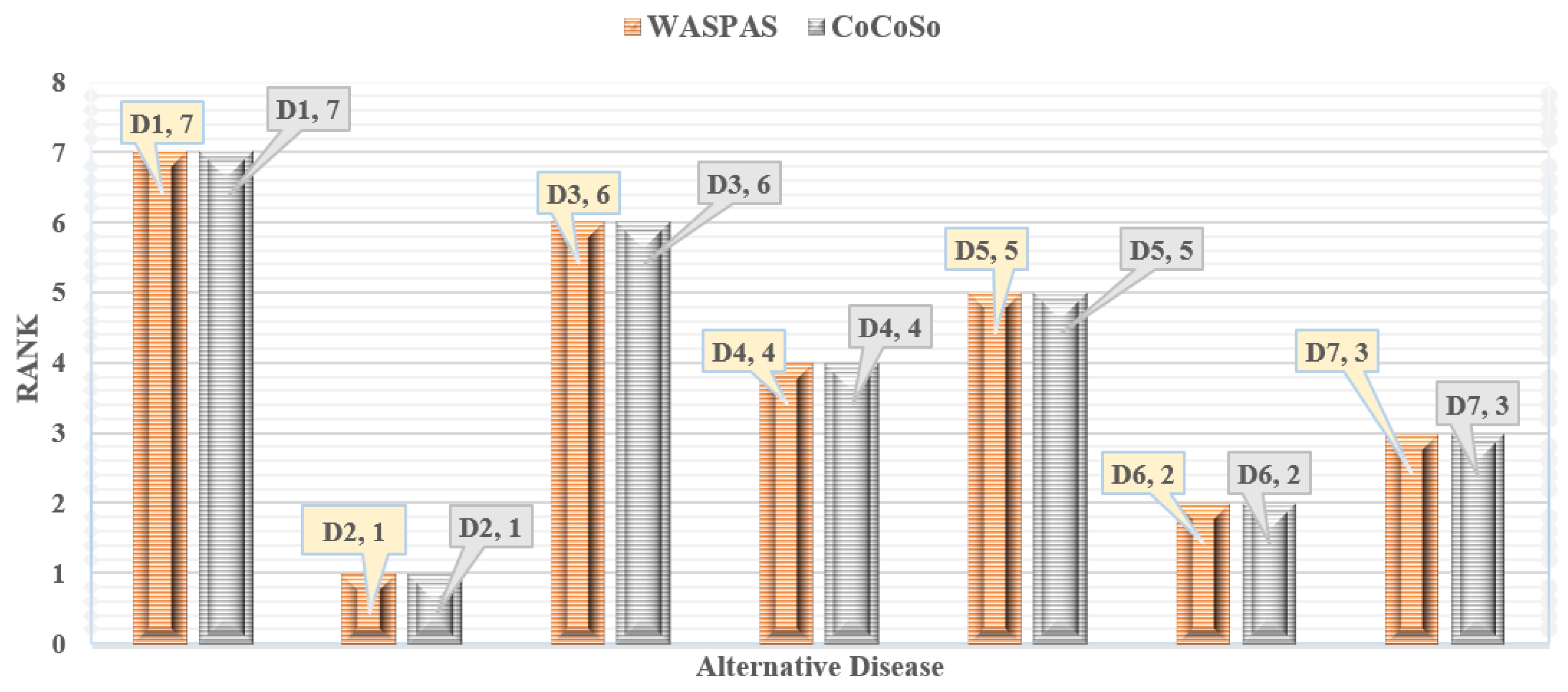
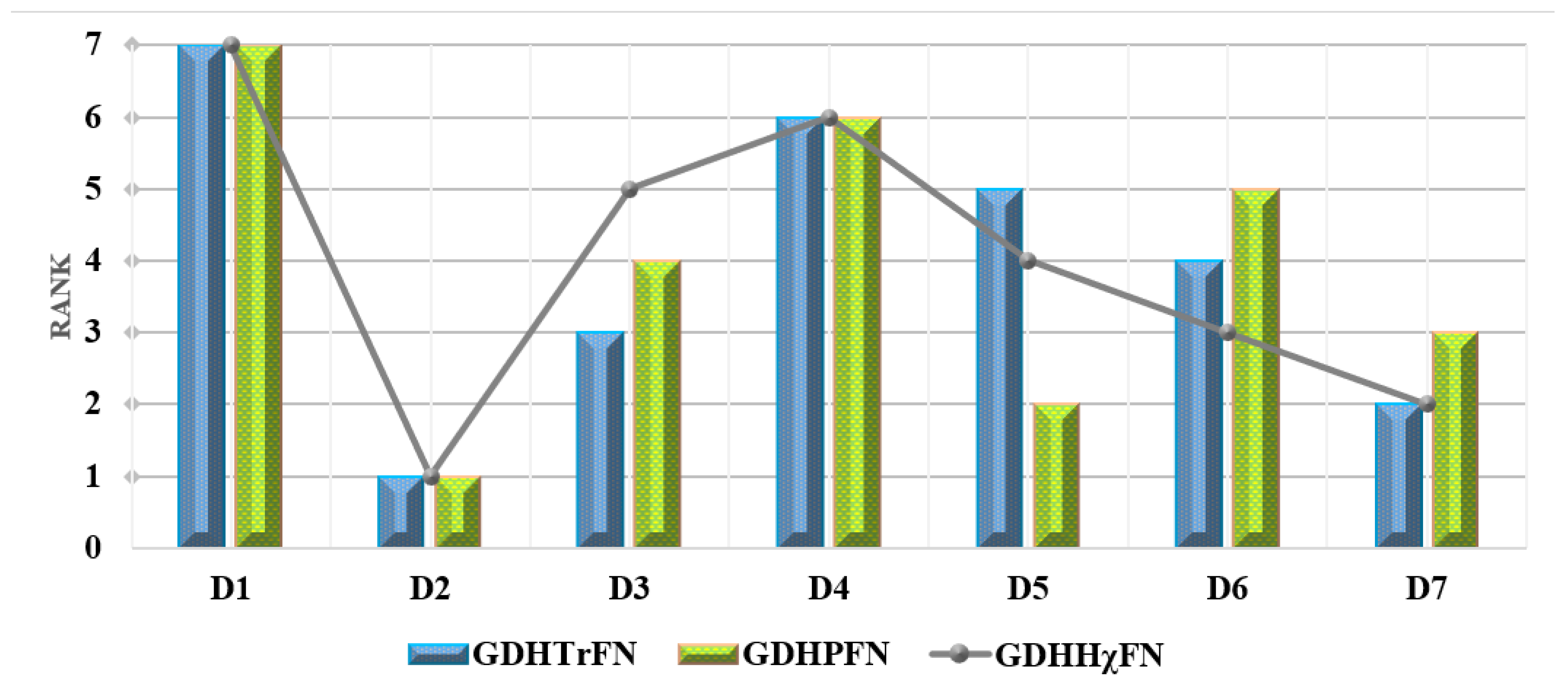
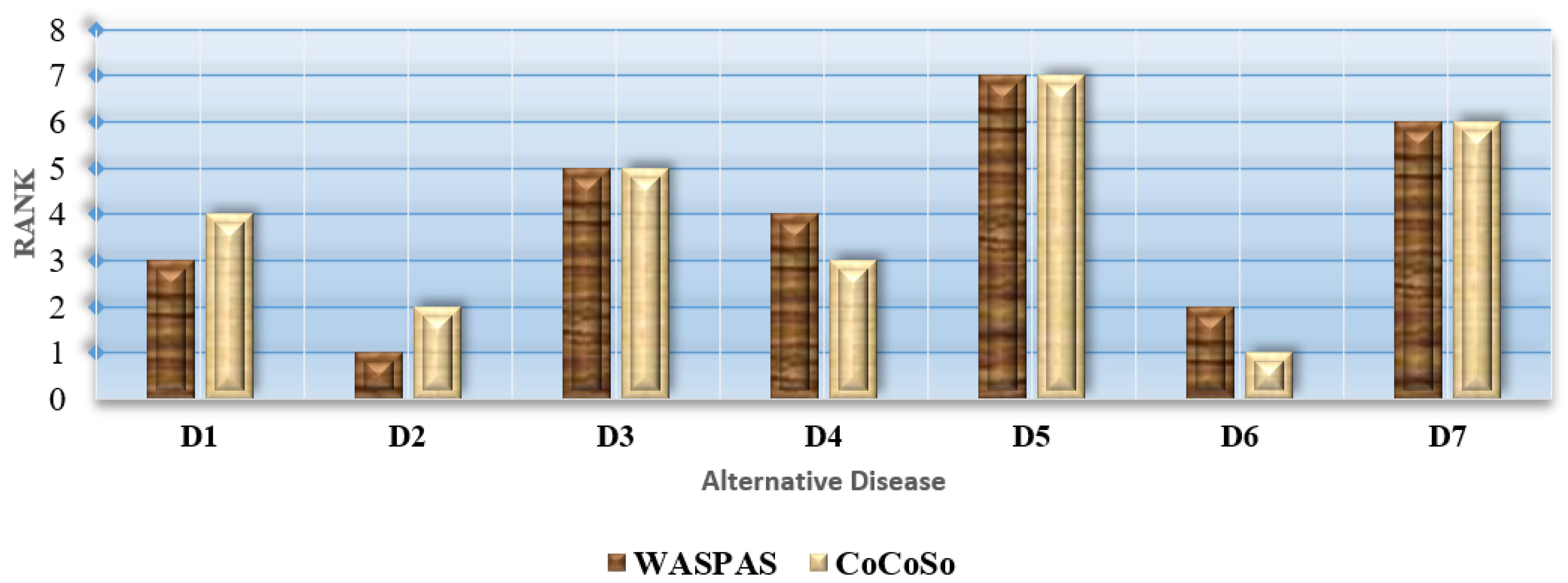
9. Sensitivity Analysis and Comparative Analysis

We are interested to find some crucial results for decision-making problems in different cases. We must conduct a sensitivity analysis and comparative analysis to accomplish that. The accuracy of the final result may, therefore, be affected by initial criteria, parameters, data and measures, so doing a sensitivity analysis will aid in identifying the important factors. Additionally, the different fuzzy number gives the solutions flexibility and robustness using comparative analysis.

9.1. Sensitivity Analysis

In this section, we have considered three more patients V 1 , V 2 , and V 3 . While interacting with them regarding the ailments they are suffering, we came across varied symptoms.
Case 1: The patient V 1 informed that fever and chills, these two symptoms were quite less on an average. So, the rating of fever and chills are removed. Considering this case, the ranking indicates that the patient is suffering from D 2 .
Remark 7.
The ranking of these alternative diseases is also same when we eliminate the criteria fever and chills, which is shown in Table 11 and Figure 8. The diseases D 1 , D 2 , D 3 , D 4 , D 5 , D 6 , D 7 are ranked as rank 6, 1, 5, 7, 4, 2, 3 in both WASPAS and CoCoSo, respectively.
Case 2: The patient V 2 informed that body ache and fatigue, these two symptoms were negligible or very less on an average. The ranking so obtained considering this case indicates that the patient is also suffering from D 2 .
Remark 8.
In this case the Table 12 and Figure 9 show, there are no change in rank of the alternatives, when the criteria body ache and fatigue are removed. The alternatives diseases D 1 , D 2 , D 3 , D 4 , D 5 , D 6 , and D 7 have the same rank as 7, 1, 6, 4, 5, 2, 3, respectively, in both system WASPAS and CoCoSo.
Case 3: The patient V 3 informed that SOB and nausea, these two symptoms have no issue. The ranking so obtained reveals that the patient is suffering from D 2 or D 6 .
Remark 9.
Here, the Table 13 and the Figure 10 show that the ranking of alternative diseases are completely altered for removing the criteria SOB and Nausea. The rank of the alternatives D 1 , D 2 , D 3 , D 4 , D 5 , D 6 , and D 7 are 3, 1, 5, 4, 7, 2, and 6, respectively, in WASPAS, and 4, 2, 5, 3, 7, 1, and 6, respectively, in CoCoSo.
Considering these three cases of the three individual patients, transforming the linguistic rating to G D H H χ FN, the ranking obtained are represented in Table 11, Table 12 and Table 13 and Figure 8, Figure 9 and Figure 10, respectively.

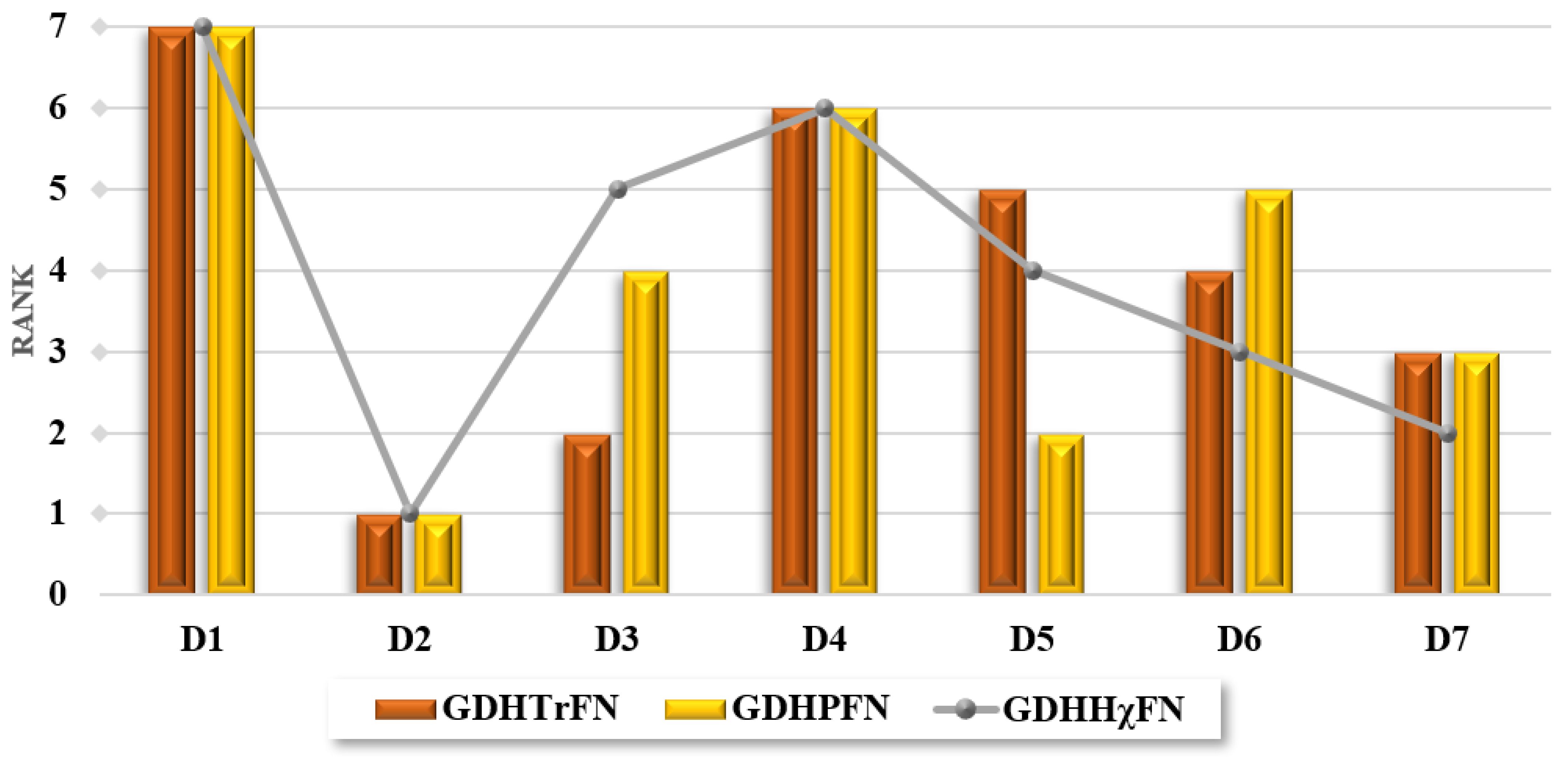
9.2. Comparative Analysis

We would need to examine using three different fuzzy numbers in order to check the consistency and reliability of our procedures, as well as the accuracy and specificity of our results. In addition to G D H H χ F N , we also used two other fuzzy numbers which are generalized dual hesitant trapizoidal fuzzy number ( G D H T r F N ) and generalized dual hesitant pentagonal fuzzy number ( G D H P F N ). Table 14 shows the rank of alternative disease by G D H T r F N , G D H P F N , G D H H χ F N , respectively, in WASPAS and CoCoSo methods.
Remark 10.
Table 14 and Figure 11 and Figure 12 depict that the disease D 2 is at rank 1 for each three fuzzy numbers in both methods WASPAS and CoCoSo, and the rank of remaining diseases are slightly changed. For G D H T r F WASPAS and CoCoSo, D 1 , D 4 , D 5 , and D 6 have same rank which are 7, 6, 5, and 4, respectively, and D 3 have rank 2 and 3 and D 7 have rank 3 and 2. In the same way, for G D H P F N and G D H H χ F N , all diseases have the same rank for both methods WASPAS and CoCoSo, respectively, which is displayed in Table 14.
Finally, we observe that in each fuzzy environment using the provided MCDM methodologies, the disease D 2 is always at rank 1. Hence, we may conclude with certainty that the patient has the disease D 2 .

10. Practical Implications

The whole study is based on the symptomatic dataset and statistical analysis. The proposed methodology is to find the most changes among the related diseases. Therefore, this method can be used entirely for clustering the presence of associated diseases with typical symptoms. Before the lab test or consulting with a medical supervisor, anyone can easily find the related illnesses they suffer. As it is common to be reliant on technology, whether it be a laptop, smartwatch, or mobile phone, it may be easy to store data for analysis purposes. This work only shows how the decision may be taken after the mathematical and numerical analyses. Suppose any software is made to take data about symptoms from an infected person, then uses the proposed algorithm to conclude that initial disease identification and move forward to analysis and lab tests.

11. Conclusions and Future Research Extension

In conclusion, this research study has focused on exploring the applicability of the multi-criteria decision-making (MCDM) technique using Generalized Dual Hesitant Hexagonal Fuzzy Number ( G D H H χ F N ) for the diagnosis of the patient. The study has demonstrated the effectiveness of the proposed strategy in dealing with ambiguity and the uncertainty that is prevalent in the medical diagnosis process.

11.1. Summary of Study and Contributions

The study of disease recognition by the generalized dual hesitant hexagonal fuzzy MCDM technique is an approach to evaluate and recognize diseases based on multiple criteria. The proposed method uses a combination of dual hesitant fuzzy set theory and hexagonal fuzzy numbers to model the uncertain and imprecise information associated with disease recognition. This study provides a valuable contribution to the field of medical diagnosis by introducing a new approach to decision-making that is more accurate, comprehensive, and efficient. The contributions of our study are as follows:
(a)
In order to compare each G D H H χ F N , we have first proposed a new defuzzification technique for a G D H H χ F N and modified the arithmetic operation of G D H H χ F N first type and second type.
(b)
Then, we develop an aggregation formula to combine more than one decision matrix.
(c)
Here, we have used the FCRITIC approach to determine the weight of the criteria (symptom).
(d)
We have applied the FWASPAS and FCoCoSo methods simultaneously to determine the rank of the alternatives (Disease).
(e)
Finally, we conducted a comparative analysis using two alternative fuzzy numbers, G D H P F N and G D H T r F N .

11.2. The Crucial Findings

The G D H H χ F MCDM approach can successfully handle the uncertainty and ambiguity involved with medical diagnosis, which is an important finding of these studies. Specifically, the technique enables the representation of decision-making criteria and alternatives using dual hesitant fuzzy sets, which are a particular kind of fuzzy set that allows decision-makers to express their degree of hesitation or uncertainty about the membership and non-membership of an element in a set. The hexagonal structure of the dual hesitant fuzzy sets used in the G D H H χ F MCDM technique provides more flexibility in representing the degree of hesitancy. Overall, the use of the G D H H χ F MCDM technique in disease recognition has shown promising results and can potentially be used as a tool to aid medical professionals in making more informed decisions in the diagnosis of diseases.

11.3. The Restriction and Directions for Future Research

The proposed approach has been validated through a case study on the diagnosis of patients, and the results have shown that it can produce accurate and reliable outcomes compared to other existing methods. Therefore, the use of G D H H χ F N based MCDM technique can be considered a promising approach for medical diagnosis applications. We have used seven alternative diseases and eight criteria (symptoms) to diagnose a patient.
However, further research is necessary to investigate the generalization of this approach to other diseases and to explore the potential of integrating additional data sources, such as patient history, laboratory test results, and medical imaging, by another generalized fuzzy environment with a new de-fuzzification method. More criteria and alternatives can be taken to identify a patient’s disease. Overall, this research paper has contributed to the growing body of literature on the application of MCDM techniques in medical diagnosis, and it has demonstrated the potential of G D H H χ F N based MCDM for accurate and reliable disease diagnosis.

Author Contributions

Conceptualization, A.F.M., S.M., K.H.G., and B.C.G.; Methodology, A.F.M., S.M., K.H.G., B.C.G., and S.P.M.; Formal analysis, A.F.M.; Resources, A.F.M., S.M., and B.C.G.; Software, A.F.M., S.M., and K.H.G.; Investigation, A.F.M., K.H.G., B.C.G., and S.P.M.; Validation, A.F.M.; Writing—original draft preparation, A.F.M., S.M., and S.P.M.; Writing—review and editing, A.F.M.; Supervision, B.C.G.; funding acquisition, A.F.M. All authors equally contribute in every section. All authors have read and agreed to the published version of the manuscript.

Funding

This study is supported via funding from Prince Sattam Bin Abdulaziz University project number PSAU/2023/R/1444.

Data Availability Statement

The used data are already in this manuscript. The data sources are also clearly mentioned.

Conflicts of Interest

The authors declare that there are no conflicts of interest in this study.

References

  1. Lee, B.; Yun, Y.S. The generalized trapezoidal fuzzy sets. J. Chungcheong Math. Soc. 2011, 24, 253–266. [Google Scholar]
  2. Deli, I. A TOPSIS method by using generalized trapezoidal hesitant fuzzy numbers and application to a robot selection problem. J. Intell. Fuzzy Syst. 2020, 38, 779–793. [Google Scholar] [CrossRef]
  3. Chen, S.J.; Chen, S.M. Fuzzy risk analysis based on similarity measures of generalized fuzzy numbers. IEEE Trans. Fuzzy Syst. 2003, 11, 45–56. [Google Scholar] [CrossRef]
  4. Xu, P.; Su, X.; Wu, J.; Sun, X.; Zhang, Y.; Deng, Y. A note on ranking generalized fuzzy numbers. Expert Syst. Appl. 2012, 39, 6454–6457. [Google Scholar] [CrossRef]
  5. Li, G.; Kou, G.; Lin, C.; Xu, L.; Liao, Y. Multi-attribute decision making with generalized fuzzy numbers. J. Oper. Res. Soc. 2015, 66, 1793–1803. [Google Scholar] [CrossRef]
  6. Chen, T.Y. Multiple criteria group decision-making with generalized interval-valued fuzzy numbers based on signed distances and incomplete weights. Appl. Math. Model. 2012, 36, 3029–3052. [Google Scholar] [CrossRef]
  7. Pedrycz, W. On generalized fuzzy relational equations and their applications. J. Math. Anal. Appl. 1985, 107, 520–536. [Google Scholar] [CrossRef] [Green Version]
  8. Keikha, A. Generalized hesitant fuzzy numbers and their application in solving MADM problems based on TOPSIS method. Soft Comput. 2022, 26, 4673–4683. [Google Scholar] [CrossRef]
  9. Wan, S.; Dong, J.; Chen, S.M. Fuzzy best-worst method based on generalized interval-valued trapezoidal fuzzy numbers for multi-criteria decision-making. Inf. Sci. 2021, 573, 493–518. [Google Scholar] [CrossRef]
  10. Song, Y.; Hu, J. Vector similarity measures of hesitant fuzzy linguistic term sets and their applications. PLoS ONE 2017, 12, E0189579. [Google Scholar] [CrossRef] [Green Version]
  11. Liao, H.; Xu, Z.; Zeng, X.J.; Merigó, J.M. Qualitative decision making with correlation coefficients of hesitant fuzzy linguistic term sets. Knowl.-Based Syst. 2015, 76, 127–138. [Google Scholar] [CrossRef]
  12. Mardani, A.; Saraji, M.K.; Mishra, A.R.; Rani, P. A novel extended approach under hesitant fuzzy sets to design a framework for assessing the key challenges of digital health interventions adoption during the COVID-19 outbreak. Appl. Soft Comput. 2020, 96, 106613. [Google Scholar] [CrossRef]
  13. Ghorui, N.; Ghosh, A.; Mondal, S.P.; Bajuri, M.Y.; Ahmadian, A.; Salahshour, S.; Ferrara, M. Identification of dominant risk factor involved in spread of COVID-19 using hesitant fuzzy MCDM methodology. Results Phys. 2021, 21, 103811. [Google Scholar] [CrossRef]
  14. Ali, W.; Shaheen, T.; Haq, I.U.; Toor, H.G.; Akram, F.; Jafari, S.; Uddin, M.Z.; Hassan, M.M. Multiple-Attribute Decision Making Based on Intuitionistic Hesitant Fuzzy Connection Set Environment. Symmetry 2023, 15, 778. [Google Scholar] [CrossRef]
  15. Lu, Y.; Xu, Y.; Huang, J.; Wei, J.; Herrera-Viedma, E. Social network clustering and consensus-based distrust behaviors management for large-scale group decision-making with incomplete hesitant fuzzy preference relations. Appl. Soft Comput. 2022, 117, 108373. [Google Scholar] [CrossRef]
  16. Aikhuele, D.O.; Odofin, S. A generalized triangular intuitionistic fuzzy geometric averaging operator for decision-making in engineering and management. Information 2017, 8, 78. [Google Scholar] [CrossRef] [Green Version]
  17. Rajendran, C.; Ananthanarayanan, M. Fuzzy criticalpath method with hexagonal and generalised hexagonal fuzzy numbers using ranking method. Int. J. Appl. Eng. Res. 2018, 13, 11877–11882. [Google Scholar]
  18. Ritmak, N.; Rattanawong, W.; Vongmanee, V. The dynamic evaluation model of health sustainability under MCDM benchmarking health indicator standards. Int. J. Environ. Res. Public Health 2022, 20, 259. [Google Scholar] [CrossRef]
  19. Mumtaz, A. Prioritizing and overcoming barriers to e-health use among elderly people: Implementation of the analytical hierarchical process (AHP). J. Healthc. Eng. Hindawi 2022, 2022, 7852806. [Google Scholar] [CrossRef] [PubMed]
  20. Yas, Q.M.; Adday, B.N.; Abed, A.S. Evaluation multi diabetes mellitus symptoms by integrated fuzzy-based MCDM approach. Turk. J. Comput. Math. Educ. 2021, 12, 4069–4082. [Google Scholar]
  21. Yildirim, F.S.; Sayan, M.; Sanlidag, T.; Uzun, B.; Ozsahin, D.U.; Ozsahin, I. Comparative evaluation of the treatment of COVID-19 with multi-criteria decision-making techniques. J. Healthc. Eng. Hindawi 2021, 2021, 8864522. [Google Scholar] [CrossRef]
  22. Nguyen, P.H.; Tsai, J.F.; Dang, T.T.; Lin, M.H.; Pham, H.A.; Nguyen, K.A. A hybrid spherical fuzzy MCDM approach to prioritize governmental intervention strategies against the COVID-19 pandemic: A case study from Vietnam. Mathematics 2021, 9, 2626. [Google Scholar] [CrossRef]
  23. Addy, M.; Chaudhuri, A.K.; Das, A. Role of data mining techniques and MCDM model in detection and severity monitoring to serve as precautionary methodologies against ‘Dengue’. In Proceedings of the International Conference on Computer Science, Engineering and Applications (ICCSEA), Gunupur, India, 13–14 March 2020; pp. 1–6. [Google Scholar] [CrossRef]
  24. Mohammed, M.A.; Abdulkareem, K.H.; Al-Waisy, A.S.; Mostafa, S.A.; Al-Fahdawi, S.; Dinar, A.M.; Alhakami, W.; Baz, A.; Al-Mhiqani, M.N.; Alhakami, H.; et al. Benchmarking methodology for selection of optimal COVID-19 diagnostic model based on entropy and TOPSIS methods. IEEE Access 2020, 8, 99115–99131. [Google Scholar] [CrossRef]
  25. Abdel-Basset, M.; Gamal, A.; Manogaran, G.; Son, L.H.; Long, H.V. A novel group decision making model based on neutrosophic sets for heart disease diagnosis. Multimed. Tools Appl. 2020, 79, 9977–10002. [Google Scholar] [CrossRef]
  26. Sharawat, K.; Dubey, S.K. Diet recommendation for diabetic patients using MCDM approach. Adv. Intell. Syst. Comput. 2018, 624, 239–246. [Google Scholar] [CrossRef]
  27. Basanta, H.; Huang, Y.P.; Lee, T.T. Intuitive IoT-based H2U healthcare system for elderly people. In Proceedings of the 13th International Conference on Networking, Sensing, and Control (ICNSC), Mexico City, Mexico, 28–30 April 2016; pp. 1–6. [Google Scholar] [CrossRef]
  28. Uzoka, F.M.; Nwokoro, C.; Obot, O.; Ekpenyong, M.; Udo, A.I.A.; Akinnuwesi, B. Analytic hierarchy process model for the diagnosis of typhoid fever. In Proceedings of the Future Technologies Conference (FTC), Vancouver, Canada, 21–23 October 2022; pp. 341–358. [Google Scholar] [CrossRef]
  29. Fantini, J.; Chahinian, H.; Yahi, N. A vaccine strategy based on the identification of an annular ganglioside binding motif in Monkeypox virus protein E8L. Viruses 2022, 14, 2531. [Google Scholar] [CrossRef]
  30. Kaler, J.; Hussain, A.; Flores, G.; Kheiri, S.; Desrosiers, D. Monkeypox: A comprehensive review of transmission, pathogenesis, and manifestation. Cureus 2022, 14, e26531. [Google Scholar] [CrossRef]
  31. Nakasi, R.; Mwebaze, E.; Zawedde, A. Mobile-aware deep learning algorithms for malaria parasites and white blood cells localization in thick blood smears. Algorithms 2021, 14, 17. [Google Scholar] [CrossRef]
  32. Abodayeh, K.; Raza, A.; Rafiq, M.; Arif, M.S.; Naveed, M.; Zeb, Z.; Abbas, S.Z.; Shahzadi, K.; Sarwar, S.; Naveed, Q.; et al. Analysis of pneumonia model via efficient computing techniques; Computers, Materials & Continua. Mater. Contin. 2021, 70, 6073–6088. [Google Scholar] [CrossRef]
  33. Bhuju, G.; Phaijoo, G.R.; Gurung, D.B. Fuzzy approach analyzing SEIR-SEI dengue dynamics. Biomed Res. Int. 2020, 2020, 1508613. [Google Scholar] [CrossRef]
  34. Nathan, A.M.; Teh, C.S.J.; Jabar, K.A.; Teoh, B.T.; Tangaperumal, A.; Westerhout, C.; Zaki, R.; Eg, K.P.; Thavagnanam, S.; Bruyne, J.A.D. Bacterial pneumonia and its associated factors in children from a developing country: A prospective cohort study. PLoS ONE 2020, 15, e0228056. [Google Scholar] [CrossRef] [PubMed]
  35. Modibbo, U.M.; Heman, E.D.; Hafisu, R. Multi-criteria decision analysis for malaria control strategies using analytic hierarchy process: A case of Yola North local government area, Adamawa state Nigeria. Amity J. Comput. Sci. (Ajcs) 2019, 3, 43–50. [Google Scholar]
  36. Samanlioglu, F. Evaluation of influenza intervention strategies in Turkey with fuzzy AHP-VIKOR. J. Healthc. Eng. 2019, 2019, 9486070. [Google Scholar] [CrossRef] [Green Version]
  37. Majid, N.A.; Nazi, N.M.; Mohamed, A.F. Distribution and spatial pattern analysis on dengue cases in Seremban district, Negeri Sembilan, Malaysia. Sustainability 2019, 11, 3572. [Google Scholar] [CrossRef] [Green Version]
  38. Martin, N.; Ritha, W.; Vinoline, I.A.; Selvi, P. Analysis of the risk of ebola disease: Fuzzy VIKOR method based on the possibility theory. Int. J. Manag. Appl. Sci. 2019, 5, 37–40. [Google Scholar]
  39. Gbadamosi, B.; Ojo, M.M.; Oke, S.I.; Matadi, M.B. Qualitative analysis of a dengue fever model. Math. Comput. Appl. 2018, 23, 33. [Google Scholar] [CrossRef] [Green Version]
  40. Kim, J.Y.; Eun, S.J.; Park, D.K. Malaria vulnerability map mobile system development using GIS-based decision-making technique. Locat.-Based Mob. Mark. Innov. 2018, 2018, 8436210. [Google Scholar] [CrossRef] [Green Version]
  41. Tilahun, G.T.; Makinde, O.D.; Malonza, D. Modelling and optimal control of typhoid fever disease with cost-effective strategies. Comput. Math. Methods Med. 2017, 2017, 2324518. [Google Scholar] [CrossRef] [Green Version]
  42. Kourtis, A.P.; Appelgren, K.; Chevalier, M.S.; McElroy, A. Ebola virus disease focus on children. Pediatr. Infect. Dis. J. 2015, 34, 893–897. [Google Scholar] [CrossRef] [Green Version]
  43. Dewan, A.M.; Corner, R.; Hashizume, M.; Ongee, E.T. Typhoid fever and its association with environmental factors in the Dhaka metropolitan area of Bangladesh: A spatial and time-series approach. PLoS Neglected Trop. Dis. 2013, 7, e1998. [Google Scholar] [CrossRef] [Green Version]
  44. Araz, O.M. Integrating complex system dynamics of pandemic influenza with a multi-criteria decision making model for evaluating public health strategies. J. Syst. Sci. Syst. Eng. 2013, 22, 319–339. [Google Scholar] [CrossRef]
  45. Zhang, J.; Lu, J.; Zhang, G. Combining one class classification models for avian influenza outbreaks. In Proceedings of the Symposium on Computational Intelligence in Multicriteria Decision-Making (MDCM), Paris, France, 11–15 April 2011; pp. 1–7. [Google Scholar] [CrossRef]
  46. Attaluri, P.K.; Chen, Z.; Weerakoon, A.M.; Lu, G. Integrating decision tree and hidden markov model (HMM) for subtype prediction of human influenza a virus. In Cutting-Edge Research Topics on Multiple Criteria Decision Making; Springer: Berlin/Heidelberg, Germany, 2009; Volume 35, pp. 52–58. [Google Scholar] [CrossRef]
  47. Sindhu, M.S.; Rashid, T. Selection of alternative based on linear programming and the extended fuzzy TOPSIS under the framework of dual hesitant fuzzy sets. Soft Comput. 2023, 27, 1985–1996. [Google Scholar] [CrossRef]
  48. Ismael, S.F.; Alias, A.H.; Zaidan, A.A.; Zaidan, B.B.; Alsattar, H.A.; Qahtan, S.; Albahri, O.S.; Talal, M.; Alamoodi, A.H.; Mohammed, R.T. Toward sustainable transportation: A pavement strategy selection based on the extension of dual-hesitant fuzzy multicriteria decision-making methods. IEEE Trans. Fuzzy Syst. 2023, 31, 380–393. [Google Scholar] [CrossRef]
  49. Kang, D.; Anuja, A.; Narayanamoorthy, S.; Gangemi, M.; Ahmadian, A. A dual hesitant q-rung orthopair enhanced MARCOS methodology under uncertainty to determine a used PPE kit disposal. Environ. Sci. Pollut. Res. 2022, 29, 89625–89642. [Google Scholar] [CrossRef]
  50. Calache, L.D.D.R.; Camargo, V.C.B.; Osiro, L.; Carpinetti, L.C.R. A genetic algorithm based on dual hesitant fuzzy preference relations for consensus group decision making. Appl. Soft Comput. 2022, 121, 108778. [Google Scholar] [CrossRef]
  51. Ni, Y.; Zhao, H.; Xu, Z.; Wang, Z. Multiple attribute decision-making method based on projection model for dual hesitant fuzzy set. Fuzzy Optim. Decis. Mak. 2022, 21, 263–289. [Google Scholar] [CrossRef]
  52. Guirao, J.L.G.; Sindhu, M.S.; Rashid, T.; Kashif, A. Multiple criteria decision-making based on vector similarity measures under the framework of dual hesitant fuzzy sets. Discret. Dyn. Nat. Soc. 2020, 2020, 1425487. [Google Scholar] [CrossRef]
  53. Garg, H.; Kaur, G. Quantifying gesture information in brain hemorrhage patients using probabilistic dual hesitant fuzzy sets with unknown probability information. Comput. Ind. Eng. 2020, 140, 106211. [Google Scholar] [CrossRef]
  54. Ren, Z.; Xu, Z.; Wang, H. The strategy selection problem on artificial intelligence with an integrated VIKOR and AHP method under probabilistic dual hesitant fuzzy information. IEEE Access 2019, 7, 103979–103999. [Google Scholar] [CrossRef]
  55. Chen, H.; Xu, G.; Yang, P. Multi-attribute decision-making approach based on dual hesitant fuzzy information measures and their applications. Mathematics 2019, 7, 786. [Google Scholar] [CrossRef] [Green Version]
  56. Narayanamoorthy, S.; Ramya, L.; Baleanu, D.; Kureethara, J.V.; Annapoorani, V. Application of normal wiggly dual hesitant fuzzy sets to site selection for hydrogen underground storage. Int. J. Hydrogen Energy 2019, 44, 28874–28892. [Google Scholar] [CrossRef]
  57. Liu, P.; Cheng, S. Interval-valued probabilistic dual hesitant fuzzy sets for multi-criteria group decision-making. Int. J. Comput. Intell. Syst. 2019, 12, 1393–1411. [Google Scholar] [CrossRef] [Green Version]
  58. Hao, Z.; Xu, Z.; Zhao, H.; Su, Z. Probabilistic dual hesitant fuzzy set and its application in risk evaluation. Knowl.-Based Syst. 2017, 127, 16–28. [Google Scholar] [CrossRef]
  59. Deli, I.; Karaaslan, F. Generalized trapezoidal hesitant fuzzy numbers and their applications to multi criteria decision-making problems. Soft Comput. 2021, 25, 1017–1032. [Google Scholar] [CrossRef]
  60. Sultan, A.; Sałabun, W.; Faizi, S.; Ism, M. Hesitant fuzzy linear regression model for decision making. Symmetry 2021, 13, 1846. [Google Scholar] [CrossRef]
  61. Büyüközkan, G.; Güler, M. A combined hesitant fuzzy MCDM approach for supply chain analytics tool evaluation. Appl. Soft Comput. 2021, 112, 107812. [Google Scholar] [CrossRef]
  62. Farid, H.M.A.; Riaz, M. Some generalized q-rung orthopair fuzzy Einstein interactive geometric aggregation operators with improved operational laws. Int. J. Intell. Syst. 2021, 36, 7239–7273. [Google Scholar] [CrossRef]
  63. Zulqarnain, R.M.; Saeed, M.; Ali, B.; Abdal, S.; Saqlain, M.; Ahamad, M.I.; Zafar, Z. Generalized fuzzy TOPSIS to solve multi-criteria decision-making problems. J. New Theory 2020, 32, 40–50. [Google Scholar]
  64. Yue, Q.; Zhang, L. Two-sided matching for hesitant fuzzy numbers in smart intelligent technique transfer. Mech. Syst. Signal Process. 2020, 139, 106643–106653. [Google Scholar] [CrossRef]
  65. Garg, H.; Keikha, A.; Nehi, H.M. Multiple-attribute decision-making problem using TOPSIS and choquet integral with hesitant fuzzy number information. Math. Probl. Eng. 2020, 2020, 9874951. [Google Scholar] [CrossRef]
  66. Zhong, Y.; Guo, X.; Gao, H.; Qin, Y.; Huang, M.; Luo, X. A new multi-criteria decision-making method based on Pythagorean hesitant fuzzy Archimedean Muirhead mean operators. J. Intell. Fuzzy Syst. 2019, 37, 5551–5571. [Google Scholar] [CrossRef] [Green Version]
  67. Garg, H.; Arora, R. Dual hesitant fuzzy soft aggregation operators and their application in decision-making. Cogn. Comput. 2018, 10, 769–789. [Google Scholar] [CrossRef]
  68. Faizi, S.; Rashid, T.; Sałabun, W.; Zafar, S.; Wątróbski, J. Decision making with uncertainty using hesitant fuzzy sets. Int. J. Fuzzy Syst. 2018, 20, 93–103. [Google Scholar] [CrossRef] [Green Version]
  69. Faizi, S.; Sałabun, W.; Rashid, T.; Watrobski, J.; Zafar, S. Group decision-making for hesitant fuzzy sets based on characteristic objects method. Symmetry 2017, 9, 136. [Google Scholar] [CrossRef]
  70. Liang, D.; Xu, Z. The new extension of TOPSIS method for multiple criteria decision making with hesitant Pythagorean fuzzy sets. Appl. Soft Comput. 2017, 60, 167–179. [Google Scholar] [CrossRef]
  71. Ren, Z.; Xu, Z.; Wang, H. Dual hesitant fuzzy VIKOR method for multi-criteria group decision making based on fuzzy measure and new comparison method. Inf. Sci. 2017, 388–389, 1–16. [Google Scholar] [CrossRef]
  72. Khan, M.S.A.; Abdullah, S.; Ali, A.; Siddiqui, N.; Amin, F. Pythagorean hesitant fuzzy sets and their application to group decision making with incomplete weight information. J. Intell. Fuzzy Syst. 2017, 33, 3971–3985. [Google Scholar] [CrossRef]
  73. Wang, L.; Shen, Q.; Zhu, L. Dual hesitant fuzzy power aggregation operators based on Archimedean t-conorm and t-norm and their application to multiple attribute group decision making. Appl. Soft Comput. 2016, 38, 23–50. [Google Scholar] [CrossRef]
  74. Zadeh, L.A. Fuzzy sets. Inf. Control. 1965, 8, 338–353. [Google Scholar] [CrossRef] [Green Version]
  75. Rodrigues Lima, F., Jr.; Osiro, L.; Carpinetti, L.C.R. A comparison between Fuzzy AHP and Fuzzy TOPSIS methods to supplier selection. Appl. Soft Comput. 2014, 21, 194–209. [Google Scholar] [CrossRef]
  76. Zadeh, L.A. Outline of a new approach to the analysis of complex systems and decision processes. IEEE Trans. Syst. Man Cybern. 1973, SMC-3, 28–44. [Google Scholar] [CrossRef] [Green Version]
  77. Rajaprakash, S.; Ramalingam, P.; Purangan, J. Intuitionistic fuzzy analytical hierarchy process with fuzzy Delphi method. Glob. J. Pure Appl. Math. 2011, 11, 1677–1697. [Google Scholar]
  78. Ma, X.; Fei, Q.; Qin, H.; Li, H.; Chen, W. A new efficient decision making algorithm based on interval-valued fuzzy soft set. Appl. Intell. 2021, 51, 3226–3240. [Google Scholar] [CrossRef]
  79. Ma, X.; Qin, H.; Abawajy, J.H. Interval-valued intuitionistic fuzzy soft sets based decision-making and parameter reduction. IEEE Trans. Fuzzy Syst. 2022, 30, 357–369. [Google Scholar] [CrossRef]
  80. Torra, V.; Narukawa, Y. On hesitant fuzzy sets and decision. In Proceedings of the International Conference on Fuzzy Systems, Jeju, Republic of Korea, 20–24 August 2009; pp. 1378–1382. [Google Scholar] [CrossRef]
  81. Rodríguez, R.M.; Martínez, L.; Torra, V.; Xu, Z.; Herrera, F. Hesitant fuzzy sets: State of the art and future directions. Int. J. Intell. Syst. 2014, 29, 495–524. [Google Scholar] [CrossRef]
  82. Chen, N.; Xu, Z.; Xia, M. Correlation coefficients of hesitant fuzzy sets and their applications to clustering analysis. Appl. Math. Model. 2013, 37, 2197–2211. [Google Scholar] [CrossRef]
  83. Zhu, B.; Xu, Z.; Xia, M. Dual hesitant fuzzy sets. J. Appl. Math. 2012, 2012, 879629. [Google Scholar] [CrossRef] [Green Version]
  84. Tyagi, S.K. Correlation coefficient of dual hesitant fuzzy sets and its applications. Appl. Math. Model. 2015, 39, 7082–7092. [Google Scholar] [CrossRef]
  85. Gazi, K.H.; Mondal, S.P.; Chatterjee, B.; Ghorui, N.; Ghosh, A.; De, D. A new synergistic strategy for ranking restaurant locations: A decision-making approach based on the hexagonal fuzzy numbers. Rairo Oper. Res. 2023, 57, 571–608. [Google Scholar] [CrossRef]
  86. Rajarajeswari, P.; Sudha, A.S.; Karthika, R. A new operation on hexagonal fuzzy number. International Journal of Fuzzy Logic Sys. 2013, 3, 15–26. [Google Scholar]
  87. Nayagam, V.L.G.; Murugan, J. Hexagonal fuzzy approximation of fuzzy numbers and its applications in MCDM. Complex Intell. Syst. 2021, 7, 1459–1487. [Google Scholar] [CrossRef]
  88. Nayagam, V.L.G.; Murugan, J.; Suriyapriya, K. Hexagonal fuzzy number inadvertences and its applications to MCDM and HFFLS based on complete ranking by score functions. Comput. Appl. Math. 2020, 39, 323. [Google Scholar] [CrossRef]
  89. Kahraman, C.; Onar, S.C.; Öztaysi, B. Present worth analysis using hesitant fuzzy sets. In Proceedings of the 16th World Congress of the International Fuzzy Systems Association (IFSA), Gijon, Spain, 30 June–3 July 2015; Atlantis Press: Amsterdam, The Netherlands, 2015; pp. 255–259. [Google Scholar] [CrossRef] [Green Version]
  90. Sangeetha, K.; Parimala, M. On solving a fuzzy game problem using hexagonal fuzzy numbers. Mater. Today Proc. 2021, 47, 2102–2106. [Google Scholar] [CrossRef]
  91. Jangid, V.; Kumar, G. Hexadecagonal fuzzy numbers: Novel ranking and defuzzification techniques for fuzzy matrix game problems. Fuzzy Inf. Eng. 2022, 14, 84–122. [Google Scholar] [CrossRef]
  92. Diakoulaki, D.; Mavrotas, G.; Papayannakis, L. Determining objective weights in multiple criteria problems: The CRITIC method. Comput. Oper. Res. 1995, 22, 763–770. [Google Scholar] [CrossRef]
  93. Krishnan, A.R.; Kasim, M.M.; Hamid, R.; Ghazali, M.F. A modified CRITIC method to estimate the objective weights of decision criteria. Symmetry 2021, 13, 973. [Google Scholar] [CrossRef]
  94. Rudnik, K.; Bocewicz, G.; Kucińska-Landwójtowicz, A.; Czabak-Górska, I.D. Ordered fuzzy WASPAS method for selection of improvement projects. Expert Syst. Appl. 2021, 169, 114471. [Google Scholar] [CrossRef]
  95. Zavadskas, E.K.; Turskis, Z.; Antucheviciene, J.; Zakarevi cius, A. Optimization of weighted aggregated sum product assessment. Elektron. Elektrotechnika 2012, 122, 3–6. [Google Scholar] [CrossRef]
  96. Yazdani, M.; Zarate, P.; Zavadskas, E.K.; Turskis, Z. A combined compromise solution (CoCoSo) method for multi-criteria decision-making problems. Manag. Decis. 2019, 57, 2501–2519. [Google Scholar] [CrossRef]
  97. Luo, F.; Luo, X. Intelligent disease prediagnosis only based on symptoms. J. Healthc. Eng. 2021, 2021, 9963576. [Google Scholar] [CrossRef]
  98. Alzahrani, F.A.; Ghorui, N.; Gazi, K.H.; Giri, B.C.; Ghosh, A.; Mondal, S.P. Optimal site selection for women university using neutrosophic multi-criteria decision making approach. Buildings 2023, 13, 152. [Google Scholar] [CrossRef]
Figure 1. Membership function of H χ F N .
Systems 11 00231 g001
Figure 2. Membership function of G H χ F N .
Systems 11 00231 g002
Figure 3. Visualization of diagram illustrating the structure of a G D H H χ F N .
Systems 11 00231 g003
Figure 4. Membership function of G D H H χ F N .
Systems 11 00231 g004
Figure 5. Flow chart of this study.
Systems 11 00231 g005
Figure 6. Diagnosing of a patient by a doctor.
Systems 11 00231 g006
Figure 7. Rank of disease alternatives of aggregating decision makers using WASPAS and CoCoSo.
Systems 11 00231 g007
Figure 8. Rank of disease when the criteria Fever and Chills are removed.
Systems 11 00231 g008
Figure 9. Rank of disease when the criteria Body Ache and Fatigue are removed.
Systems 11 00231 g009
Figure 10. Rank of disease when the criteria SOB and Nausea are removed.
Systems 11 00231 g010
Figure 11. Ranking of disease in WASPAS of three different fuzzy environments.
Systems 11 00231 g011
Figure 12. Ranking of disease in CoCoSo of three different fuzzy environments.
Systems 11 00231 g012
Table 1. MCDM in disease control.
AuthorsCitationYearsMCDM MethodsApplication Area
Ritmak, N. et al. [18]2023AHP and TOPSISHealth sustainability model
Mumtaz, A. [19]2022AHPPrioritizing and overcoming barriers to e-health
Yas, Q. M. et al. [20]2021TOPSISEvaluation of multi diabetes mellitus symptoms
Yildirim, F. S. et al. [21]2021PROMETHEE and VIKORTreatment of COVID-19
Nguyen, P.H. et al. [22]2021SF-AHP and FWASPASCOVID-19 Pandemic
Addy, M. et al. [23]2020MCDMDetection and severity monitoring to serve for Dengue
Mohammed, M. A. et al. [24]2020Entropy and TOPSISSelection of optimal COVID-19 diagnostic model
Abdel-Basset, M. et al. [25]2020N-MCDMHeart disease diagnosis
Sharawat, K. et al. [26]2018AHP and TOPSISDiet recommendation for diabetic patients
Basanta, H. et al. [27]2016AHPIoT-based H2U healthcare system
This paper 2023FCRITIC, FWASPAS, FCoCoSoDiagnosis of a patient
Table 2. Recent use MCDM technique in Disease.
AuthorsCitationYearTypes of DiseasesOptimization Techniques
Faith-Michael Uzoka et al. [28]2022TyphoidAHP
Jacques Fantini et al. [29]2022Monkeypox
Jasndeep Kaler et al. [30]2022Monkeypox
Rose Nakasi et al. [31]2021MalariaFaster R-CNN and SSD MobileNet
Abodayeh, K. et al. [32]2021PneumoniaEuler, Runge–Kutta and non-standard finite difference technique
Madhumita Addy et al. [23]2020DengueMCDM
G. Bhuju et al. [33]2020DengueFuzzy SEIR-SEI
Anna Marie Nathan et al. [34]2020Pneumonia
Umar M. Modibbo et al. [35]2019MalariaAHP
Funda Samanlioglu [36]2019InfluenzaAHP and VIKOR
Nuriah Abd Majid et al. [37]2019DengueSpatial Mean Center, Standard Distant and Standard Deviational Ellipse
Nivetha Martin et al. [38]2019EbolaFuzzy VIKOR
Gbadamosi, B. et al. [39]2018DengueDisease-Free Equilibrium (DFE)
Jung-Yoon Kim et al. [40]2018MalariaAHP and PROMETHEE
Tilahun, G. T. et al. [41]2017TyphoidDisease-Free Equilibrium (DFE)
Athena P. Kourtis et al. [42]2015Ebola
Ashraf M. Dewan et al. [43]2013TyphoidSpatial analysis and Cluster mapping
Ozgur Maraz [44]2013InfluenzaAHP
Jie Zhang et al. [45]2011InfluenzaOne class classification model
Pavan K. Attaluri et al. [46]2009InfluenzaHidden Markov Model
This paper 20237 diseasesFCRITIC, FWASPAS, FCoCoSo
Table 3. Recent use of a Dual Hesitant Fuzzy Set method in different applications.
AuthorsCitationYearApplication AreaMethodology
Sindhu et al.[47]2023Selection of alternative based on linear programmingFuzzy TOPSIS
S. F. Ismael et al. [48]2023A Pavement Strategy SelectionDH-FWZIC, DH-FDOSM
Daekook Kang et al.[49]2022determine a used PPE kit disposalMARCOS
Verma et al. [50]2022Consensus group decision-makingA genetic algorithm based
Ni, Y. et al.[51]2022Product marketingDual hesitant MADM
Guirao et al. [52]2020Multiple Criteria Decision-Making Based on Vector Similarity MeasuresLinear programming
Garg et al. [53]2020Quantifying gesture information in brain hemorrhage patientsEntropy
Z. Ren et al. [54]2019The Strategy Selection Problem on Artificial IntelligenceVIKOR, AHP
Huiping Chen et al.[55]2019Dual Hesitant Fuzzy Information Measures and Their ApplicationsEntropy
Narayanamoorthy, S. et al. [56]2019Site selection for hydrogen underground storageVIKOR
Liu et al.[57]2019Risk EvaluationThree phased MCGDM
Hao, Z. et al. [58]2017Risk evaluationPDHFs MCDM
This paper 2023Prediagnosis of disease based on symptomsFCRITIC, FWASPAS, and FCoCoSo
Table 4. Literature review on Generalized fuzzy number.
Authors YearHesitant TypeOptimization MethodsApplications
Deli, I. et al. [59]2021Generalized Trapezoidal Hesitant Fuzzy Numbers (GTHFN)Ranking method of GTHFNBest option to invest an investment company
Sultan, A. et al. [60]2021Triangular hesitant fuzzy setTOPSISDetermine the business chain for most revenue
Büyüközkan, G. et al. [61]2021Hesitant fuzzy linguistic term setAHP and MULTIMOORASupply chain analysis on logistics services
Farid, H.M.A. et al. [62]2021q-rung orthopair fuzzy numbersGq-ROFEIWGDetermine its upcoming year’s strategy on multinational corporation
Zulqarnain, R.M. et al. [63]2020Generalized triangular fuzzy number (GTFN)TOPSISGarments industry hire a supplier
Yue, Q. et al. [64]2020Hesitant fuzzy number (HFN)Two-sided matching (TsM) methodSmart intelligent technique transfer
Garg, H. et al. [65]2020Generalized trapezoidal hesitant fuzzy number (GTHFN)TOPSIS and Choquet integral (CI)Artificial numerical example
Zhong, Y. et al. [66]2019Pythagorean hesitant fuzzy setMCDM method based on the PHFAMM and WPHFAMM operatorsGreen supply chain management
Garg, H. et al. [67]2018Dual hesitant fuzzy soft setAggregation operatorMonsoon rains in river catchments
Faizi, S. et al. [68]2018L–R-type generalized fuzzy numbersCOMETElectrical resistance
Faizi, S. et al. [69]2017L-R-type generalized fuzzy numbersCharacteristic Objects Method (COMET)Production on mobile factory
Liang, D. et al. [70]2017Hesitant Pythagorean fuzzy setsTOPSISEnergy development strategy
Zhiliang, R. et al. [71]2017Dual hesitant fuzzy setVIKORSmartphone design firms to increasing profit
Khan, M.S.A. et al. [72]2017Pythagorean hesitant fuzzy setMADM on Pythagorean hesitant fuzzy informationChoose the best option of investment company
Wang, L. et al. [73]2016Dual hesitant fuzzy setPower aggregation operatorUrban traffic route choices
This paper 2023Generalized dual hesitant hexagonal fuzzy setFCRITIC, FWASPAS, and FCoCoSoPrediagnosis of disease based on symptoms
Table 5. De-fuzzification of G D H H χ F N s by different methods.
G D H H χ F N Kahram- an, G. et al. [89]Rajend- ran, C. et al. [17]Sangee- tha K. et al. [90]Jangid, V. et al. [91]Proposed Model
Equation (24)Equation  (4)Equation  (6)Equation  (40)Equation (33)
Δ ˜ 1 11.25 11.25 11.25 2.8125 7.5
Δ ˜ 2 0.6975 0.6975 0.6975 0.1744 0.465
Δ ˜ 3 1.24 1.24 1.24 0.31 0.8267
Δ ˜ 4 20.15 20.15 20.15 5.0375 13.4333
Table 6. Linguistic variables representing G D H H χ F N (2nd type) and their de-fuzzified values.
Linguistic Terms G D H H χ F N (2nd Type)De-Fuzzified Value
Strongly Significant (SSG) < ( 8 , 8.5 , 9 , 10 , 10.5 , 11 ) ; { ( 0.8 , 0.15 ) , ( 0.7 , 0.25 ) , ( 0.7 , 0.15 ) } > 9.18
Highly Significant (HSG) < ( 7 , 7.5 , 8 , 9 , 9.5 , 10 ) ; { ( 0.8 , 0.05 ) , ( 0.7 , 0.25 ) , ( 0.7 , 0.15 ) } > 8.22
More Significant (MSG) < ( 6 , 6.5 , 7 , 8 , 8.5 , 9 ) ; { ( 0.8 , 0.1 ) , ( 0.75 , 0.15 ) , ( 0.8 , 0.15 ) } > 8.0
Significant (SG) < ( 5 , 5.5 , 6 , 7 , 7.5 , 8 ) ; { ( 0.85 , 0.1 ) , ( 0.8 , 0.15 ) , ( 0.75 , 0.2 ) } > 6.72
Less Significant (LSG) < ( 4 , 4.5 , 5 , 6 , 6.5 , 7 ) ; { ( 0.75 , 0.2 ) , ( 0.7 , 0.2 ) , ( 0.8 , 0.1 ) } > 5.5
Below Significant (BSG) < ( 3 , 3.5 , 4 , 5 , 5.5 , 6 ) ; { ( 0.8 , 0.1 ) , ( 0.8 , 0.2 ) , ( 0.75 , 0.2 ) } > 4.65
Weakly Significant (WSG) < ( 2 , 2.5 , 3 , 4 , 4.5 , 5 ) ; { ( 0.9 , 0.1 ) , ( 0.8 , 0.1 ) , ( 0.8 , 0.2 ) } > 3.73
Table 7. Linguistic ratings obtained for the diseases with regard to the factors.
CriteriaFeverBody AcheFatigueChillsSOBNauseaVomitingDiarrhea
Alternative
DM 1 D 1 SSGLSGLSGMSGWSGBSGLSGSG
D 2 SSGHSGSGLSGSGSGLSGHSG
D 3 SSGSGWSGMSGWSGHSGLSGBSG
D 4 SSGLSGWSGMSGWSGHSGLSGBSG
D 5 SGSGBSGMSGHSGHSGBSGWSG
D 6 SSGHSGLSGLSGBSGBSGHSGSG
D 7 SSGLSGBSGSGHSGSGLSGWSG
CriteriaFeverBody AcheFatigueChillsSOBNauseaVomitingDiarrhea
Alternative
DM 2 D 1 HSGLSGLSGSGWSGLSGLSGMSG
D 2 SSGHSGMSGLSGSGSGBSGSSG
D 3 HSGMSGWSGMSGWSGMSGSGBSG
D 4 HSGSGWSGHSGWSGHSGBSGLSG
D 5 SGSGWSGSGHSGHSGLSGWSG
D 6 SSGMSGLSGLSGBSGSGHSGMSG
D 7 HSGSGBSGSGSSGSGSGWSG
CriteriaFeverBody AcheFatigueChillsSOBNauseaVomitingDiarrhea
Alternative
DM 3 D 1 HSGLSGLSGHSGWSGBSGBSGSG
D 2 SSGHSGSGLSGMSGSGSGHSG
D 3 SSGSGWSGHSGWSGSSGLSGLSG
D 4 SSGLSGBSGMSGBSGHSGSGBSG
D 5 SGSGLSGMSGHSGHSGBSGWSG
D 6 SSGHSGLSGLSGBSGWSGMSGSG
D 7 SSGBSGSGSGHSGSGSGWSG
Table 8. Criteria weight of diagnosing using FCRITIC.
CriteriaFeverBody AcheFatigueChillsSOBNauseaVomitingDiarrhea
Weight0.107810.115480.102930.164430.144820.112710.096360.15546
Table 9. Ranking of disease alternatives using WASPAS technique.
AlternativeWSM ( Q ˜ i ( 1 ) ) WPM ( Q ˜ i ( 2 ) ) WASPASRanking
D 1 0.114433.846404.795977
D 2 0.142614.873744.949321
D 3 0.125964.142584.846295
D 4 0.126604.117094.841486
D 5 0.129494.228874.856014
D 6 0.130544.355774.878423
D 7 0.135594.425534.886862
Table 10. Ranking of disease alternatives using CoCoSo technique.
Alternative K ra K rb K rc K r Ranking
D 1 0.128202.000000.789581.559787
D 2 0.162372.513401.000001.967001
D 3 0.138162.177780.850921.690615
D 4 0.137362.176750.845971.685786
D 5 0.141072.231080.868831.729404
D 6 0.145212.273230.894341.770123
D 7 0.147632.335550.909251.810152
Table 11. Comparison ranking of disease when the criteria Fever and Chills are removed.
AlternativeWASPASCoCoSo
D 1 66
D 2 11
D 3 55
D 4 77
D 5 44
D 6 22
D 7 33
Table 12. Comparison ranking of disease when the criteria Body Ache and Fatigue are removed.
AlternativeWASPASCoCoSo
D 1 77
D 2 11
D 3 66
D 4 44
D 5 55
D 6 22
D 7 33
Table 13. Comparison ranking of disease when the criteria SOB and Nausea are removed.
AlternativeWASPASCoCoSo
D 1 34
D 2 12
D 3 55
D 4 43
D 5 77
D 6 21
D 7 66
Table 14. Comparison ranking of G D H T r F N , G D H P F N , and G D H H χ F N using the WASPAS and CoCoSo method.
Alternatives G D H T r F N G D H P F N G D H H χ F N
WASPASCoCoSoWASPASCoCoSoWASPASCoCoSo
D 1 777777
D 2 111111
D 3 234455
D 4 666666
D 5 552244
D 6 445533
D 7 323322
Disclaimer/Publisher’s Note: The statements, opinions and data contained in all publications are solely those of the individual author(s) and contributor(s) and not of MDPI and/or the editor(s). MDPI and/or the editor(s) disclaim responsibility for any injury to people or property resulting from any ideas, methods, instructions or products referred to in the content.

