
A Novel System Based on Selection Strategy and Ensemble Mode for Non-Ferrous Metal Futures Market Management

1
School of Insurance, Shandong University of Finance and Economics, Jinan 250014, China
2
School of Management Science and Engineering, Shandong University of Finance and Economics, Jinan 250014, China
3
Institute of Marine Economy and Management, Shandong University of Finance and Economics, Jinan 250014, China
4
Business School, Shandong Normal University, Jinan 250014, China
*
Author to whom correspondence should be addressed.
Systems 2023, 11(2), 55; https://doi.org/10.3390/systems11020055
Submission received: 19 December 2022
/
Revised: 14 January 2023
/
Accepted: 17 January 2023
/
Published: 19 January 2023
(This article belongs to the Special Issue Recent Advances and Applications of Forecasting and Evaluation Techniques in Energy, Environment and Economy Management)
Abstract
:Non-ferrous metals, as one of the representative commodities with large international circulation, are of great significance to social and economic development. The time series of its prices are highly volatile and nonlinear, which makes metal price forecasting still a tough and challenging task. However, the existing research focus on the application of the individual advanced model, neglecting the in-depth analysis and mining of a certain type of model. In addition, most studies overlook the importance of sub-model selection and ensemble mode in metal price forecasting, which can lead to poor forecasting results under some circumstances. To bridge these research gaps, a novel forecasting system including data pretreatment module, sub-model forecasting module, model selection module, and ensemble module, which successfully introduces a nonlinear ensemble mode and combines the optimal sub-model selection method, is developed for the non-ferrous metal prices futures market management. More specifically, data pretreatment is carried out to capture the main features of metal prices to effectively mitigate those challenges caused by noise. Then, the extreme learning machine series models are employed as the sub-model library and employed to predict the decomposed sub-sequences. Moreover, an optimal sub-model selection strategy is implemented according to the newly proposed comprehensive index to select the best model for each sub-sequence. Then, by proposing a nonlinear ensemble forecasting mode, the final point forecasting and uncertainty interval forecasting results are obtained based on the forecasting results of the optimal sub-model. Experimental simulations are carried out using the datasets copper and zinc, which show that the present system is superior to other benchmarks. Therefore, the system can be used not only as an effective technique for non-ferrous metal prices futures market management but also as an alternative for other forecasting applications.
1. Introduction
In this section, the background, the literature review, as well as primary works, and contributions of our research are formulated.
1.1. Background
With the development of the world economy, non-ferrous metals occupy an increasingly significant position in various aspects [1]. On the one hand, in the rapid advancement of infrastructure and modern high-end manufacturing, non-ferrous metals have been the non-substitutable raw materials [2,3]. On the other hand, non-ferrous metals belong to one of the non-renewable mineral resources, which are distributed unevenly on the earth [4]. For developing countries rich in mineral resources, metal exports become their main source of foreign exchange [5,6]. Therefore, non-ferrous metal price fluctuation not only has an essential impact on the advancement of the industry but also relates to the country’s foreign trade [7]. Nevertheless, metal price fluctuation is easy to be affected by war, regional conflict, international political situations, and other factors, which makes the price shows the characteristics of uncertainty and nonlinearity [8]. Therefore, it is a meaningful but challenging task to effectively predict the future non-ferrous metals price.
1.2. Main Works
In this study, we propose a novel point and interval forecasting system based on optimal sub-model selection strategy and ensemble mode for non-ferrous metal futures market management with the purpose of dealing with the futures market uncertain price prediction. The proposed forecasting system combines data pretreatment module, sub-model forecasting module, model selection module, ensemble module. Firstly, the metal price data is decomposed into some sub-series adaptively based on the successive variational mode decomposition (SVMD) method in the data pretreatment module, where the Datasets Copper and Zinc are adaptively decomposed into three layers. Specifically, the original data are decomposed into several modes based on SVMD data pretreatment algorithm, each of which shows better data volatility and less uncertainty than the original data, making the decomposed modes easier for prediction [9]. Besides, to minimize the limitations of the subjective selection of predictors for sub-series, a comprehensive evaluation indicator (MRMIT) is proposed by covering five indicators. Then, the best predictor was selected for each subsequence by the proposed evaluation criteria. For Dataset Copper, the best predictors from Mode No1 to Mode No3 are ORELM, WRELM, and ORELM. For other Dataset Zinc, the optimal sub-predictors from Mode No1 to Mode No3 are ELM, WRELM, and ELM. Finally, the nonlinear ensemble mode based on the ORELM model is proposed to integrate the prediction results of each sub-model to obtain the point prediction results and the interval forecasting results of different significance levels. To verify the developed system’s performance, two datasets including copper and zinc that display different features are employed in this study. For Dataset Copper, the proposed forecasting system point forecasting indexes values of MAE, RMSE, MAPE, IA, and TIC are 11.332665, 14.359648, 0.118469%, 0.996536 and 0.000751. Meanwhile, for interval forecasting, the PICP is always 100.00 at the confidence level of 99%, 95%, and 90%, respectively, and the relevant PIAW is 190.713983, 955.486526 and 1912.229981, the PINAW is 0.300101, 1.503519 and 3.009016, Score is −3.814280, −95.548653 and −573.668994.
1.3. Novelty of This Study
A prediction system based on model selection strategy and ensemble mode is established in this paper to realize more effective point and interval prediction of non-ferrous metals, which can bridge some research gaps in current non-ferrous metals price prediction studies. The main research gaps can be summarized into four points: (1) Most researchers focus on the application of the individual advanced model, neglecting the in-depth analysis and mining of a certain type of model; (2) Researchers overlook the application of model selection in nonferrous metal price prediction; (3) The ensemble mode does not play a better role in the field of non-ferrous price prediction; (4) In data pretreatment, the determination of decomposition layers is an important problem, which may affect the performance of model prediction. The contribution and innovation of this study are summarized as follows:
- (1)
- A novel prediction system is developed based on optimal sub-model selection strategy and ensemble mode for point and interval forecasting in the non-ferrous metals price forecasting field. The developed system is composed of data pretreatment module, sub-model forecasting module, model selection module, ensemble module. Different from most previous studies, this study can realize point and interval non-ferrous metals price prediction by mining and giving full play to the role of a certain type of model. The developed ensemble prediction system works well in the datasets copper and zinc.
- (2)
- Data pretreatment module is established on the ground on SVMD techniques, which can improve the forecasting results of different models. The latest SVMD data pretreatment technique is used for the first time to decompose metal price time series, which can solve the drawbacks that most scholars’ research on data pretreatment methods focuses on the direct application of single data pretreatment method. Moreover, the SVMD algorithm can adaptively determine the number of subsequences decomposition and perform effective decomposition according to data features.
- (3)
- A novel sub-model selection strategy based on the proposed MRMIT index is designed in this study. This can effectively obtain the optimal model of each subseries from the sub-model library based on the ELM series models. Moreover, the proposed sub-model selection strategy can avoid the disadvantage that most model selection strategies adopt a single model or simple mixed model. Besides, the proposed model selection index MRMIT can not only consider the accuracy and stability consistency of the system but also enhance the computational efficiency of the system to some extent.
- (4)
- The novel ensemble mode for non-ferrous metals price fills the research gap in the field of non-ferrous metals price prediction. Different from the current ensemble methods that simply add the results of sub-models or determine the weight of sub-models based on optimization algorithms, this study established a nonlinear ensemble mode based on the ORELM model, and the experimental results demonstrate that the proposed ensemble mode performs better than other models and can prominently enhance the precision and stability of prediction.
- (5)
- The novel non-ferrous metal price forecasting system proposed in this paper can not only achieve high precision point prediction but also achieve reliable interval prediction. This method does not need to set the interval distribution, but can still achieve ideal results, and greatly increases the efficiency of prediction, which can provide stakeholders with future risks in the management of the non-ferrous metal price futures market.
The rest chapters are: Section 2 lists the design of the novel non-ferrous metal prices forecasting system and involved methods, including an introduction to data pretreatment algorithm, ELM series forecasting models, model selection module, and ensemble modules. Section 3 introduces the detailed experiments. Section 4 makes a further discussion. Section 5 summarizes the whole study.
2. The Literature Review
Although it is difficult to predict non-ferrous metal prices accurately, researchers have made great efforts to develop more advanced forecasting models. These achievements can be summarized into the following categories: (I) statistical approaches; (II) artificial intelligence approaches; (III) hybrid approaches.
Familiarly used statistical approaches include autoregressive moving average (ARMA) [10], autoregressive integrated moving average (ARIMA) [11], Kalman filtering [12], and so on. Kriechbaumer et al. [13] proposed a wavelet-ARIMA method to solve the problem of financial data forecasting, and the prediction performance is effectively improved. Gangopadhyay et al. [14] introduce a vector error-correction approach to forecast the gold price, and the experimental results show that the forecasting effect is prominently improved. Chen et al. [15] establish a novel gray wave model for predicting the futures prices of aluminum and nickel and enhancing the prediction performance to a certain degree. As indicated above, statistical models have a wide practical application in the forecasting field. However, these models have a defect in the linear assumptions about the data [16,17], while the mental prices have strong volatility and uncertainty. Thus, applying individual statistical approaches to capture the nonlinear stochastic pattern of non-ferrous metal price time series is difficult.
For the past few years, the application of computers has been increasingly extensive, thus, the use of artificial intelligence algorithms to predict non-ferrous metal prices have become more popular. S’anchez Lasheras et al. [7] implement the neural network model and ARIMA model, respectively, and take copper spot price as an example to conduct a comparative study. The results indicate that the performance of neural networks is better than the ARIMA method. Zhang et al. [18] make use of eight datasets, such as gold, iron ore, and silver, and then apply different kinds of machine learning prediction methods for comparative research. The empirical results demonstrate that Multilayer Perception (MLP) neural network outperforms other machine learning models in copper price prediction. Fan et al. [19] utilize the volatility of chaotic coal prices to apply the MLP network model for prediction. Mustaffa and Yusof [20] implement the least squares support vector machine to forecast gold as well as palladium prices. As artificial intelligence technology continues to mature, researchers are using deep neural networks to solve prediction problems. Liu et al. [21] establish a long short-term memory (LSTM) model to forecast the price change of non-ferrous metals and prove that the LSTM model is one of the effective methods to deal with non-ferrous metal prices time series. Although the single artificial intelligence method has a strong nonlinear processing ability, it is susceptible to overfitting and falling into local optima, which may lead to poor results [22].
To eliminate the negative effects inherent in individual methods, hybrid methods [23] are becoming the main research direction in the future, aiming to further enhance the performance of metal price prediction and other prediction fields. Specifically, the current hybrid models are universally developed based on the respective advantages of various algorithms to further improve the prediction performance, such as the data pretreatment technique [24,25], feature selection methods [26,27,28], optimization algorithms [29,30], and other advanced technologies. For example, Cheng et al. [24] develop a hybrid prediction system based on ICEEMDAN-R to forecast energy prices. The results indicated that the system could improve forecasting performance including accuracy and stability, which is appropriate for online ultra-short-term and short-term non-ferrous metal price forecasting. Similarly, Jiang et al. [26] propose the square root fused LASSO, which is a novel feature selection approach and performs better than other algorithms. Data pretreatment algorithms such as VMD, empirical mode decomposition (EMD), and ensemble EMD (EEMD) are employed to forecast non-ferrous metal prices in existing studies, and the forecasting model based on the VMD algorithm has achieved good prediction results. For example, Liu et al. [21] developed a hybrid model based on VMD with LSTM, and Du et al. [9] apply an improved ELM model for metal price forecasting, and it turns out that VMD outperforms EMD and EEMD. Liu et al. [31] employ LSTM with particle swarm optimization (PSO), complete ensemble empirical mode decomposition with adaptive noise (CEEMDAN), and variational mode decomposition (VMD) to forecast zinc, aluminum, and copper price, which verify the proposed model is effective and robust. Du et al. [32] employ a time-varying filter based on empirical mode decomposition (TVF-EMD) with an optimized extreme learning machine (ELM) by marine predators algorithm to predict the non-ferrous metal prices. Guo et al. [33] propose a novel ensemble forecasting system based on an innovative combined kernel extreme learning machine and chaos theory in copper and aluminum price prediction. Wang et al. [34] simultaneously use price volatility network (PVN) and ELM to predict copper prices. Liu et al. [35] and Hussein et al. [36] employ an artificial neural network model combined with a decision tree learning technique to forecast metal prices. Li [37] construct an approach, that combines a wavelet neural network (WNN) and artificial bee colony (ABC) optimization method for gold futures prediction. Liu et al. [38] establish a hybrid neural network model based on Bayesian optimization and wavelet transformation to predict future changes in copper price and obtain great performance. Besides, hybrid methods have been also widely and successfully employed in other fields, such as haze pollution [29], wind speed forecasting [39], crude oil forecasting [40], and so on. For example, Hao et al. [41] propose a new forecasting system based on decomposition-ensemble mode and multi-objective optimization in air pollutant concentration forecasting. In other similar fields, the XGBoost–NSGA-II–SHAP approach is established by Deng et al. [42] to address hyperparameters and overfitting puzzles and the conclusion is drawn that the developed model can effectively predict the stock crash risk according to the financial indicators. Lorenzo-Espejo et al. [43] combine PSO with simulated annealing for the optimization of the multiproduct omnichannel replenishment trouble. Prediction and visualization of the System of Management of Agreements and Transfer Contracts are realized by Andrade et al. [44] using machine learning, which can help evaluate new and ongoing project profiles. Zhao et al. [45] establish BP Neural Network Model for achieving early warning of systemic financial risk of local government implicit debt. Zhang et al. [46] design a loan default forecasting system to achieve higher profits and reduce loan risk. Lee et al. [47] through the continuous construction of structural equations, product sales forecasting can be achieved. Cheng et al. [48] employ long short-term memory (LSTM) and gated recurrent units (GRU) to forecast stock prices and the experimental results demonstrate that the developed model has a significant improvement in predicting stock prices, which can provide predictive decision support for government leaders and market investors. Gerardo L. Febres & Carlos Gershenson [49] implement a deterministic–statistical hybrid forecast model to achieve the future of the COVID-19 contagious process in several regions of Mexico. However, in practical applications, the characteristics of different time series datasets vary greatly, so it is impossible to have a simple hybrid model which can be effective for all data sets at the same time. To relieve the limitations of subjective model selection and improve the precision and consistency, the optimal sub-model selection method is developed in our research, which can objectively determine the predictor for each sub-series and significantly enhance the prediction performance of the model in metal price prediction.
As mentioned above, the review of the literature on price series forecasting makes clear that although non-ferrous metal prices prediction has made a lot of progress in improving the accuracy of point forecasting, there are a few research gaps as follows:
- (1)
- However, the VMD algorithm has the defect that it is troublesome to effectively confirm the number of decomposition layers, which may play a crucial role in the final prediction accuracy. To solve this problem, some researchers use other algorithms that can automatically determine the number of modes to determine the predefined parameters. Although this problem can be solved to some extent, the parameters determined by another algorithm may not be optimal.
- (2)
- The existing researchers ignore the in-depth analysis and mining of some types of models, mostly pay more attention to the application of individual advanced models, and rarely involve the significance of model selection in decomposition ensemble prediction. Thus, further improvement is necessary from the point of view of the in-depth study of similar models and employing a valid optimal sub-predictor selection approach.
- (3)
- Due to its outstanding performance in the field of prediction, the ELM model has attracted quite a lot of attention from researchers. However, researchers of ELM-based models are more inclined to use the improved version of ELM, and few studies explore the applicability of different ELM models in prediction.
- (4)
- In non-ferrous metal price forecasting, the ensemble approach is less innovative, which the current ensemble methods that simply add the results of sub-models or determine the weight of sub-models based on optimization algorithms.
- (5)
- Compared with point forecasting, interval forecasting is a significant link in the research of prediction problems, and its results contain more information. And the effective interval forecast results can quantify the uncertainty of the financial market, to provide more reliable forecasting results for enterprises and investors. Wang et al. [50] have conducted in-depth research on the application of interval prediction in wind energy, which can guarantee the stable operation of the power grid to a certain extent. However, in non-ferrous metal prices forecasting, the majority of previous research paid attention to the deterministic prediction, while ignoring the uncertainty of metal prices.
3. Modular Design of the Non-Ferrous Metal Prices Forecasting System
In this section, four modules, covering the data pretreatment module, sub-model forecasting modules, model selection module, and ensemble modules, are introduced. The details are as follows:
3.1. Data Pretreatment Module
In this subsection, the data pretreatment module is designed to provide effective decomposition according to data features.
3.1.1. Variational Mode Decomposition
VMD technology is a completely non-recursive signal variational and signal processing method developed by K. Dragomiretskiy and D. Zosso [50], which provides a practical method to deal with non-stationary signals.
When VMD performs K-order decomposition, the constrained variational model is:
where represents the set of decomposed model signals; represents the set of central frequencies.
Afterward, the augmented Lagrange function is constructed first, and the above-constrained problem is changed into an unconstrained problem, as shown in Equation (2):
where ; is the inner product operator, α is the quadratic penalty function and λ is the Lagrange multiplier.
The alternating direction multiplier algorithm is used to update . Then, the Fourier transform is first updated, as shown in Equation (3):
Then, update the center frequency:
In the end, update the Fourier transform of the Lagrange multiplier:
By iterating repeatedly until meeting the convergence condition defined as:
3.1.2. Successive Variational Mode Decomposition
To overcome the setting of the number of decomposition modes in the VMD decomposition algorithm, the SVMD data preprocessing technology is introduced into non-ferrous metal forecasting. SVMD can adaptively realize the mode decomposition by adding some criteria to the VMD optimization problem [51].
For the input data , it is decomposed into the pattern and the residual signal , then its expression is as follows:
The following constraints should be established:
- (1)
- Each mode should be closely around its central frequency. Therefore, it can be achieved by minimizing the following constraints. satisfies the following criteria:
- (2)
- The spectral overlap between and modes should be minimum. To ensure that this constraint can be implemented stably, the filter with frequency response is used, and its frequency response is as follows:Meanwhile, the penalty function is defined as Equation (10) and employed.where is the impulse response of the filter .
- (3)
- By minimizing and constraints, the order mode and the first K − 1 order mode may not be effectively distinguished. Therefore, based on the establishment idea of constraint , the frequency response of the filter used is:Thus, the established constraint is:
- (4)
- During decomposition, the following constraints are established to ensure that signals can be completely reconstructed:Thus, the problem of extracting modal components can be formulated as a constrained minimization problem as follows:where is a parameter of .
3.2. Forecasting Module
The ELM model has shown good predictive performance in many fields, and various improved ELM models have emerged. In this paper, four improved ELM models are selected as candidate models, and the specific methods are as follows:
3.2.1. Extreme Learning Machine
The biggest advantage of ELM is that the connection weight β between the hidden layer and the output layer is the only solution determined by solving equations.
Given N groups of training sample datasets , the network input-output relationship can be expressed as:
where, is the activation function, and for the input layer and hidden layer and hidden layer and output layer weight, respectively.
The aim of network learning is defined as minimizing the output error of neural networks:
That is, it exists so that
The matrix is denoted as:
where H is the hidden layer output, β is the output weight, and T is the desired output,
A set of optima , and is obtained by training a network,
where, , Equation (20) is equal to minimize Equation (21).
The output weight β can be determined by the following equation.
where, is the Moore-Penrose generalized inverse of a matrix.
3.2.2. Regularized Extreme Learning Machine
To solve the overfitting problem and enhance the generalization ability of the ELM network, Huang et al. [52] introduced regularization parameters into ELM. The main steps are as follows:
- (1)
- Set the target function:where is the regularization coefficient; is the connection weight matrix between neurons in the output layer and hidden emerging neuron.
- (2)
- Construct the Lagrange equation.where is the Lagrangian operator.
- (3)
- The partial derivatives of variables are obtained to obtain the output weight matrix.where I is the unit matrix.
- (4)
- Finally, the RELM prediction model is:where y is the non-ferrous metal price prediction matrix.
3.2.3. Weighted Regularized Extreme Learning Machine
To enhance the generalization ability of RELM, weight factors are introduced based on RELM. The specific construction process is as follows:
- (1)
- Set the target function:where ; is regular coefficient.
- (2)
- Construct the Lagrange equation.where is the Lagrangian operator; is the output matrix of the hidden layer.
- (3)
- The partial derivatives of variables are obtained to obtain the output weight matrix.where I is the unit matrix.
- (4)
- Finally, the WRELM prediction model is:where y is the non-ferrous metal price prediction matrix.
3.2.4. Outlier Robust Extreme Learning Machine
To eliminate the influence of outliers on the prediction performance of the model, Zhang and Luo [53] proposed the ORELM model. The specific construction steps are as follows:
- (1)
- The objective function is defined as:where, represents the regularization parameter and represents the prediction error of N training data.
- (2)
- Construct the Lagrange equation:The Lagrange function can be solved by:and can be solved by:
3.3. Optimal Sub-Model Selection Module
Although many improved models based on the ELM model have been developed, how to search for the optimal model for non-ferrous metal price prediction in practical applications is a difficult problem, which is an important capability for all metal market participants. Therefore, this paper proposes a novel optimal sub-model selection mode to establish a set of optimal sub-model, which can create a satisfying prediction system and guarantee the precision and consistency of the final prediction results and provide participants with more promising future information in the metal sector as well as the market. The five indicators, including the mean absolute error (MAE), root mean square error (RMSE), mean absolute percentage error (MAPE), index of agreement (IA), Theil inequality coefficient (TIC), are employed to establish MRMIT index evaluation system. Specifically, a comprehensive assessment is carried out based on these indicators. The process of the optimal sub-model selection method is detailed as follows:
- (1)
- The five metric values are calculated for all candidate sub-predictors.
- (2)
- The obtained five values of evaluation criteria are normalized by Equation (37).
- (3)
- The i-th sub-predictor MRMIT value is computed as follows:
- (4)
- For the developed forecasting system, the sub-predictor with the minimum MRMIT value is chosen as the optimal sub-predictor.
3.4. Ensemble Modules
In the previous papers, simple ensemble and optimization algorithm ensemble are the two main methods to study forecasting problems. Respectively, they are to sum and average the prediction results of the optimal sub-predictors and assign weights to each sub-predictor, then simply add them to get the optimal solution. In this paper, unlike most previous research, considering the superiority of the ELM model in solving forecasting problems, this study tries to develop a novel nonlinear ensemble forecasting system based on ELM series models as the forecasting engine and nonlinear ensemble as the basic strategy, which consists of nonlinear ensemble point forecasting and interval forecasting. The system not only takes ELM series models as the sub-model base but also employs a modified version of ELM called ORELM as the prediction engine in the system for nonlinear ensemble forecasting, which maintains the strengths of ELM and effectively deals with outliers in non-ferrous metal prices data. The main idea is that the optimal sub-model is selected based on the MRMIT index, and the forecasting results of each optimal sub-model are input into the newly developed ensemble system to acquire the eventual non-ferrous metal price forecasting results, to improve the final prediction performance. On top of that, to ensure the practical value of the developed system, uncertainty interval prediction is also achieved based on the prediction results of the optimal sub-predictor in the ensemble module.
4. Framework of the Developed Ensemble Non-Ferrous Metal Prices Forecasting System
The main framework of the developed ensemble system for non-ferrous metal prices futures market management is presented in Figure 1. Detailed forecasting process includes four phases as follows:
Phase I: Data Pretreatment
Due to the inherent nonlinearity and instability of original non-ferrous metal price data, the forecasting performance of price time series is restricted. To abate the noise of the original negative impact of non-ferrous metal prices data and further improve the predictive performance, the SVMD method is used to perform multi-subsequence adaptive decomposition of the original data, which can catch the primary characteristics of the metal and mining time series and make an important contribution to enhance the performance of the system.
Phase II: The model base construction and forecasting
To fully analyze and mine ELM series models, this paper takes ELM and three improved versions of ELM-RELM, WRELM, and ORELM as the sub-model library to avoid the disadvantages of the randomness of a single model or a simple combination model. The sub-sequences decomposed by SVMD are input to each sub-model of the sub-model library to realize the deterministic point prediction.
Phase III: Optimal Sub-Model Selection
Based on the point prediction results obtained in phase II, the sub-model with the minimum MRMIT index value in each layer was selected as the sub-model predictor.
Phase IV: Ensemble Forecasting
According to the optimal sub-models selected in phase III, the prediction values of the optimal sub-predictors are input into the proposed nonlinear ensemble forecasting system based on the ORELM model, and the final point prediction results are obtained. Moreover, to ensure that the forecasting results contain more information and ensure forecasting accuracy and stability, interval forecasting is finally carried out according to the best sub-predictor forecasting results under different confidence levels.
5. Experiments and Analysis
In this section, the studied data and the performance metrics are presented detailedly. After that, four experiments and corresponding analyses are displayed to prove the superiority of our developed point and interval forecasting system.
5.1. Studied Data
In this study, two datasets of non-ferrous metal price futures are collected at https://cn.investing.com (accessed on 1 July 2022). Four experiments are conducted using diurnal data and the two datasets are collected from 14 June 2018 to 31 December 2021 with a total of 800 trading days. More specifically, 720 days data are used to train the individual models. Then, the four models are used to predict non-ferrous metals prices in the following 135 days. After comparing the prediction results of each model, the proposed optimal sub-model selection strategy based on the developed evaluation index is used to select the optimal predictor for different sub-series. Then, the novel nonlinear ensemble model is used to integrate the prediction results of the optimal sub-model, and finally, the prediction results of non-ferrous metal prices are obtained. The data of the last 45 days are used to evaluate the prediction results of the model, and several compared models are employed to verify the superiority of the proposed system. In addition, Table 1 shows the statistical values of two experimental datasets.
5.2. Performance Metrics
The performance appraisal criteria are employed in this research including MAE, RMSE, MAPE, IA, TIC, prediction interval coverage probability (PICP), prediction interval average width (PIAW), prediction interval normalized, average width (PINAW), and Score. Specifically, MAE, RMSE, MAPE, IA, and TIC are employed to measure point forecasting performance. MAE, RMSE, and MAPE evaluate the prediction accuracy, IA reflects the model’s generalization ability, and TIC measures the prediction capability of the prediction model. In addition, PICP, PINAW, PIAW, and Score are employed to evaluate interval prediction performance. PICP assesses the reliability of a prediction by evaluating the accuracy of the prediction using the coverage that the established forecasting interval can cover the actual observation, PINAW measures the effectiveness of interval prediction and CWC is a comprehensive metric to evaluate the quality of prediction intervals. A detailed mathematical description of these indicators is presented in Table 2.
5.3. Experiment I: Sub-Model Selection Based on MRMIT
In this subsection, based on the MRMIT index value, the best sub-models are determined from four candidate models for each decomposed mode. To eliminate the influence of parameter setting on the performance of the forecasting models, four candidate models of the same type are set with the same parameter values. Non-ferrous metals are a large group of alloys that behave very differently in terms of price changes. The optimal sub-predictor for the decomposition modes is shown in Table 3. From Table 3, it is effortless to conclude that the optimal sub-model chosen has different options for different non-ferrous metals alloys at the same time which indicates that the selection of the best predictor is indispensable on account of only one prediction model that cannot describe the characteristics of variable data. For the first decomposition mode, the datasets of Copper and Zinc have different optimal sub-models, among which the sub-model of copper selection is ORELM model, and the sub-model of copper selection is the ELM model. For the second decomposition mode, the datasets of Copper and Zinc have the same optimal sub-models, both of which are the WRELM model. For the last decomposition mode selection, the datasets of Copper and Zinc have different optimal sub-models, the sub-model of copper selection is the ORELM model, and the sub-model of zinc selection is the ELM model. To sum up, as to forecasting Dataset Copper, the best predictors from Mode No1 to Mode No3 are ORELM, WRELM, and ORELM. As to the prediction of other Dataset Zinc, the optimal sub-predictors from Mode No1 to Mode No3 are ELM, WRELM, and ELM.
Remark 1.
Based on the MRMIT index value, the best sub-models are determined. For Dataset Copper, the best predictors from Mode No1 to Mode No3 are ORELM, WRELM, and ORELM. For other Dataset Zinc, the optimal sub-predictors from Mode No1 to Mode No3 are ELM, WRELM, and ELM.
5.4. Experiment II: Comparison of the Developed System with Some Typical Benchmarks
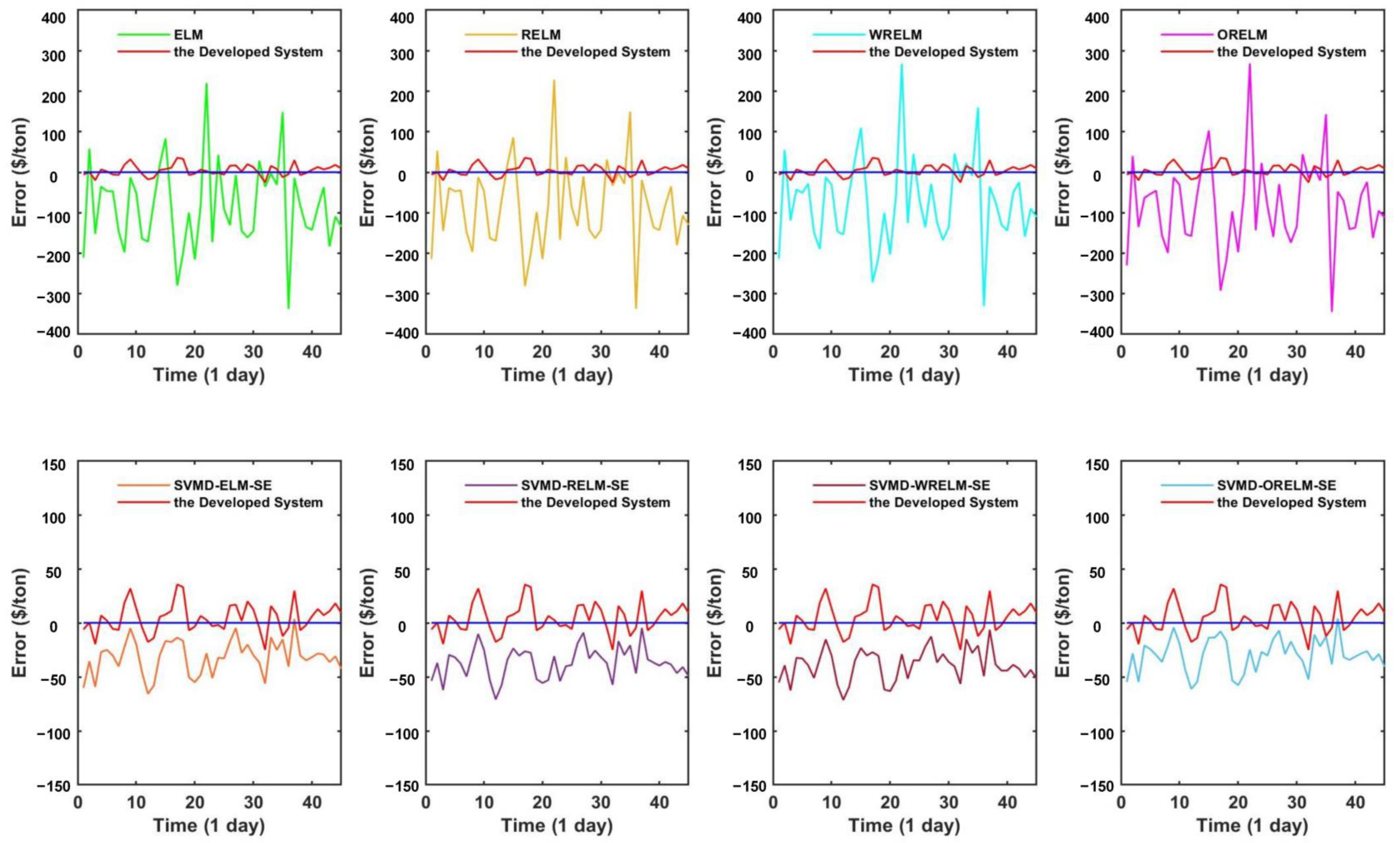
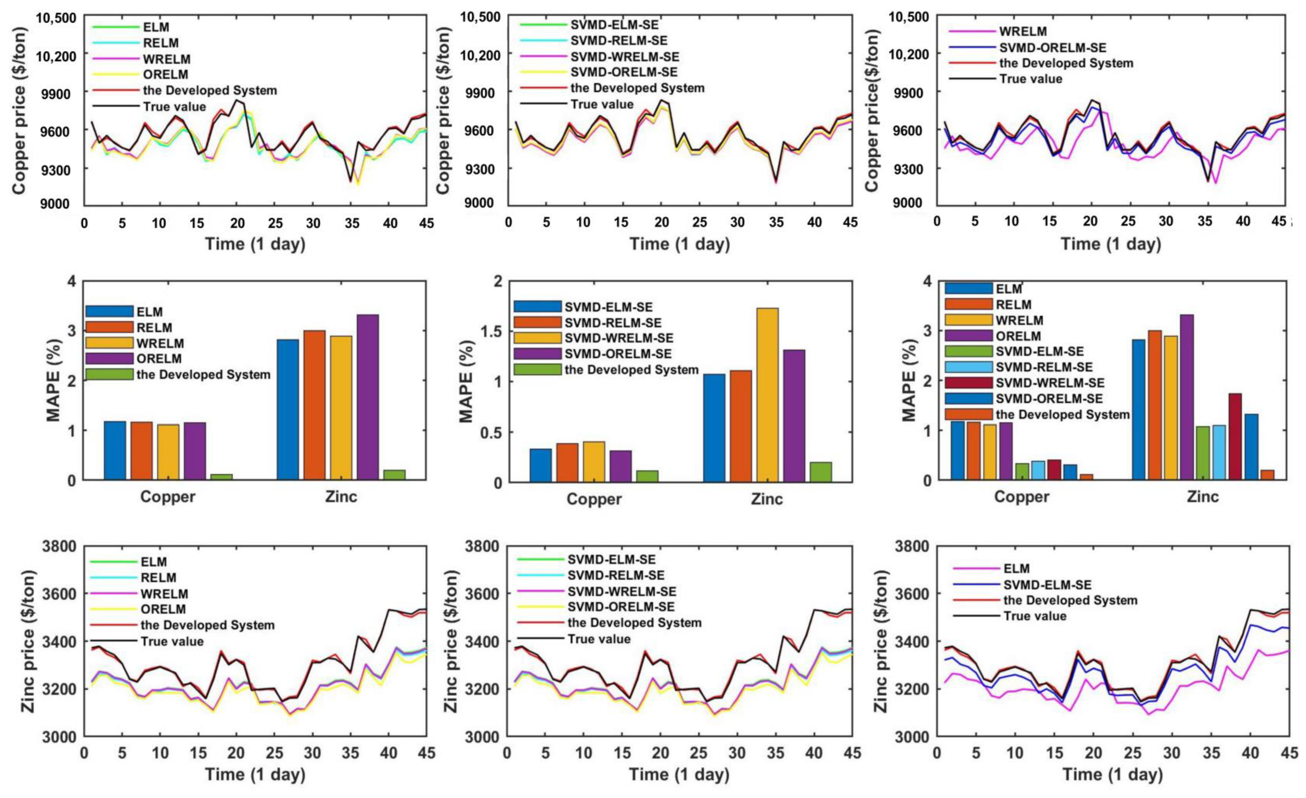
In this section, the point forecasting comparison results among the proposed forecasting system and some typical benchmark models are shown in Table 4 and Figure 2 and Figure 3, where the boldly marked value means the corresponding model achieves the best results in the specific evaluation index, showing that the developed forecasting system performs best among all models.
Figure 4 shows the graphical forecasting results for dataset copper and zinc, respectively, both of which demonstrate that the forecasting lines of the developed forecasting system are closer to the observation lines than any other comparison. On top of that, the system developed in this study obtains the best MAPE value among all comparison models. The comparative analysis results are as follows:
- (a)
- The comparison of point prediction accuracy among the simple ensemble models with some single models. In this sub-session, several independent forecasting models are selected, mainly including ELM and three improved versions of ELM, i.e., RELM, WRELM, and ORELM. From Table 4, it is obvious to see that the forecasting accuracy of the simple ensemble models is stronger than that of the individual models. Taking dataset copper as an example, the WRELM obtains the most satisfying prediction prevision in individual models with the MAPE index value of 1.108749%. For the single model WRELM, other index values are , , , , . Concerning simple ensemble models in Experiment II, the SVMD-ORELM-SE has the best forecasting performance both in simple ensemble models and individual models, whose corresponding values are , , , , .
- (b)
- The comparison of point prediction accuracy between the designed system and single models. According to Table 4, it is obvious that the forecasting prevision of the designed system is stronger than those single models. For dataset copper, the model which has the highest accuracy in individual models is WRELM, and the corresponding index values are mentioned above in part (a). Compared to an individual model, the developed forecasting system has a great improvement, such as the MAPE value of 1.108479% and 0.118460% for WRELM and the proposed system, respectively. In addition to this, the other corresponding index values for the developed system are , , , , .
- (c)
- The comparison of point prediction accuracy between the proposed system and simple ensemble models. According to Table 4, taking dataset zinc as an example, the SVMD-ELM-SE achieves the most satisfying results in simple ensemble models with the corresponding index values of , , , , . Meanwhile, the Developed System index values are , , , , . Through the experimental results, there is no doubt that the prediction precision of the developed system is much better than those simple ensemble models.
Remark 2.
The most suitable prediction sub-predictor for each mode is selected with the lowest MRMIT index value to establish the developed forecasting system. Results of the developed system, the single models, and the simple ensemble models are compared, it is easy to conclude that simple ensemble methods are better than single models, the nonlinear ensemble mode is better than simple ensemble methods, and the system proposed in this study obtains the best results.
5.5. Experiment III: Ensemble Point Forecasting Based on the Optimal Model Selection Strategy
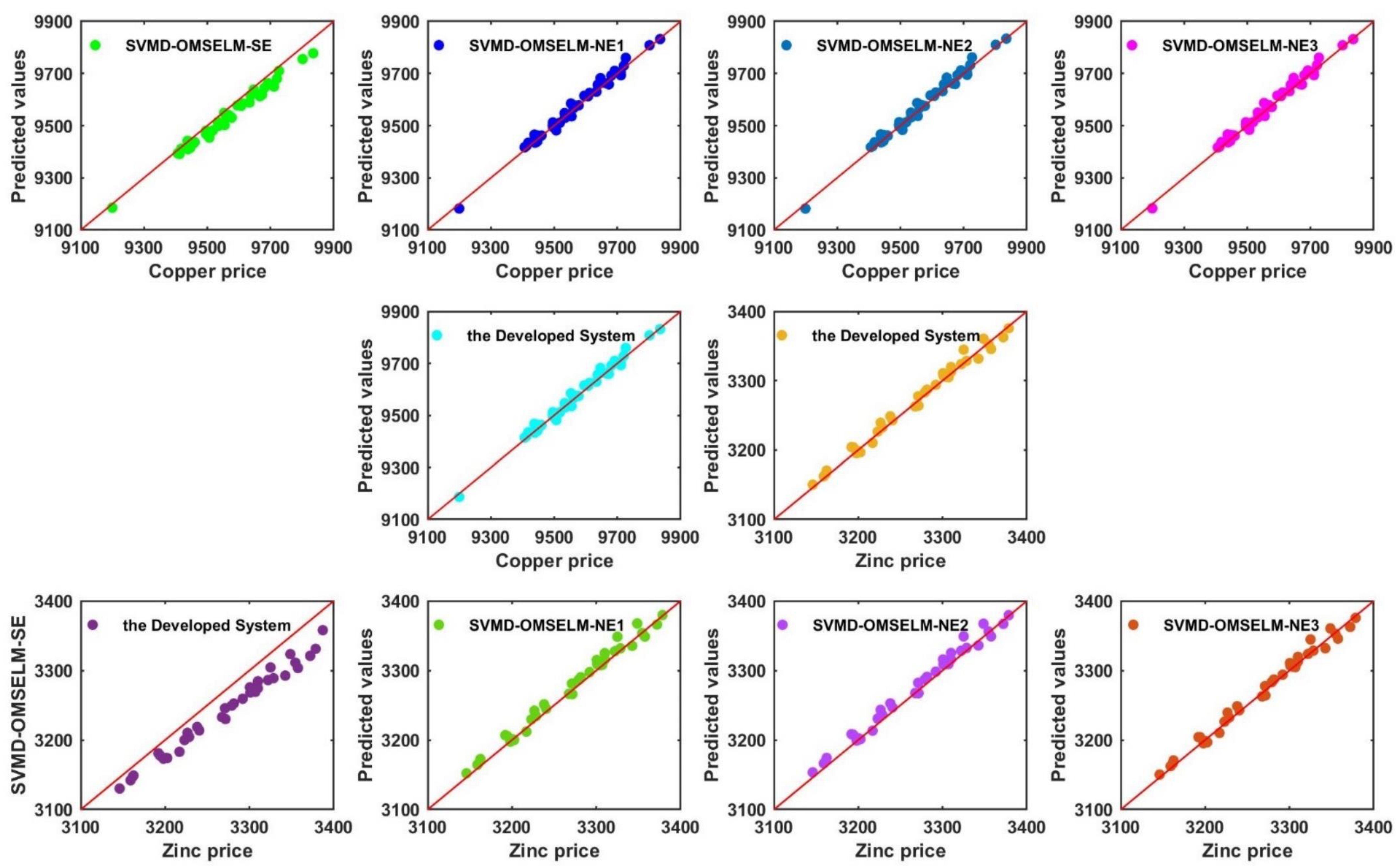
Experiment III is implemented to demonstrate the prediction precision of the proposed system and other hybrid models based on different ensemble strategies, such as simple ensemble (SE), ELM-nonlinear ensemble (NE1), RELM-nonlinear ensemble (NE2), WRELM-nonlinear ensemble (NE3) and ORELM-nonlinear ensemble. For the ensemble methods of the proposed system, we substituted the ORELM-nonlinear ensemble for using the simple ensemble, ELM-nonlinear ensemble, RELM-nonlinear ensemble, and WRELM-nonlinear ensemble to forecast the non-ferrous metal prices, in the meantime, the other involved approaches and parameters in the experiment maintain the identical with the system proposed in this study. The comparison results of each model are listed in Table 5, where SVMD meaning of SVMD decomposition, OMSELM represents the optimal model selection in the ELM series model for each decomposed mode, SE, and Nes are mentioned above, and the results are also presented in Figure 5 for providing a clear contrast.
- (a)
- The developed system is compared with the SVMD-OMSELM-SE model Table 5 displays that in the case of dataset copper, the developed system has a lower MAPE value than SVMD-OMSELM-SE, with values of 0.118469% and 0.310760%, which indicates that the developed system has better prediction precision. Moreover, for the developed system, the other evaluation criteria are mentioned above in Experiment II: (b). Corresponding to this is SVMD-OMSELM-SE, the corresponding indexes are , , , , respectively. From this, it is believed that the developed system is prominently superior to the SVMD-OMSELM-SE based on the five comprehensive evaluation indicators and it can be further concluded that ORELM nonlinear ensemble is better than the simple ensemble.
- (b)
- The developed system is compared with SVMD-OMSELM based on different nonlinear ensemble methods, such as RELM-nonlinear ensemble, WRELM-nonlinear ensemble, and ORELM-nonlinear ensemble. From Table 5, taking the dataset copper as an example, we can see that the best forecasting model among the SVMD-OMSELM based on three different nonlinear ensemble is SVMD-OMSELM-NE1, whose assessment indexes are , , , , , respectively. And the indexes of the proposed system are mentioned above specifically. By contrast, the developed system forecasting results surpass SVMD-OMSELM-NE1, that’s to say, the proposed system has the best forecasting prevision.
Remark 3.
According to the prediction evaluation indexes of the dataset copper and zinc, it is obvious that the nonlinear ensemble achieves better results compared to the simple ensemble, and the ORELM nonlinear ensemble has the best prediction performance compared to the ELM nonlinear ensemble, RELM nonlinear ensemble, and WRELM nonlinear ensemble.
5.6. Experiment IV: Interval Forecasting
Uncertainty prediction of non-ferrous metals prices is highly correlated with the non-ferrous metals industry which can provide more information. The forecasting interval can quantify the uncertainty and potential risk of the non-ferrous metal market. Based on the point prediction of each sub-series, interval prediction is carried out to achieve the interval consisting of upper and lower bounds, and the result can be a better indicator of the market. As is known to all, ELM and RELM can double output the experimental results and get the upper and lower sections of the interval prediction, but WRELM and ORELM are difficult to achieve this, so the developed forecasting system can only independently predict the interval’s upper and lower bounds. The interval forecasting results of the developed system are displayed in Table 6 and Figure 6. Taking Copper as an example, the PICP is always 100.00 at the confidence level of 99%, 95%, and 90%, respectively, and the relevant PIAW is 190.713983, 955.486526 and 1912.229981, the PINAW is 0.300101, 1.503519 and 3.009016, Score is −3.814280, −95.548653 and −573.668994. Results of Dataset Zinc are also presented in Table 6. All the PICPs are 100.00, meaning that the interval prediction results are desirable.
Remark 4.
For the dataset copper and zinc, the developed system has a wonderful forecasting performance, with the interval forecasting index PICP equal to 100 at a confidence level of 0.01. As a result, the system developed in this study can perform desirable interval forecasting.
6. Discussion
In this part, five discussions are performed to deeper investigate the proposed system, including the forecasting stability, effectiveness, and significance, and the superiority of each module in the developed system. The following subsections cover these discussions.
6.1. Forecasting Stability
In this research, the novel point and interval forecasting system based on the optimal sub-predictor selection strategy discussed is successfully developed based on the ORELM nonlinear ensemble method. The above experiments mainly focus on the discussion of prediction accuracy and cannot demonstrate the effect of the developed system in terms of stability. Therefore, it is necessary to discuss forecasting stability to further verify its superiority. In comparative studies, variance is a common method to evaluate prediction consistency. Therefore, this study adopts the method of model prediction error to measure its prediction stability. The value of variance indicates the performance effect of model stability. The model prediction error variances involved in this paper are listed in Table A1. The proposed system obtains the minimum variance with the VAR value is 188.906506 and 70.112261 for datasets Copper and Zinc, respectively. Based on the results in Table A1, the designed system has the best predictive stability, followed by the simple ensemble model, and the single model has the worst stability. Furthermore, the ensemble mode not only improves the prediction accuracy of the model, but also enhances the prediction stability of the model.
6.2. Forecasting Effectiveness
To further demonstrate the superiority of the prediction system, FE is conducted to measure the prediction effectiveness. And the higher the FE value, the more accurate the predicted performance of the model is. The FE values in Table A2 reveal that: (a) for copper and zinc datasets, the FE1 values of the proposed system are 0.998815 and 0.997916, and the FE2 values are 0.997887 and 0.996500, respectively; (b) In all instances, the FE values of the system proposed in this study is higher than that of the benchmark model. Therefore, the proposed prediction system surpasses all the comparison models; (c) Looking at the results in Table A2, the designed system is superior to the simple ensemble models, and the simple ensemble model is superior to the single models. In addition, the simple ensemble model based on model selection is better than a simple ensemble model without model selection.
6.3. Statistical Significance
Significance tests are designed to indicate whether the differences between the developed system and the comparison models in experiments are significant. There are many methods to test the validity of models, among which Diebold-Mariano (DM) statistic is a general index to measure the model’s statistical significance. For the convenience of testing, the developed system is used as a standard, and the correlation model is used as a compared model. Overall, the null hypothesis indicates that the prediction performance of the developed system is as valid as the prediction performance of the comparison model. On the contrary, the alternative hypothesis implies that the predictive power of the developed system is significantly different from the benchmarks. But as the forecast data sets grow, their test results can be wildly inflated. To overcome this shortcoming, Modified DM (MDM) hypothesis test is proposed. The first correction relies on , where stands for the multi-period advance forecast. Another improvement is to compare the DM with the critical value of the t-distribution from the test number -1degree. The DM and MDM test results between the developed system and other comparisons are presented in Table A3.
- (a)
- For dataset Copper, except , all the comparative models passed the test under . The residual model DM values are greater than , with the minimum DM value is 2.811426. This means the developed system has 99% probability to reject , that is to say, under 99% confidence interval, the developed system has excellent prediction accuracy. For degrees of freedom 44, taking dataset copper as an example, except , other P values are lower than the significance level . Of the remaining MDM-P values, the largest is , which indicates that the developed system has 99% probability to reject . However, at the significance level of , all the comparative models reject .
- (b)
- As for the comparative models of Zinc, 100% of the results passed the significance test of . Under different ensemble strategies, , , , , , , , , it shows that the proposed forecasting system has the best prediction ability. The results of the MDM hypothesis test show that besides the performance of SVMD-OMSELM-NE1 are , all the results are lower than , which demonstrates that the proposed forecasting has 99% probability to reject .
6.4. The Superiority of Each Module in the Developed System
To fully demonstrate the advantages of the developed system, the improvement degree between the developed system and the comparison models needs to be discussed. How each component works in the developed system should be quantified and analyzed. As a result, in this subsection, five metrics(, , , and defined as Equation (39) represents the percentage improvement in terms of MAE, RMSE, MAPE, IA, and TIC, respectively), were used to demonstrate the precision and validity of the developed system detailedly. On this basis, the detailed error improvement percentage of 15 pairs of models is calculated. As shown in Table A4, the percentage improvement value of each pair of models is greater than 0, and the forecasting prevision of the proposed strategy is also improved compared with the benchmark method.
Moreover, we can draw the following conclusions:
- (a)
- By comparing SVMD-OMSELM-SE and SVMD-ELM-SE, SVMD-OMSELM-SE and SVMD-RELM-SE, SVMD-OMSELM-SE and SVMD-WRELM-SE, SVMD-OMSELM-SE and SVMD-ORELM-SE, can prove the superiority of the newly introduced optimal model selection mode. And in the comparison between SVMD-OMSELM-SE and SVMD-WRELN-SE, model selection shows the best superiority, the , , , and index values on average are 30.8827%, 28.1601%, 30.9649%, 3.6435%, and 28.2820%, respectively. At the same time, by comparing SVMD-OMSELM-NE1 and SVMD-ELM-SE, SVMD-OMSELM-NE2 and SVMD-RELM-SE, SVMD-OMSELM-NE3 and SVMD-WRELM-SE, SVMD-OMSELM-NE4 and SVMD-ORELM-SE, can further prove that model selection is effective in improving the prediction system with nonlinear strategies. There is no doubt from Table A4 that under the nonlinear ensemble method, the comparison of SVMD-OMSELM-NE3 and SVMD-WRELM-SE, the optimal sub-predictor, has the best effect on point forecasting accuracy. On average the , , , and metrics are 77.9806%, 74.4655%, 77.8866%, 6.4755% and 74.5771%, respectively. In addition, it is reasonable to demonstrate the superiority of the nonlinear ensemble mode.
- (b)
- According to the improvement rates of the developed system with the SVMD-OMSELM-SE, SVMD-OMSELM-NE1, SVMD-OMSELM-NE2, and SVMD-OMSELM-NE3 models, the effectiveness of the ORELM nonlinear ensemble approach in the developed system is verified. On top of that, the ORELM nonlinear ensemble approach is a great improvement over a simple ensemble and on average the , , , and metrics are 71.5818%, 68.0750%, 71.4459%, 2.7481%, and 68.1724%.
- (c)
- The comparison of the developed system with SVMD-ELM-SE, SVMD-RELM-SE, and SVMD-ORELM-SE, respectively, not only validates the effectiveness of model selection but also clearly explains the prospective of the ORELM nonlinear ensemble mode.
In summary, all the metric values are positive, meaning that the system presented in this study outperforms the comparative methods in non-ferrous metal prediction due to the superiority of each module.
6.5. Comparison with Existing Models
In this section, we select four metal price prediction models from a recently published study for 2019 to 2022 as comparison models. These models include Du et al. [9], Guo et al. [33], Luo et al. [54], and Drachal et al. [55]. As can be seen from Table A5, the developed forecasting system in this paper is superior to the comparison models in prediction accuracy, prediction ability and generalization ability, in which the developed system obtains the lowest MAE, RMSE, MAPE, and TIC values and the largest IA values on non-ferrous metal price forecasting. On the other hand, from the theoretical point of view, the optimal sub-model selection strategy and nonlinear ensemble mode are proposed in the developed system, which can improve the prediction performance of the model. However, the model proposed by Du et al. [9], Guo et al. [33], Luo et al. [54], and Drachal et al. [55] ignores the significance of model selection and ensemble mode in metal price prediction and has certain limitations. In general, the developed forecasting system provides a new theoretical framework for metal price forecasting methods, which can obtain better prediction results by enjoying the optimal sub-model and nonlinear ensemble and can provide a reference for metal price forecasting and prediction research in related fields.
7. Conclusions
A reliable non-ferrous metal price prediction system can help decision makers to rationally manage metal mining, refining, and foreign trade, and effectively ensure the reliable operation of national industrial production. However, the existing research focus on the application of individual advanced models and neglect the in-depth analysis and mining of a certain type of model. In addition, as relatively advanced forecasting methods, sub-model selection strategy and ensemble mode are rarely involved in non-ferrous metals price forecasting, leading to poor forecasting results under some circumstances. Besides, the previous data pretreatment algorithms have the disadvantage of being difficult to determine the number of decomposition layers, which may play a crucial role in the final prediction precision. To bridge these research gaps, considering the inherent instability of the data and achieving accurate metal price prediction results, a novel point and interval non-ferrous metal prices forecasting system based on optimal sub-model selection strategy and nonlinear ensemble mode is proposed for non-ferrous metal prices futures market management in this study. The main conclusions of this study include:
- (1)
- Compared with other comparative models, the developed system can achieve better metal price forecasting performance due to the combination of different components, such as data decomposition techniques, sub-model selection strategy, and nonlinear ensemble methods. In addition, in this paper, the ELM, RELM, WRELM, and ORELM model are considered and analyzed, and the prediction result is better than the comparison models. Therefore, the in-depth analysis and mining of a certain type of model can be paid more attention to in the future;
- (2)
- The successive variational mode decomposition (SVMD) algorithm is introduced to determine the number of decomposed sub-sequences according to the intrinsic characteristics of the data, which can effectively reduce the occurrence of errors. Specifically, the SVMD data pretreatment algorithm can reduce the volatility and non-linearity of non-ferrous metal data by decomposing the original data into multiple sub-sequences, and improve the prediction performance;
- (3)
- Based on the proposed MRMIT index, the optimal predictor is selected for each decomposed sub-sequence, which enhances the prediction accuracy as well as expands the application scope of the forecasting system. The experimental results show that the model selection introduced into the non-ferrous metal price forecasting field is effective;
- (4)
- Compared with the single model, simple ensemble method, ELM, RELM, and WRELM nonlinear ensemble method, the proposed ORELM nonlinear ensemble mode has better forecasting precision and consistency, which verifies the validity of the novel nonlinear ensemble mode;
- (5)
- The developed system is superior to the comparative models in the non-ferrous metal trading market. For the dataset copper and zinc, the mean MAPE values of the developed system are 0.118469 and 0.203406, respectively. The interval forecasting results show that at the significance level of 0.01, PICP values are 100.000000 and 100.000000; PIAW values are 190.713983 and 65.090031, respectively; PINAW values are 0.300101 and 0.167758; SCORE values are −3.814280 and −1.301801, respectively. Therefore, the developed system in this paper is an effective complement to the existing non-ferrous metal price forecasting research framework, which is conducive to the operation and management of the non-ferrous metal market.
In addition, this study also has some policy implications and industrial applications, because the developed system can provide valuable information for non-ferrous metal producers, investors, regulators, and other participants, and can be used to estimate future short-term metal price forecasts, design bidding strategies and purchasing plans, conduct risk management, conduct financial analysis, and adjust relevant policies. First of all, a more effective metal price forecasting model can not only help the government and relevant departments to formulate better deregulation policies and pricing, but also improve market price transparency, help producers and investors adjust bidding strategies and change production and consumption schedules. Secondly, understanding the non-ferrous metal price model can not only help enterprise managers improve their pricing strategies, but also effectively adjust the future strategic plans of enterprises, deal with cooperation agreements with customers, and finally realize the sustained and stable operation of metal mining and improve the profitability of the company. Thirdly, the findings of this study provide a new experience to prove that model selection is of great significance in accurately predicting the price of nonferrous metals. On the one hand, it can improve the efficiency and accuracy of metal price forecasting and provide more information advantages for decision-makers; On the other hand, it can help public decision makers to formulate better laws and regulations to improve market rules.
Although the proposed system is a promising, applicable, and effective technique for the non-ferrous metal market, the proposed system also has some limitations that require further study. Specifically, this study only focuses on the problem of univariate prediction and does not take into account other factors affecting non-ferrous metals. Other factors, such as the black swan event, changes in the economic environment, supply and demand relations, international situation, and technological progress, among others, will also affect future price changes, which can be considered in future studies. Moreover, non-ferrous metals price forecasting under extreme volatility is still a challenging but meaningful task, which can be considered another future research direction. Besides, on account of the finite research scope, four candidate prediction sub-predictors of the ELM series are selected in this paper, while other prediction sub-models can be further discussed in future studies. In addition, the forecasting system and its ideas proposed in this paper can also be applied to wind speed forecasting [56], intermittent demand forecasting [57], tourism demand forecasting [58], stock prices forecasting [48], bioenergy power generation structure forecasting [59] and other fields.
Author Contributions
S.Y.: Conceptualization, software, methodology, writing—original draft preparation. W.Y.: supervision, formal analysis, funding acquisition, writing—review and editing. K.Z.: investigation, visualization, writing—reviewing and editing. Y.H.: supervision, funding acquisition, writing—review and editing. All authors have read and agreed to the published version of the manuscript.
Funding
This work supported by National Natural Science Foundation of China (Grant No. 72101138); Humanities and Social Science Fund of Ministry of Education of the People’s Republic of China (Grant No. 21YJCZH198); Shandong Provincial Natural Science Foundation, China (Grant No. ZR2021QG034, ZR2022QG036); Social Science Planning Project of Shandong Province (Grant No. 22DJJJ24); and Special Support for Post-doc Creative Funding in Shandong, China (Grant No. 202103018).
Data Availability Statement
Data can be found at: https://cn.investing.com (accessed on 1 July 2022).
Conflicts of Interest
The authors declare that there is no conflict of interest concerning the publication of this paper.
Appendix A

Table A1.
Results of prediction stability.
| Dataset | Model | VAR |
|---|---|---|
| Copper | ELM | 11,286.993097 |
| RELM | 11,336.186827 | |
| WRELM | 11,968.801480 | |
| ORELM | 12,181.008417 | |
| SVMD-ELM-SE | 252.066521 | |
| SVMD-RELM-SE | 212.343312 | |
| SVMD-WRELM-SE | 219.031314 | |
| SVMD-ORELM-SE | 243.856001 | |
| SVMD-OMSELM-SE | 244.223998 | |
| SVMD-OMSELM-NE1 | 191.637117 | |
| SVMD-OMSELM-NE2 | 197.689493 | |
| SVMD-OMSELM-NE3 | 197.740229 | |
| The Developed System | 188.906506 | |
| Zinc | ELM | 3215.968100 |
| RELM | 3329.516374 | |
| WRELM | 3251.063837 | |
| ORELM | 3779.192421 | |
| SVMD-ELM-SE | 321.593545 | |
| SVMD-RELM-SE | 339.918353 | |
| SVMD-WRELM-SE | 611.193976 | |
| SVMD-ORELM-SE | 384.366274 | |
| SVMD-OMSELM-SE | 319.900086 | |
| SVMD-OMSELM-NE1 | 77.863428 | |
| SVMD-OMSELM-NE2 | 79.968606 | |
| SVMD-OMSELM-NE3 | 83.227507 | |
| The Developed System | 70.112261 |
Table A2.
Results for the Forecasting effectiveness.
| Dataset | Model | FE1 | FE2 |
|---|---|---|---|
| Copper | ELM | 0.988279 | 0.980377 |
| RELM | 0.988383 | 0.980444 | |
| WRELM | 0.988913 | 0.980959 | |
| ORELM | 0.988470 | 0.980227 | |
| SVMD-ELM-SE | 0.996655 | 0.995058 | |
| SVMD-RELM-SE | 0.996126 | 0.994635 | |
| SVMD-WRELM-SE | 0.995917 | 0.994408 | |
| SVMD-ORELM-SE | 0.996873 | 0.995308 | |
| SVMD-OMSELM-SE | 0.996892 | 0.995328 | |
| SVMD-OMSELM-NE1 | 0.998795 | 0.997853 | |
| SVMD-OMSELM-NE2 | 0.998753 | 0.997750 | |
| SVMD-OMSELM-NE3 | 0.998756 | 0.997783 | |
| The Developed System | 0.998815 | 0.997887 | |
| Zinc | ELM | 0.971854 | 0.956776 |
| RELM | 0.969984 | 0.954638 | |
| WRELM | 0.971185 | 0.955986 | |
| ORELM | 0.966815 | 0.950374 | |
| SVMD-ELM-SE | 0.989278 | 0.984363 | |
| SVMD-RELM-SE | 0.988938 | 0.983902 | |
| SVMD-WRELM-SE | 0.982712 | 0.976083 | |
| SVMD-ORELM-SE | 0.986860 | 0.981534 | |
| SVMD-OMSELM-SE | 0.989290 | 0.984390 | |
| SVMD-OMSELM-NE1 | 0.997639 | 0.995927 | |
| SVMD-OMSELM-NE2 | 0.997529 | 0.995736 | |
| SVMD-OMSELM-NE3 | 0.997624 | 0.996060 | |
| The Developed System | 0.997966 | 0.996500 |
Table A3.
Results for the DM and MDM test.
| Dataset | Model | DM | MDM | MDM-P |
|---|---|---|---|---|
| Copper | ELM | 5.461142 | 5.400121 | 2.546700 × 10⁻⁶ |
| RELM | 5.372157 | 5.312131 | 3.418049 × 10⁻⁶ | |
| WRELM | 5.001746 | 4.945858 | 1.152746 × 10⁻⁵ | |
| ORELM | 4.994495 | 4.938688 | 1.180302 × 10⁻⁵ | |
| SVMD-ELM-SE | 5.866314 | 5.800767 | 6.617725 × 10⁻⁷ | |
| SVMD-RELM-SE | 7.544789 | 7.460487 | 2.430326 × 10⁻⁹ | |
| SVMD-WRELM-SE | 7.917927 | 7.829456 | 7.098852 × 10⁻¹⁰ | |
| SVMD-ORELM-SE | 5.466845 | 5.405761 | 2.499056 × 10⁻⁶ | |
| SVMD-OMSELM-SE | 5.450666 | 5.389763 | 2.636570 × 10⁻⁶ | |
| SVMD-OMSELM-NE1 | 1.313350 | 1.298675 | 2.008207 × 10⁻¹ | |
| SVMD-OMSELM-NE2 | 2.969721 | 2.936539 | 5.262398 × 10⁻³ | |
| SVMD-OMSELM-NE3 | 2.811426 | 2.780013 | 7.967935 × 10⁻³ | |
| The Developed System | ||||
| Zinc | ELM | 6.307776 | 6.237296 | 1.510907 × 10⁻⁷ |
| RELM | 6.553817 | 6.480588 | 6.624987 × 10⁻⁸ | |
| WRELM | 6.392678 | 6.321249 | 1.136804 × 10⁻⁷ | |
| ORELM | 6.757235 | 6.681733 | 3.352119 × 10⁻⁸ | |
| SVMD-ELM-SE | 6.478134 | 6.405751 | 8.537268 × 10⁻⁸ | |
| SVMD-RELM-SE | 6.462337 | 6.390130 | 9.001363 × 10⁻⁸ | |
| SVMD-WRELM-SE | 7.373679 | 7.291289 | 4.286835 × 10⁻⁹ | |
| SVMD-ORELM-SE | 7.190442 | 7.110099 | 7.886491 × 10⁻⁹ | |
| SVMD-OMSELM-SE | 6.481959 | 6.409533 | 8.428536 × 10⁻⁸ | |
| SVMD-OMSELM-NE1 | 2.581770 | 2.552922 | 1.422681 × 10⁻² | |
| SVMD-OMSELM-NE2 | 3.217786 | 3.181831 | 2.683958 × 10⁻³ | |
| SVMD-OMSELM-NE3 | 3.424765 | 3.386498 | 1.500084 × 10⁻³ | |
| The Developed System | - | - | - |
Table A4.
Results of the improvement percentage.
| Copper | Zinc | Average | Copper | Zinc | Average | Copper | Zinc | Average | Copper | Zinc | Average | Copper | Zinc | Average | |
|---|---|---|---|---|---|---|---|---|---|---|---|---|---|---|---|
| SVMD-OMSELM-SE vs. | SVMD-OMSELM-SE vs. | SVMD-OMSELM-NE3 vs. | The Developed System vs. | The Developed System vs. | |||||||||||
| SVMD-ELM-SE | SVMD-ORELM-SE | SVMD-WRELM-SE | SVMD-OMSELM-NE1 | SVMD-ELM-SE | |||||||||||
| MAE | 7.0678 | 0.1133 | 3.5906 | 0.6295 | 18.3435 | 9.4865 | 69.5705 | 86.3908 | 77.9806 | 1.6528 | 13.612 | 7.6324 | 64.6517 | 81.2215 | 72.9366 |
| RMSE | 6.0928 | 0.1427 | 3.1178 | 0.522 | 16.7136 | 8.6178 | 63.9291 | 85.0019 | 74.4655 | 1.5392 | 13.4568 | 7.498 | 59.6162 | 79.1837 | 69.3999 |
| MAPE | 7.1045 | 0.1107 | 3.6076 | 0.6286 | 18.4909 | 9.5597 | 69.5174 | 86.2559 | 77.8866 | 1.6997 | 13.8313 | 7.7655 | 64.5859 | 81.0294 | 72.8076 |
| IA | 0.2594 | 0.0125 | 0.136 | 0.0223 | 1.7355 | 0.8789 | 2.8186 | 10.1325 | 6.4755 | 9.78 × 10⁻⁷ | 0.0506 | 0.0302 | 1.9535 | 3.8195 | 2.8865 |
| TIC | 6.1041 | 0.1433 | 3.1237 | 0.5231 | 16.816 | 8.6695 | 64.0141 | 85.1402 | 74.5771 | 1.5372 | 13.4172 | 7.4772 | 59.6936 | 79.3012 | 69.4974 |
| SVMD-OMSELM-SE vs. | SVMD-OMSELM-NE1 vs. | The Developed System vs. | The Developed System vs. | The Developed System vs. | |||||||||||
| SVMD-RELM-SE | SVMD-ELM-SE | SVMD-ORELM-SE | SVMD-OMSELM-NE2 | SVMD-RELM-SE | |||||||||||
| MAE | 19.706 | 3.2039 | 11.455 | 64.0577 | 78.2626 | 71.1601 | 62.2028 | 84.6488 | 73.4258 | 4.9404 | 17.2478 | 11.0941 | 69.4589 | 81.8025 | 75.6307 |
| RMSE | 16.1141 | 3.1622 | 9.6381 | 58.9848 | 75.9469 | 67.4659 | 57.2205 | 82.638 | 69.9293 | 5.9168 | 17.0816 | 11.4992 | 63.9257 | 79.8131 | 71.8694 |
| MAPE | 19.7734 | 3.1771 | 11.4753 | 63.9736 | 77.9843 | 70.9789 | 62.1171 | 84.5201 | 73.3186 | 4.9698 | 17.672 | 11.3209 | 69.4156 | 81.6117 | 75.5137 |
| IA | 0.8259 | 0.2896 | 0.5577 | 1.9435 | 3.767 | 2.8552 | 1.7123 | 5.608 | 3.6601 | 0.0426 | 0.0704 | 0.0565 | 2.5295 | 4.1071 | 3.3183 |
| TIC | 16.147 | 3.1800 | 9.6635 | 59.0643 | 76.0937 | 67.579 | 57.2978 | 82.7572 | 70.0275 | 5.9086 | 17.0352 | 11.4719 | 64.0047 | 79.9307 | 71.9677 |
| SVMD-OMSELM-SE vs. | SVMD-OMSELM-NE2 vs. | The Developed System vs. | The Developed System vs. | The Developed System vs. | |||||||||||
| SVMD-WRELM-SE | SVMD-RELM-SE | SVMD-OMSELM-SE | SVMD-OMSELM-NE3 | SVMD-WRELM-SE | |||||||||||
| MAE | 23.8358 | 37.9296 | 30.8827 | 67.8716 | 78.0097 | 72.9407 | 61.9634 | 81.2002 | 71.5818 | 4.7954 | 14.256 | 9.5257 | 71.0297 | 88.3309 | 79.6803 |
| RMSE | 20.0512 | 36.2689 | 28.1601 | 61.657 | 75.6545 | 68.6558 | 56.996 | 79.1539 | 68.0750 | 4.6844 | 11.4193 | 8.0518 | 65.6188 | 86.7146 | 76.1667 |
| MAPE | 23.8805 | 38.0494 | 30.9649 | 67.8161 | 77.6646 | 72.7404 | 61.8775 | 81.0083 | 71.4429 | 4.8025 | 14.3966 | 9.5996 | 70.9813 | 88.2345 | 79.6079 |
| IA | 1.1447 | 6.1422 | 3.6435 | 2.4858 | 4.0338 | 3.2598 | 1.6896 | 3.8065 | 2.7481 | 0.0342 | 0.0454 | 0.0398 | 2.8537 | 10.1825 | 6.5181 |
| TIC | 20.0912 | 36.4829 | 28.2870 | 61.7443 | 75.8099 | 68.7771 | 57.0733 | 79.2715 | 68.1724 | 4.6786 | 11.3981 | 8.0383 | 65.6978 | 86.8339 | 76.2658 |
Table A5.
Comparison with existing models.
| Dataset | Model | MAE | RMSE | MAPE(%) | IA | TIC |
|---|---|---|---|---|---|---|
| Copper | Model proposed by [54] | 344.220000 | 421.454000 | 5.292000 | X | 0.032000 |
| Model proposed by [33] | 49.650600 | 74.677200 | 0.943100 | 0.988200 | X | |
| The Developed system | 11.332665 | 14.359648 | 0.118469 | 0.996536 | 0.000751 | |
| Zinc | Model proposed by [9] | 11.691300 | 14.611400 | 0.435800 | 0.999600 | X |
| Model proposed by [55] | 85.700000 | 112.000000 | X | X | X | |
| The Developed system | 6.757693 | 8.351136 | 0.203406 | 0.998478 | 0.001260 |
Note: X indicates that the author did not use such an indicator.
References
- Zhong, M.; He, R.; Chen, J.; Huang, J. Time-Varying Effects of International Nonferrous Metal Price Shocks on China’s Industrial Economy. Phys. A Stat. Mech. Its Appl. 2019, 528, 121299. [Google Scholar] [CrossRef]
- Liu, D.; Li, Z. Gold Price Forecasting and Related Influence Factors Analysis Based on Random Forest. In Proceedings of the Advances in Intelligent Systems and Computing; Springer: Singapore, 2017. [Google Scholar]
- Wang, J.; Hu, M.; Rodrigues, J.F.D. The Evolution and Driving Forces of Industrial Aggregate Energy Intensity in China: An Extended Decomposition Analysis. Appl. Energy 2018, 228, 2195–2206. [Google Scholar] [CrossRef]
- He, K.; Lu, X.; Zou, Y.; Keung Lai, K. Forecasting Metal Prices with a Curvelet Based Multiscale Methodology. Resour. Policy 2015, 45, 144–150. [Google Scholar] [CrossRef]
- Brown, P.P.; Hardy, N. Forecasting Base Metal Prices with the Chilean Exchange Rate. Resour. Policy 2019, 62, 256–281. [Google Scholar] [CrossRef]
- Fernandez, V. Copper Mining in Chile and Its Regional Employment Linkages. Resour. Policy 2021, 70, 101173. [Google Scholar] [CrossRef]
- Sánchez Lasheras, F.; de Cos Juez, F.J.; Suárez Sánchez, A.; Krzemień, A.; Riesgo Fernández, P. Forecasting the COMEX Copper Spot Price by Means of Neural Networks and ARIMA Models. Resour. Policy 2015, 45, 37–43. [Google Scholar] [CrossRef]
- Baur, D.G.; Smales, L.A. Hedging Geopolitical Risk with Precious Metals. J. Bank. Financ. 2020, 117, 105823. [Google Scholar] [CrossRef]
- Du, P.; Wang, J.; Yang, W.; Niu, T. Point and Interval Forecasting for Metal Prices Based on Variational Mode Decomposition and an Optimized Outlier-Robust Extreme Learning Machine. Resour. Policy 2020, 69, 101881. [Google Scholar] [CrossRef]
- Torres, J.L.; García, A.; De Blas, M.; De Francisco, A. Forecast of Hourly Average Wind Speed with ARMA Models in Navarre (Spain). Sol. Energy 2005, 79, 65–77. [Google Scholar] [CrossRef]
- Aasim; Singh, S.N.; Mohapatra, A. Repeated Wavelet Transform Based ARIMA Model for Very Short-Term Wind Speed Forecasting. Renew. Energy 2019, 136, 758–768. [Google Scholar] [CrossRef]
- Louka, P.; Galanis, G.; Siebert, N.; Kariniotakis, G.; Katsafados, P.; Pytharoulis, I.; Kallos, G. Improvements in Wind Speed Forecasts for Wind Power Prediction Purposes Using Kalman Filtering. J. Wind Eng. Ind. Aerodyn. 2008, 96, 2348–2362. [Google Scholar] [CrossRef] [Green Version]
- Kriechbaumer, T.; Angus, A.; Parsons, D.; Rivas Casado, M. An Improved Wavelet-ARIMA Approach for Forecasting Metal Prices. Resour. Policy 2014, 39, 32–41. [Google Scholar] [CrossRef] [Green Version]
- Gangopadhyay, K.; Jangir, A.; Sensarma, R. Forecasting the Price of Gold: An Error Correction Approach. IIMB Manag. Rev. 2016, 28, 6–12. [Google Scholar] [CrossRef] [Green Version]
- Chen, Y.; He, K.; Zhang, C. A Novel Grey Wave Forecasting Method for Predicting Metal Prices. Resour. Policy 2016, 49, 323–331. [Google Scholar] [CrossRef]
- Hao, Y.; Tian, C.; Wu, C. Modelling of Carbon Price in Two Real Carbon Trading Markets. J. Clean. Prod. 2020, 244, 118556. [Google Scholar] [CrossRef]
- Niu, X.; Wang, J. A Combined Model Based on Data Preprocessing Strategy and Multi-Objective Optimization Algorithm for Short-Term Wind Speed Forecasting. Appl. Energy 2019, 241, 519–539. [Google Scholar] [CrossRef]
- Zhang, H.; Nguyen, H.; Vu, D.A.; Bui, X.N.; Pradhan, B. Forecasting Monthly Copper Price: A Comparative Study of Various Machine Learning-Based Methods. Resour. Policy 2021, 73, 102189. [Google Scholar] [CrossRef]
- Fan, X.; Wang, L.; Li, S. Predicting Chaotic Coal Prices Using a Multi-Layer Perceptron Network Model. Resour. Policy 2016, 50, 86–92. [Google Scholar] [CrossRef]
- Mustaffa, Z.; Yusof, Y. Inter Related Metal Price Prediction Based on EABC-LSSVM. In Proceedings of the 2012 International Conference on Computer and Information Science, ICCIS 2012—A Conference of World Engineering, Science and Technology Congress, ESTCON 2012—Conference Proceedings, Kuala Lumpur, Malaysia, 12-14 June 2012. [Google Scholar]
- Liu, Y.; Yang, C.; Huang, K.; Gui, W. Non-Ferrous Metals Price Forecasting Based on Variational Mode Decomposition and LSTM Network. Knowl. Based Syst. 2020, 188, 105006. [Google Scholar] [CrossRef]
- Qiu, X.; Ren, Y.; Suganthan, P.N.; Amaratunga, G.A.J. Empirical Mode Decomposition Based Ensemble Deep Learning for Load Demand Time Series Forecasting. Appl. Soft Comput. J. 2017, 54, 246–255. [Google Scholar] [CrossRef]
- Aly, H.H.H. An Intelligent Hybrid Model of Neuro Wavelet, Time Series and Recurrent Kalman Filter for Wind Speed Forecasting. Sustain. Energy Technol. Assess. 2020, 41, 100802. [Google Scholar] [CrossRef]
- Cheng, H.; Ding, X.; Zhou, W.; Ding, R. A Hybrid Electricity Price Forecasting Model with Bayesian Optimization for German Energy Exchange. Int. J. Electr. Power Energy Syst. 2019, 110, 653–666. [Google Scholar] [CrossRef]
- Niu, H.; Xu, K.; Liu, C. A Decomposition-Ensemble Model with Regrouping Method and Attention-Based Gated Recurrent Unit Network for Energy Price Prediction. Energy 2021, 231, 120941. [Google Scholar] [CrossRef]
- Jiang, H.; Luo, S.; Dong, Y. Simultaneous Feature Selection and Clustering Based on Square Root Optimization. Eur. J. Oper. Res. 2021, 289, 214–231. [Google Scholar] [CrossRef]
- Zhu, B.; Ye, S.; Wang, P.; Chevallier, J.; Wei, Y.M. Forecasting Carbon Price Using a Multi-Objective Least Squares Support Vector Machine with Mixture Kernels. J. Forecast. 2022, 41, 100–117. [Google Scholar] [CrossRef]
- Jiang, H.; Tao, C.; Dong, Y.; Xiong, R. Robust Low-Rank Multiple Kernel Learning with Compound Regularization. Eur. J. Oper. Res. 2021, 295, 634–647. [Google Scholar] [CrossRef]
- Hao, Y.; Niu, X.; Wang, J. Impacts of Haze Pollution on China’s Tourism Industry: A System of Economic Loss Analysis. J. Environ. Manag. 2021, 295, 113051. [Google Scholar] [CrossRef]
- Wang, C.; Zhang, S.; Xiao, L.; Fu, T. Wind Speed Forecasting Based on Multi-Objective Grey Wolf Optimisation Algorithm, Weighted Information Criterion, and Wind Energy Conversion System: A Case Study in Eastern China. Energy Convers. Manag. 2021, 243, 114402. [Google Scholar] [CrossRef]
- Liu, Q.; Liu, M.; Zhou, H.; Yan, F. A Multi-Model Fusion Based Non-Ferrous Metal Price Forecasting. Resour. Policy 2022, 77, 102714. [Google Scholar] [CrossRef]
- Du, P.; Guo, J.; Sun, S.; Wang, S.; Wu, J. Multi-Step Metal Prices Forecasting Based on a Data Preprocessing Method and an Optimized Extreme Learning Machine by Marine Predators Algorithm. Resour. Policy 2021, 74, 102335. [Google Scholar] [CrossRef]
- Guo, H.; Wang, J.; Li, Z.; Lu, H.; Zhang, L. A Non-Ferrous Metal Price Ensemble Prediction System Based on Innovative Combined Kernel Extreme Learning Machine and Chaos Theory. Resour. Policy 2022, 79, 102975. [Google Scholar] [CrossRef]
- Wang, C.; Zhang, X.; Wang, M.; Lim, M.K.; Ghadimi, P. Predictive Analytics of the Copper Spot Price by Utilizing Complex Network and Artificial Neural Network Techniques. Resour. Policy 2019, 63, 101414. [Google Scholar] [CrossRef]
- Liu, C.; Hu, Z.; Li, Y.; Liu, S. Forecasting Copper Prices by Decision Tree Learning. Resour. Policy 2017, 52, 427–434. [Google Scholar] [CrossRef]
- Hussein, S.F.M.; Shah, M.B.N.; Jalal, M.R.A.; Abdullah, S.S. Gold Price Prediction Using Radial Basis Function Neural Network. In Proceedings of the 2011 4th International Conference on Modeling, Simulation and Applied Optimization, ICMSAO 2011, Kuala Lumpur, Malaysia, 19–21 April 2011. [Google Scholar]
- Li, B. Research on WNN Modeling for Gold Price Forecasting Based on Improved Artificial Bee Colony Algorithm. Comput. Intell. Neurosci. 2014, 2014, 1–10. [Google Scholar] [CrossRef] [Green Version]
- Liu, K.; Cheng, J.; Yi, J. Copper Price Forecasted by Hybrid Neural Network with Bayesian Optimization and Wavelet Transform. Resour. Policy 2022, 75, 102520. [Google Scholar] [CrossRef]
- Wang, J.; Li, H.; Wang, Y.; Lu, H. A Hesitant Fuzzy Wind Speed Forecasting System with Novel Defuzzification Method and Multi-Objective Optimization Algorithm. Expert Syst. Appl. 2021, 168, 114364. [Google Scholar] [CrossRef]
- Manickavasagam, J.; Visalakshmi, S.; Apergis, N. A Novel Hybrid Approach to Forecast Crude Oil Futures Using Intraday Data. Technol. Forecast. Soc. Chang. 2020, 158, 120126. [Google Scholar] [CrossRef]
- Hao, Y.; Zhou, Y.; Gao, J.; Wang, J. A Novel Air Pollutant Concentration Prediction System Based on Decomposition-Ensemble Mode and Multi-Objective Optimization for Environmental System Management. Systems 2022, 10, 139. [Google Scholar] [CrossRef]
- Deng, S.; Zhu, Y.; Duan, S.; Fu, Z.; Liu, Z. Stock Price Crash Warning in the Chinese Security Market Using a Machine Learning-Based Method and Financial Indicators. Systems 2022, 10, 108. [Google Scholar] [CrossRef]
- Lorenzo-Espejo, A.; Muñuzuri, J.; Guadix, J.; Escudero-Santana, A. A Hybrid Metaheuristic for the Omnichannel Multiproduct Inventory Replenishment Problem. J. Theor. Appl. Electron. Commer. Res. 2022, 17, 476–492. [Google Scholar] [CrossRef]
- Andrade, A.D.O.; Marques, L.G.; Resende, O. Prediction and Visualisation of SICONV Project Profiles Using Machine Learning. Systems 2022, 10, 252. [Google Scholar]
- Zhao, Y.; Li, Y.; Feng, C.; Gong, C.; Tan, H. Early Warning of Systemic Financial Risk of Local Government Implicit Debt Based on BP Neural Network Model. Systems 2022, 10, 207. [Google Scholar] [CrossRef]
- Zhang, L.; Wang, J.; Liu, Z. What Should Lenders Be More Concerned About? Developing A Profit-Driven Loan Default Prediction Model. Expert Syst. Appl. 2022, 213, 118938. [Google Scholar] [CrossRef]
- Lee, C.; Xu, X.; Lin, C.C. Using Online User-Generated Reviews to Predict Offline Box-Office Sales and Online DVD Store Sales in the O2O Era. J. Theor. Appl. Electron. Commer. Res. 2019, 14, 68–83. [Google Scholar] [CrossRef] [Green Version]
- Cheng, C.; Tsai, M.; Chang, C. A Time Series Model Based on Deep Learning and Integrated Indicator Selection Method for Forecasting Stock Prices and Evaluating Trading Profits. Systems 2022, 10, 243. [Google Scholar] [CrossRef]
- Febres, G.L.; Gershenson, C. A Deterministic–Statistical Hybrid Forecast Model: The Future of the COVID-19 Contagious Process in Several Regions of Mexico. Systems 2022, 10, 138. [Google Scholar] [CrossRef]
- Dragomiretskiy, K.; Zosso, D. Variational Mode Decomposition. IEEE Trans. Signal Process. 2014, 62, 531–544. [Google Scholar] [CrossRef]
- Nazari, M.; Sakhaei, S.M. Successive Variational Mode Decomposition. Signal Process. 2020, 174, 107610. [Google Scholar] [CrossRef]
- Huang, G.B.; Zhou, H.; Ding, X.; Zhang, R. Extreme Learning Machine for Regression and Multiclass Classification. IEEE Trans. Syst. Man Cybern. Part B Cybern. 2012, 42, 513–529. [Google Scholar] [CrossRef] [Green Version]
- Zhang, K.; Luo, M. Outlier-Robust Extreme Learning Machine for Regression Problems. Neurocomputing 2015, 151, 1519–1527. [Google Scholar] [CrossRef]
- Luo, H.; Wang, D.; Cheng, J.; Wu, Q. Multi-Step-Ahead Copper Price Forecasting Using a Two-Phase Architecture Based on an Improved LSTM with Novel Input Strategy and Error Correction. Resour. Policy 2022, 79, 102962. [Google Scholar] [CrossRef]
- Drachal, K. Forecasting Prices of Selected Metals with Bayesian Data-Rich Models. Resour. Policy 2019, 64, 101528. [Google Scholar] [CrossRef]
- Yang, W.; Hao, M.; Hao, Y. Innovative Ensemble System Based on Mixed Frequency Modeling for Wind Speed Point and Interval Forecasting. Inf. Sci. 2023, 622, 560–586. [Google Scholar] [CrossRef]
- Zhuang, X.; Yu, Y.; Chen, A. A Combined Forecasting Method for Intermittent Demand Using the Automotive Aftermarket Data. Data Sci. Manag. 2022, 5, 43–56. [Google Scholar] [CrossRef]
- Yang, Y.; Guo, J.; Sun, S. Tourism Demand Forecasting and Tourists’ Search Behavior: Evidence from Segmented Baidu Search Volume. Data Sci. Manag. 2021, 4, 1–9. [Google Scholar] [CrossRef]
- Zhang, K.; Yin, K.; Yang, W. Predicting Bioenergy Power Generation Structure Using a Newly Developed Grey Compositional Data Model: A Case Study in China. Renew. Energy 2022, 198, 695–711. [Google Scholar] [CrossRef]
Figure 1.
Flowchart of the point and interval forecasting system.
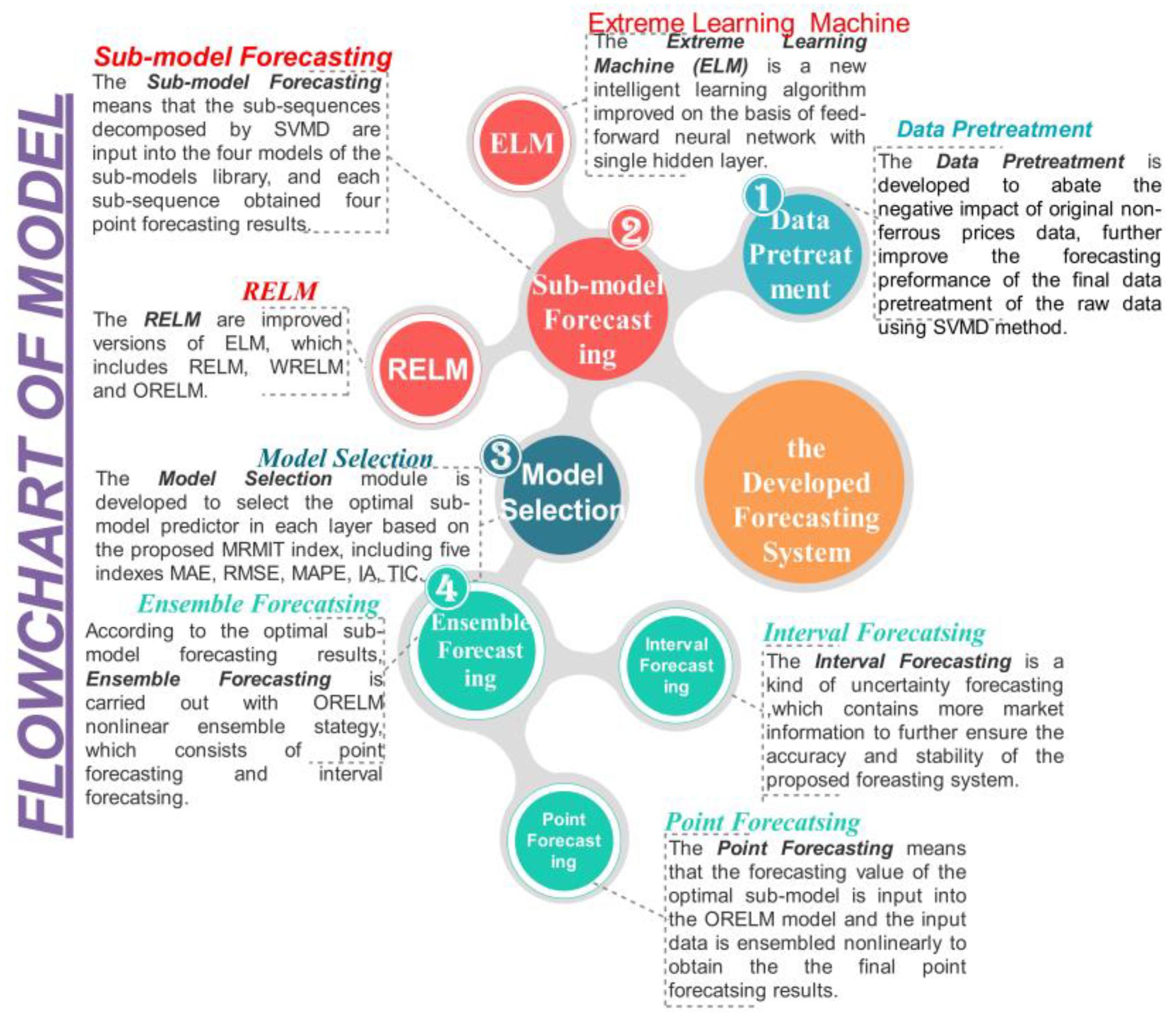
Figure 2.
Results of the developed system and some typical benchmark models for Dataset Copper.

Figure 3.
Results of the developed system and some typical benchmark models for Dataset Zinc.
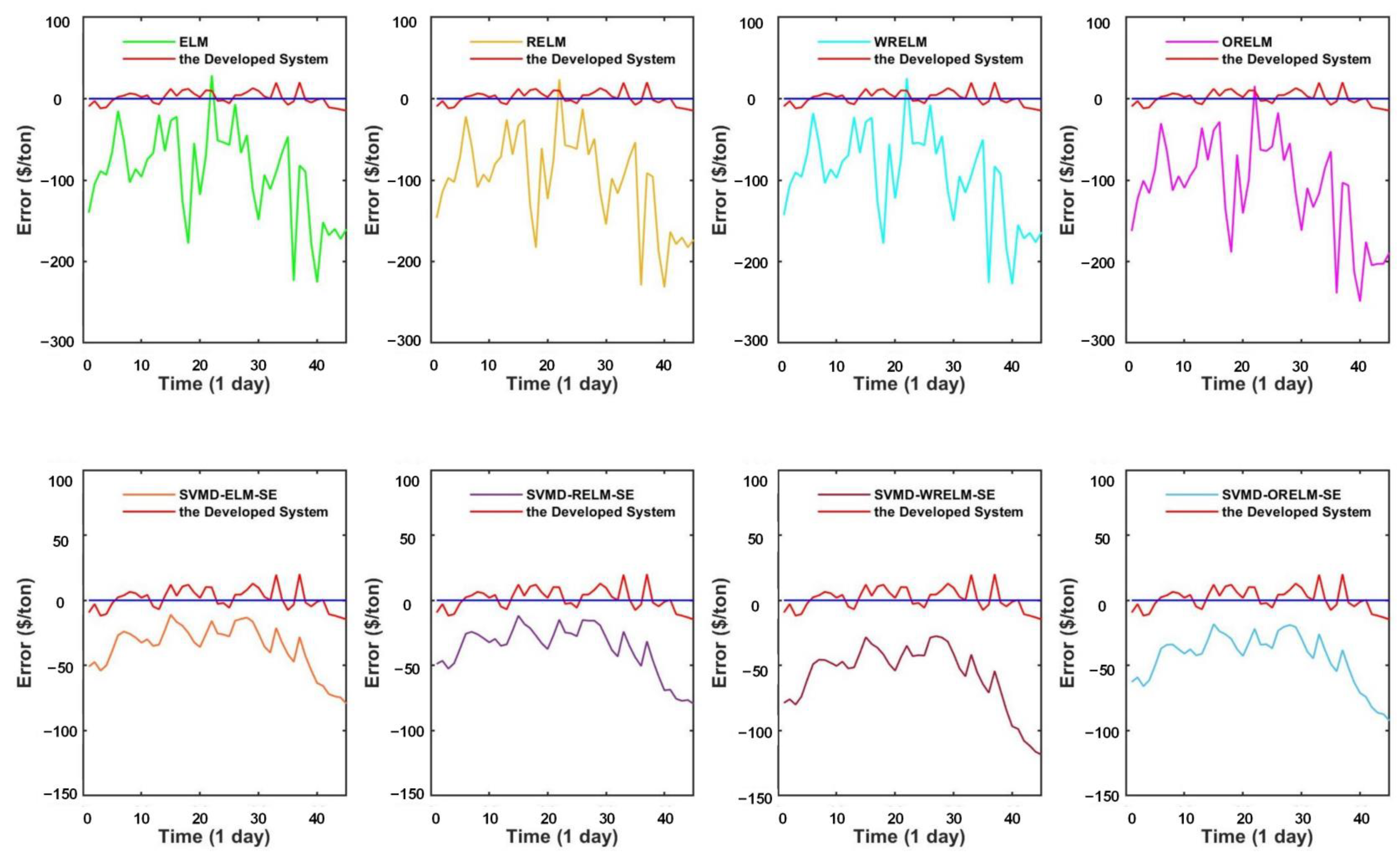
Figure 4.
The prediction results of two observation sites in Experiment II.

Figure 5.
Prediction results with different ensemble methods considered in Experiment III.

Figure 6.
Interval forecasting results for dataset copper and zinc price prediction.
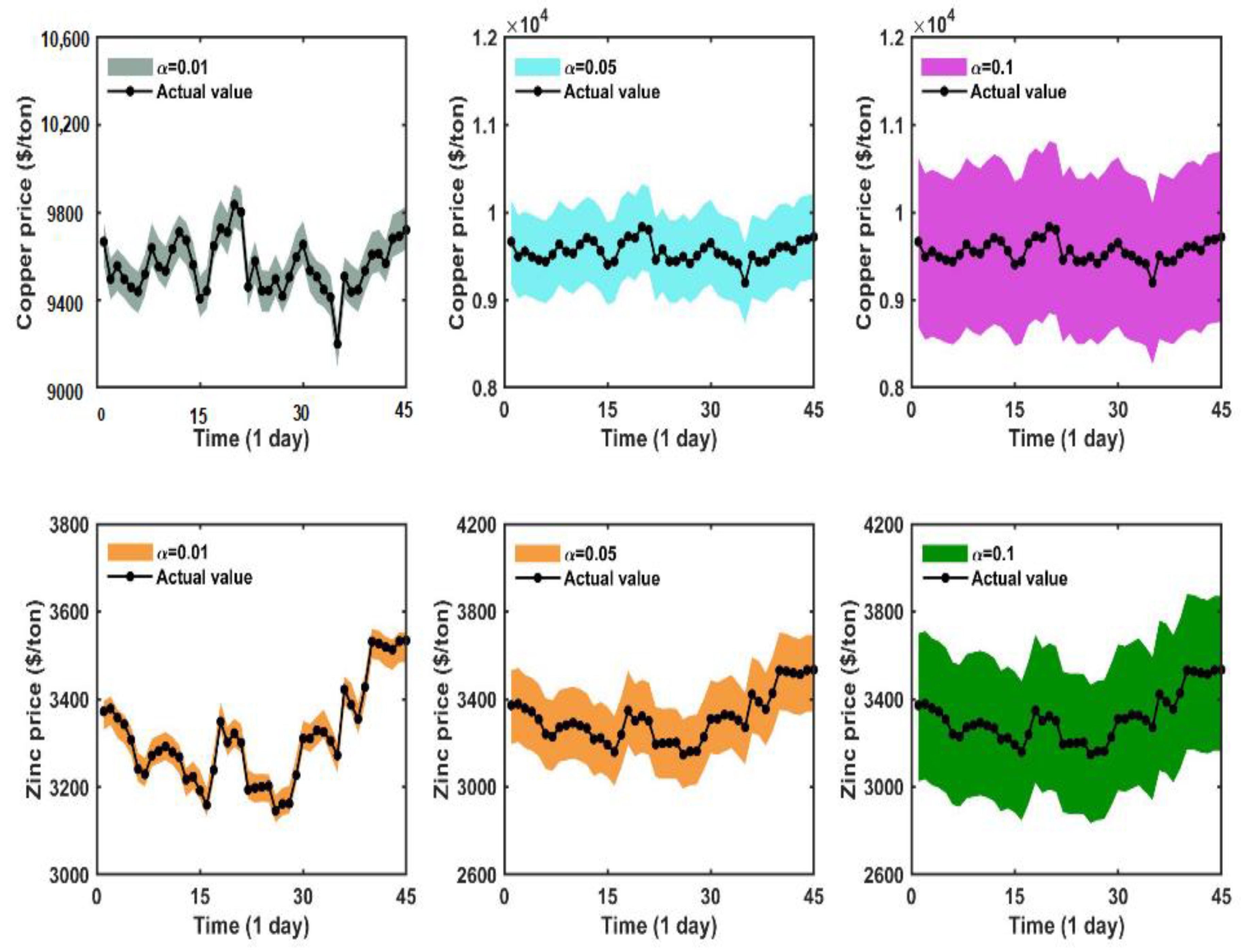
Table 1.
Statistical values of each experimental dataset.
| Dataset | Number | Mean | Std | Min | Max | Kurtosis | Skewness |
|---|---|---|---|---|---|---|---|
| Copper | |||||||
| Training | 720 | 6376.111111 | 913.093217 | 4630.000000 | 9412.500000 | 2.010163 | 1.461172 |
| Validation | 135 | 9601.925926 | 365.311641 | 8894.000000 | 10,460.000000 | −0.409698 | 0.586835 |
| Testing | 45 | 9555.422222 | 122.390023 | 9199.500000 | 9835.000000 | 0.547678 | −0.032925 |
| All Samples | 900 | 7018.948889 | 1529.610952 | 4630.000000 | 10,460.000000 | −0.824881 | 0.825347 |
| Zinc | |||||||
| Training | 720 | 2467.443056 | 271.680217 | 1815.500000 | 3178.000000 | −0.443849 | −0.374203 |
| Validation | 135 | 3031.100000 | 163.270136 | 2814.000000 | 3794.500000 | 6.714848 | 2.434975 |
| Testing | 45 | 3311.277778 | 110.050792 | 3146.000000 | 3534.000000 | −0.245023 | 0.679581 |
| All Samples | 900 | 2594.183333 | 361.556747 | 1815.500000 | 3794.500000 | −0.131702 | 0.190299 |
Table 2.
Performance metric rules.
| Metric | Equation |
|---|---|
| MAE | |
| RMSE | |
| MAPE | |
| IA | |
| TIC | |
| PICP | |
| PINAW | |
| PIAW | |
| Score |
Note: and are the actual and predicted non-ferrous metal price values, respectively, N is the number of data, and , where and are the interval lower and upper bounds, respectively, and is the significance level.
Table 3.
Optimal sub-model for each mode.
| Mode | Copper | Zinc | Yes or No? |
|---|---|---|---|
| Mode No1 | ORELM | ELM | No |
| Mode No2 | WRELM | WRELM | Yes |
| Mode No3 | ORELM | ELM | No |
Note: Yes, means that the best sub-models of datasets copper and zinc are the same; No, means that the best sub-models of datasets copper and zinc are not the same.
Table 4.
Results of two datasets point forecasting.
| Dataset | Model | MAE | RMSE | MAPE(%) | IA | TIC |
|---|---|---|---|---|---|---|
| Copper | ELM | 112.334560 | 135.637098 | 1.172072 | 0.662147 | 0.007129 |
| RELM | 111.333267 | 134.997478 | 1.161670 | 0.665282 | 0.007095 | |
| WRELM | 106.203165 | 130.771381 | 1.108749 | 0.678176 | 0.006869 | |
| ORELM | 110.438731 | 135.872875 | 1.152984 | 0.675115 | 0.007139 | |
| SVMD-ELM-SE | 32.060023 | 35.557911 | 0.334526 | 0.977442 | 0.001864 | |
| SVMD-RELM-SE | 37.106249 | 39.805757 | 0.387352 | 0.971950 | 0.002087 | |
| SVMD-WRELM-SE | 39.118255 | 41.766036 | 0.408252 | 0.968886 | 0.002190 | |
| SVMD-ORELM-SE | 29.982821 | 33.566644 | 0.312725 | 0.979759 | 0.001759 | |
| The Developed System | 11.332665 | 14.359648 | 0.118469 | 0.996536 | 0.000751 | |
| Zinc | ELM | 94.530373 | 108.820780 | 2.814554 | 0.725792 | 0.016660 |
| RELM | 100.782507 | 114.889654 | 3.001630 | 0.702154 | 0.017607 | |
| WRELM | 96.771240 | 111.029926 | 2.881543 | 0.717259 | 0.017004 | |
| ORELM | 111.434073 | 126.324646 | 3.318488 | 0.653617 | 0.019392 | |
| SVMD-ELM-SE | 35.986381 | 40.118159 | 1.072213 | 0.961745 | 0.006088 | |
| SVMD-RELM-SE | 37.135380 | 41.369084 | 1.106171 | 0.959088 | 0.006279 | |
| SVMD-WRELM-SE | 57.910982 | 62.859317 | 1.728839 | 0.906204 | 0.009571 | |
| SVMD-ORELM-SE | 44.020481 | 48.100182 | 1.313996 | 0.945457 | 0.007308 | |
| The Developed System | 6.757693 | 8.351136 | 0.203406 | 0.998478 | 0.001260 |
Table 5.
Point forecasting results of two datasets based on the model selection strategy.
| Dataset | Model | MAE | RMSE | MAPE(%) | IA | TIC |
|---|---|---|---|---|---|---|
| Copper | SVMD-OMSELM-SE | 29.794091 | 33.391426 | 0.310760 | 0.979977 | 0.001750 |
| SVMD-OMSELM-NE1 | 11.523120 | 14.584133 | 0.120518 | 0.996438 | 0.000763 | |
| SVMD-OMSELM-NE2 | 11.921647 | 15.262713 | 0.124665 | 0.996111 | 0.000798 | |
| SVMD-OMSELM-NE3 | 11.903481 | 15.065372 | 0.124446 | 0.996195 | 0.000788 | |
| The Developed System | 11.332665 | 14.359648 | 0.118469 | 0.996536 | 0.000751 | |
| Zinc | SVMD-OMSELM-SE | 35.945599 | 40.060919 | 1.071027 | 0.961865 | 0.006079 |
| SVMD-OMSELM-NE1 | 7.822494 | 9.649678 | 0.236055 | 0.997973 | 0.001455 | |
| SVMD-OMSELM-NE2 | 8.166177 | 10.071516 | 0.247068 | 0.997776 | 0.001519 | |
| SVMD-OMSELM-NE3 | 7.881242 | 9.427713 | 0.237614 | 0.998025 | 0.001422 | |
| The Developed System | 6.757693 | 8.351136 | 0.203406 | 0.998478 | 0.001260 |
Table 6.
Interval prediction results for Copper and Zinc price.
| Dataset | Alpha | PICP | PIAW | PINAW | SCORE |
|---|---|---|---|---|---|
| Copper | 0.010000 | 100.000000 | 190.713983 | 0.300101 | −3.814280 |
| 0.050000 | 100.000000 | 955.486526 | 1.503519 | −95.548653 | |
| 0.100000 | 100.000000 | 1912.229981 | 3.009016 | −573.668994 | |
| Zinc | 0.010000 | 100.000000 | 65.090031 | 0.167758 | −1.301801 |
| 0.050000 | 100.000000 | 331.094291 | 0.853336 | −33.109429 | |
| 0.100000 | 100.000000 | 663.347551 | 1.709659 | −132.66951 |
Disclaimer/Publisher’s Note: The statements, opinions and data contained in all publications are solely those of the individual author(s) and contributor(s) and not of MDPI and/or the editor(s). MDPI and/or the editor(s) disclaim responsibility for any injury to people or property resulting from any ideas, methods, instructions or products referred to in the content. |
© 2023 by the authors. Licensee MDPI, Basel, Switzerland. This article is an open access article distributed under the terms and conditions of the Creative Commons Attribution (CC BY) license (https://creativecommons.org/licenses/by/4.0/).
Share and Cite
MDPI and ACS Style
Yang, S.; Yang, W.; Zhang, K.; Hao, Y. A Novel System Based on Selection Strategy and Ensemble Mode for Non-Ferrous Metal Futures Market Management. Systems 2023, 11, 55. https://doi.org/10.3390/systems11020055
AMA Style
Yang S, Yang W, Zhang K, Hao Y. A Novel System Based on Selection Strategy and Ensemble Mode for Non-Ferrous Metal Futures Market Management. Systems. 2023; 11(2):55. https://doi.org/10.3390/systems11020055
Chicago/Turabian StyleYang, Sibo, Wendong Yang, Kai Zhang, and Yan Hao. 2023. "A Novel System Based on Selection Strategy and Ensemble Mode for Non-Ferrous Metal Futures Market Management" Systems 11, no. 2: 55. https://doi.org/10.3390/systems11020055
Note that from the first issue of 2016, this journal uses article numbers instead of page numbers. See further details here.