Abstract
The quantitative evaluation of the coupling coordination degree (CCD) between the regional economy and eco-environment systems is of great importance for the realization of sustainable development goals, which could identify economic or eco-environmental cold areas. To date, traditional evaluation frameworks mainly include the indicator system construction based on statistical data, which seldom utilize the geo-spatiotemporal datasets. Hence, this study aimed to evaluate the CCD change trend of the Yangtze River Delta (YRD) and explore the relationship between the CCD, economy, and eco-environment on the county scale. In this study, YRD was selected as the study area to evaluate its level of CCD at different periods, and then the nighttime difference index (NTDI) and eco-environmental comprehensive evaluation index (ECEI) were calculated to represent the difference in the development of the regional economy and the eco-environmental quality (EEQ). The CCD between the two systems was then calculated and analyzed using global, local, and Geary’s C spatial autocorrelation indicators, in addition to change trend methods. The main findings showed that: (1) During the period 2000–2020, the economic system in YRD showed a continuously upward trend (0.0487 a−1), with average NTDI values of 0.2308, 0.2964, 0.3223, 0.3971, and 0.4239, respectively. In spatial terms, the economy system showed a distribution of “high in the east and low in the west”. (2) YRD’s EEQ indicated a gradual upward trend (from 0.3590 in 2000 to 0.3970 in 2020), with a change trend value of 0.0020 a−1. Spatially, the regions with high ECEI were mainly located in southwestern counties. (3) In the past 20 years, the CCD between economic and eco-environment systems showed an increased change trend, with a change trend value of 0.0302 a−1. The average CCD values for the five periods were 0.3992, 0.4745, 0.4633, 0.5012, and 0.5369. The overall level of CCD improved from “moderate incoordination” to “low coordination”. (4) Both NTDI and ECEI indexes have a positive effect on the improvement of regional CCD. However, the contribution of NTDI is a little higher than that of ECEI.
1. Introduction
With the implementation of the reform and opening policy in 1978, the level of urbanization in China has continuously improved [1]. According to the China Statistical Yearbook (2022) issued by the National Bureau of Statistics, the urbanization rate increased from 17.92% in 1978 to 64.72% in 2021 [2]. Furthermore, according to the United Nations report, the percentage of the population residing in urban areas is expected to reach 68.4% by 2050 [3]. However, accompanied by the rapid development of urbanization in China, a series of eco-environmental issues have emerged, such as water and soil loss [4,5], biodiversity reduction [6], the decrease in forest cover rate [7], the frequent occurrence of high-temperature disasters [8,9], and loss of wetland [10]. In this context, the Chinese government implemented the regional coordinated development strategy in 2017, which aims to narrow the gap between different regions and achieve harmonious development between the eco-environment and economic systems in each region [11]. Of these regions, the Yangtze River Delta (YRD) is one of the most important regions for promoting the development of the country’s economy, as it has always been considered a leader and an engine of economic development [12]. Therefore, it is of great significance to assess the trends and characteristics of the spatiotemporal evolution of the YRD.
To date, numerous scholars have conducted studies on the evaluation of the economy, urbanization, and eco-environment systems and the coupling coordination degree analysis between these systems. To be specific, Ji et al. investigated the trend of change in the degree of coordinated development between six elements, which were population, society, economy, resources, ecology, and the environment. Based on statistical data and remote sensing data, the evaluation index system for each element was established. Meanwhile, the coordinated index and the coordinated development index were promoted to assess the level of coordinated development. In his research, standard deviation value and average value were applied to evaluate the development gap between different cities [13]; Weng et al. established the subsystem of economy, the environment, and society to evaluate the coupling relationships between them. Among them, the economy subsystem included three indicators, which were GDP per capita, the proportion of the tertiary industry added to the local GDP, and the registered urban unemployment rate. In their study, the 31 Chinese provinces were taken into consideration to evaluate their pattern of change [14]. Dong et al. constructed an index system to evaluate the coordinated level of the regional economy, technology, and renewable energy systems. Specifically, the economy subsystem included GDP, GDP per capita, the total import and export of goods, the urbanization rate, the proportion of tertiary industry output in GDP, and the registered urban unemployment rate [15]. Han et al. measured the coupling coordinated state between the digital economy, technological innovation, and eco-environment systems. Specifically, the eco-environment subsystem included nine indicators from three aspects, which were pressure, endowment, and governance results [16]. Chu et al. also chose the aspects of population, economy, society, and eco-environment to evaluate their degree of coupling coordination in Russia. In their investigation, the economy subsystem selected seven indicators. In addition, they found that the overall situation of the level of urbanization in Russia still belonged to the moderate uncoordinated recession stage [17].
In summary, existing studies mainly used statistical data to calculate each subsystem level by selecting several indicators. Research datasets, used in these studies, were primarily derived from the regional statistical yearbook. However, although statistical data have the advantage of high authority, they also have obvious disadvantages, such as incomplete statistical indicators, inconsistent statistical calibers, and an inability to provide spatial information [18]. Furthermore, statistical data has such problem, existing indicators cannot meet study requirements, while the required indicators cannot be calculated. Compared with statistical data, geospatial data, especially remote sensing data, provide a useful tool for the evaluation of the regional economy and the eco-environment [19]. To be specific, Ye et al. applied nighttime light data to analyze the spatiotemporal characteristics of urbanization in the Taiwan Strait; they found that nighttime light data increased from 729, 863 in 1992 to 2, 729, 0552 in 2020, with the percentage of high-value light changing from 2.59% to 12.22% [20]. Liu et al. also utilized nighttime light data to evaluate the characteristic of change before and after COVID-19 in mainland China [21]. Generally, nighttime light from different regions is positively correlated with the level of regional economy [22,23,24], and the total amount of nighttime light can be used to reflect the level of regional economic development. Furthermore, some scholars established the comprehensive nighttime light index (CNLI) to reflect regional urbanization or the level of the economy [25,26,27]. For example, Luo et al. took central Shanghai as the study area to investigate the degree of coupling coordination between urbanization and the eco-environment [25]. Tang et al. constructed an improved CNLI by integrating the principal component analysis (PCA) method to evaluate the degree of local- and telecoupling coordination between urbanization and the eco-environment. Their results found that the Wuhan urban group improved from an uncoordinated state to a coordinated state [28]. Generally, most studies used night light to reflect the overall economy or urbanization level; however, night light data could not reflect the per capita occupancy [18]. With the advent of the big data era, numerous studies have published many datasets, including land use/land cover data with fine resolution [29,30], population density data [31,32,33,34,35], etc. Among them, WorldPop data estimated the amount and density of the global population at 100 m resolution after adjustment, which had been widely used [18,36,37,38]. Therefore, it could calculate the nighttime difference index (NTDI) to reflect the regional economic development equality by combining WorldPop data with NPP-VIIRS-like nighttime light data.
The eco-environment is defined as “the total quantity and quality of water resources, land resources, biological resources, and climate resources that affect human survival and development” [18,39]. It belonged to a social-economic-natural compound system [39]. To date, the evaluation of regional eco-environmental quality has attracted the widespread attention of scholars at home and abroad. For instance, Bai et al. selected eight indexes, including precipitation, temperature, net primary productivity, normalized difference vegetation index (NDVI), digital elevation model, land use and land cover (LULC), population, and potential evapotranspiration to calculate the comprehensive EEQ of China, integrating the entropy method. They found that the EEQ of more than 60% of the area increased from 2000 to 2017 [40]. Yang et al. applied the remote sensing ecological index (RSEI) and the MODIS product to evaluate the EEQ of the Yangtze River Basin from 2001 to 2019, concluding that the average RSEI showed an overall upward trend with a growth rate of 0.027 year−1 [41]. Li et al. promoted a modified remote sensing ecological index named remote sensing ecological environment index (RSEEI) by integrating NDVI, land surface temperature (LST), wetness (WET), normalized difference build-up and soil index (NDBSI), biological abundance, and environmental pollution index. This index was applied to assess the EEQ of China; its results indicated that the change rate of the EEQ was −0.00011 a−1, indicating that the EEQ in China showed a downward trend in the past 20 years [42]. Generally, evaluating the regional EEQ consisted mainly of two aspects, which were indicators’ selection and accurate assessment. Regarding the selection of indicators, existing studies could be divided into single indicators, such as NDVI, and integrations of multiple indicators, such as RSEI, comprehensive evaluation index (CEI) [43], ecological environmental index (EEI) [44], etc. Among them, RSEI was promoted by Xu [45], considering greenness, wetness, heat, and dryness, which had been widely applied [18,41,46]. However, in practical applications, it was found that RSEI also had some limitations, including the failure to consider season difference, the effect of water bodies, the LULC difference, etc. In response to solving or improving these problems, Xu et al. introduced LULC and RSEI to establish RSEI-2 to evaluate the China EEQ, they found that RSEI-2 had a high precision compared to RSEI in evaluating the regional EEQ [26]. Zhang et al. took the season difference into account to evaluate Tianjin’s EEQ, and they concluded that the annual average RSEI of four seasons would be more appropriate to characterize the trend of change in the EEQ [47]. However, Xu and Deng thought that it was inappropriate to give these indexes RSEI-related names when adding non-ecological indicators [48]. In this context, Ji et al. both considered the differences in LULC and season, and promoted an eco-environmental comprehensive evaluation index (ECEI), their results found that ECEI had good stability and precision [19]. On this basis, the ECEI calculation method could be applied to calculate the EEQ of YRD.
To date, the relationship between the economy or urbanization and the eco-environment has been studied. Sarkodie and Strezov promoted the environmental Kuznets curve hypothesis (EKC) [49]. Except for the EKC hypothesis, other theories have also been promoted. For instance, the urban metabolism theory [50], footprint family theory [51], tele-coupling theory [52], planetary boundaries theory [53], coupling coordination degree model (CCDM) [54], stochastic impacts by regression on population, affluence and technology model [55], and multi-agent model [56]. In particular, the EKC and CCDM models were widely used. Among them, the EKC hypothesis showed that there existed an inverted “U” shape between the economy and the eco-environment. However, this hypothesis was not fully supported in developing regions. Moreover, the EKC hypothesis failed to evaluate the interaction between the economy and eco-environment systems. Compared with the EKC hypothesis, CCDM was one model that could evaluate the coupling coordination degree between two or more subsystems. Specifically, the concept of coupling originates from physics; it refers to a phenomenon which two or more subsystems affect each other via miscellaneous interactions [54]. To date, CCDM has been widely applied in investigating the coupling coordinated level between the economy, society, eco-environment, or other subsystems [57,58,59]. However, CCDM failed to distinguish cases with different degrees of coupling and comprehensive development levels, but with the same degree of coupling coordination [18].
Based on the aforementioned content, this paper aimed to explore the spatiotemporal change trend of CCD between eco-environmental and economic systems over the past 20 years. Given existing shortcomings, this study introduced the NTDI to represent the quality of economic development rather than the simple economy level, applied the ECEI to evaluate the regional EEQ, and modified the CCDM to evaluate the CCD between the two systems. This paper is organized as follows: the Material and Methods section presents the study area, data sources and methods, which include the calculation of NTDI, ECEI, and CCD, meaning the global and local spatial autocorrelation index and the change trend method, respectively; the Results section describes the spatiotemporal distribution situation of the NTDI, ECEI, and CCD; the Discussion section presents the validation and comparison results of ECEI and RSEI, analyzes the global, local and Geary’s C spatial autocorrelation calculation results of CCD and its policy implications, explores the relationship between NTDI, ECEI, and CCD, and provides the limitations and ideas for further study; and the Conclusion section presents the key findings of this paper.
2. Materials and Methods
2.1. Study Area
YRD is located in the eastern coastal area of China, with a latitude and longitude range of 115°46′∼123°25′ E, 29°20′∼32°34′ N. The YRD covers an area of 211.7 thousand square kilometers (Figure 1). YRD includes 27 cities at the prefecture level. Specifically, Shanghai is a municipality directly under the central government, Chizhou, Tongling, Wuhu, Maanshan, Anqing, Xuancheng, Hefei, and Chuzhou belong to Anhui province; Yancheng, Yangzhou, Zhenjiang, Taizhou, Nantong, Nanjing, Changzhou, Wuxi, and Suzhou belong to Jiangsu province; and Huzhou, Jiaxing, Zhoushan, Hangzhou, Shaoxing, Ningbo, Jinhua, Taaizhou, and Wenzhou belong to Zhejiang province. YRD is one of the most developed regions in all of China, and is one of its important economic growth engines, with the other two being Jing-Jin-Ji and Pearl River Delta. According to the China Statistical Yearbook (2022) [2], the total permanent resident population and gross domestic product (GDP) in 2021 reached approximately 0.236 billion people and 27.6 trillion yuan, representing 16.7% and 24.1% of the whole of China, respectively. Additionally, the population urbanization rate reaches 70%. However, with the acceleration of urbanization process, a large number of people living in rural areas flowed into urban areas, which brought huge pressure on the urban eco-environment. For example, Shanghai had a permanent resident population of 24.894 million people in the year 2021; however, the average annual daily PM10 was 43 μg/m3, which had increased by 4.90% compared to the same period of the previous year. Furthermore, in 2021, Shanghai transported approximately 9.3157 million tons of domestic waste, and this domestic waste puts great pressure on human life quality. In this context, it is of great urgency to quantitatively evaluate the CCD between economic and eco-environmental systems, which will not only reveal the interaction status between the two systems on a small scale, but also provide some solid references for relevant policymakers to better realize regional sustainable development goals.
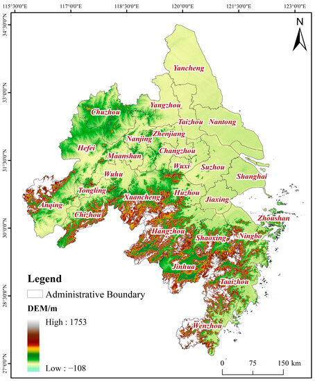
Figure 1.
Location of the study area.
2.2. Data Sources
In this study, the remote sensing datasets and administrative boundary data were collected to evaluate CCD between economic and eco-environment systems. Table 1 shows a brief introduction to each dataset.

Table 1.
A brief introduction to datasets.
According to Table 1, the MOD09A1 product provides the surface spectral reflectance of Terra MODIS bands 1–7 with a resolution of 500 m. For example, seven bands are blue (459–479 nm), green (545–565 nm), red (620–670 nm), nir (841–876 nm), mir1 (1230–1250 nm), mir2 (1628–1652 nm), and mir3 (2105–2155 nm). In addition, seven bands have undergone atmospheric correction. The MOD11A2 product provides the 8-day average LST with a resolution of 1000 m [11,39]. To reduce the cloud pollution problem, the Google Earth Engine (GEE) platform and median method were utilized to acquire the cloud-free images of four seasons in the years 2000, 2005, 2010, 2015, and 2020. Among them, the period for each season was as follows: 1 March to 31 May (Spring), 1 June to 31 August (Summer), 1 September to 30 November (Autumn), and 1 December to 28 February (Winter) [60]. NPP-VIIRS-like nighttime light data were downloaded from Chen’s study [61], and these nighttime light data have fine spatial resolution and good consistency. In addition, the data underwent a new cross-sensor calibration method. WorldPop data were acquired from the WorldPop website; they provide population density spatial data with two types, which were 100 m and 1000 m. Both spatial population density datasets have undergone population calibration using statistical data. In this study, population density data with 100 m resolution for five target years were downloaded. The GLC-FSC30 datasets were evaluated from the Data Sharing and Service Portal website with 30 m resolution. Administrative boundary data provided the boundary of YRD in shapefile format, which was downloaded from the National Geomatics Center of China website. After all datasets were acquired in raster format, they were resampled to 500 m resolution and reprojected to UTM_WGS_1984_50N using the ArcGIS 10.8 version. To be specific, for discrete data (including GLC_FCS30), the nearest neighbor resampling method was used; for continuous datasets (including MOD11A2, NPP-VIIRS-like nighttime light data, and WorldPop data), the bilinear interpolation resampling method was used.
2.3. Methods
Figure 2 shows the framework of this study, which includes four main parts: (1) calculation of NTDI and its spatiotemporal analysis; (2) calculation of ECEI and its spatiotemporal analysis; (3) calculation of CCD and its spatiotemporal analysis; and (4) calculation of global, local, and Geary’s C spatial autocorrelation, and change trend of CCD. Section 2.3.1, Section 2.3.2, Section 2.3.3, Section 2.3.4 and Section 2.3.5 introduce the calculation formulas in detail.

Figure 2.
Framework of this study.
2.3.1. Calculation of NTDI
The Gini coefficient is one indicator used to evaluate the regional income equality, and has been widely used [62]. The value of Gini coefficient ranges from 0 to 1; a larger value indicates a less equal distribution of regional economy. Based on the Gini coefficient, WorldPop data were used to represent the spatial distribution of the regional population, and NPP/VIIRS-like nighttime light data were used to characterize the spatial distribution of the regional economy development level. Therefore, in light of the Gini coefficient, the NTDI index was calculated using the following formula (Equation (1)). Among them, to reduce the impact of outliers, the values of the first 0.1% and the last 0.1% in the histogram were removed.
where nti and ntj indicate the value of nighttime light per capita for regions i and j. represents the mean value of the value of nighttime light per capita for k regions. Among them, the per capita nighttime light value was the quotient of light value and the population density value at each pixel. Similar to the Gini coefficient, the value of NTDI also ranges from 0 to 1; however, for NTDI, the higher the value, the higher the equality. The values of 1 and 0 represent absolute equality and absolute inequality, respectively.
2.3.2. Calculation of ECEI
The ECEI includes five indexes, which are NDVI, WET, NDBSI, LST, and AI. After processing the original MODIS and LULC products, the original ECEI of four seasons was acquired by applying the PCA method. Then, the average ECEI for each period was calculated. Among them, the outliers removal method was the same as for the calculation of NTDI. Equations (2)–(9) were the calculation formulas [63,64].
where rblue, rgreen, rred, rnir, rmir1, rmir2, and rmir3 indicate the surface reflectance of the blue, green, red, nir, mir1, mir2, and mir2, respectively; WET is the moisture calculation formula, one component of the tasseled cap transformation; μ is the normalized coefficient; forest, grassland, water, cropland, built, and unused are the corresponding areas of each land use type in each period; Nrescale represents the normalized result of each index; Ni, Nmin, and Nmax represent the ith, min, and max values of each index, respectively; PCA1 represents the first component of PCA; ECEIseason_t is the origin ECEIseason value; ECEIseason_t_i, ECEIseason_t_min, and ECEIseason_t_max are the ith, min, and max values of ECEIseason_t, respectively; ECEIseason represents the normalized value of ECEIseason_t; ECEI indicates the average value of the four seasons in each period. The ECEI ranges from 0 to 1, and a higher value represents a higher EEQ; in contrast, a smaller value indicates a lower EEQ.
2.3.3. Calculation of CCD
Given that the existing CCD calculation method cannot distinguish between cases with different coupling degrees and comprehensive development levels but the same CCD, from the distance perspective, the coupling value and comprehensive development value were set as the x-axis and y-axis, the distance from the origin point to the line segment was the original CCD, and then the final CCD was calculated by normalizing the original CCD. Equations (10)–(12) show the calculation formulas.
where C is the degree of coupling of the economy and eco-environment systems (in this study, it represents the degree of coupling of NTDI and ECEI); T is the comprehensive development level of the two systems; m and n are the weight value of the two systems (in this study, m and n were set as 0.5 due to the fact that the two systems have the same importance); CCD indicates the value of the modified coupling coordination index, the value of CCD ranges from 0 to 1, and the larger the value, the higher the CCD between NTDI and ECEI. In contrast, the lower the value, the smaller the CCD between NTDI and ECEI. Based on an existing study [28], CCD was divided equally into five grades; the classification criteria for each grade are displayed in Table 2.
Table 2.
Different CCD grade classification criteria.
2.3.4. Calculation of Spatial Autocorrelation Indicators
Spatial autocorrelation describes the correlation between a variable at a specific position and its neighboring position. Spatial autocorrelation includes three types, which are positive, negative, and random distribution. To be specific, the positive distribution indicates that an observed spatial value and its surrounding values have the same direction of change. By contrast, negative distribution represents that one observed spatial value and its surrounding values have the inverse change direction. The random distribution shows that one observed spatial value has no relationship with its surrounding values. Spatial autocorrelation can be measured using global and local indexes. In addition to these two indexes, Chen promoted a new approach to calculating Moran’s I index [65]. Of these indexes, Geary’s C could be an effective index to measure the spatial autocorrelation state. In particular, for small spatial datasets, combining Moran’s I and Geary’s C indexes can provide more convincing results. Equations (13)–(15) show the calculation formulas.
where xi and xj indicate the values in i and j; μ is the average value; wij represents the spatial weight function; N represents the number of pairs of samples. IGlobal is the global spatial autocorrelation value; it ranges from −1 to 1. If it equals 0, it represents that spatial autocorrelation does not exist; if it is greater than 0, it indicates there exists a positive spatial autocorrelation; if it is smaller than 0, it indicates there exists a negative spatial autocorrelation. ILocal is the local spatial autocorrelation value, which calculates each county. Based on the results, it could be divided into four types, which are “High-High Cluster”, “High-Low Outlier”, “Low-High Outlier”, and “Low-Low Cluster”. IGeary is Geary’s C index value; Z is the standardized vector; and s represents the standard deviation. Among them, the value of IGeary ranges from 0 to 2. If it equals 1, spatial autocorrelation does not exist; if it is greater than 1, it indicates there exists a negative spatial autocorrelation; if it is smaller than 1, it indicates there exists a positive spatial autocorrelation.
2.3.5. Calculation of Change Trend Analysis
The change trend analysis method was adopted to assess the change trend of CCD. The principle of change trend analysis is to characterize the change direction and intensity of a variable by using univariate linear regression analysis. The slope of the regression equation indicates the variable’s change trend. The change trend analysis has the several advantages, including simple calculation and low requirements of the sample number [66]. Equation (16) is the calculation formula of the change trend analysis method:
where θslope represents the change; n represents the number of study periods. In this study, n equals 5; Ni is the ith value of NTDI, ECEI, and CCD. If the value of θslope is greater than 0, it shows that the variable represents an increasing change trend; if the value is less than 0, it represents that the variable shows a decreasing change trend.
3. Results
3.1. Spatiotemporal Analysis of NTDI
Based on the NTDI calculation results, the average NTDI values of five periods were calculated. The mean NTDI values were 0.2308, 0.2964, 0.3223, 0.3971, and 0.4239, respectively. Generally, the NTDI showed a continuously increasing change trend, with a change trend value of 0.0487. Based on the average NTDI of the city, in 2000, Chizhou city, Xuancheng city, and Chuzhou city had a low value of NTDI, with a value lower than 0.10, indicating that the equality of economic development of these cities was low. However, the NTDI of the Shanghai municipality had the highest value (0.4873). In 2005, Chizhou city still had the lowest NTDI value (0.0485), while Shanghai municipality had the highest value (0.5485). In 2010, the NTDI values of Chizhou city and Shanghai municipality were 0.0717 and 0.5527, respectively. In the years 2015 and 2020, the NTDI values of Chizhou city were 0.0938 and 0.1078, while the values of Shanghai municipality were 0.5774 and 0.5803. Furthermore, in 2000, the NTDI values of 15 cities were lower than the average value of this period, while the NTDI values of 12 cities were higher than the average values of this period. In 2005, the NTDI values of 15 cities were lower than the average value of this period, while the NTDI values of 12 cities were higher than the average value of this period. Among them, the NTDI of Zhenjiang city increased by 60.44%, with the NTDI value increasing from 0.1805 to 0.2896. In 2010, 14 cities’ NTDI values were lower than the average value of this period, while 13 cities’ NTDI values were higher than the average value of this period. Compared with 2005, in 2010, Yangzhou city had changed from an under-average value state to an above-average state, indicating that the difference in economic development had decreased. In 2015, the NTDI values of eleven cities were lower than the average value of this period, while the NTDI values of fourteen cities were higher than the average value of this period. Unlike the period of 2010, the NTDI values of Huzhou city and Jinhua city had changed from a below-average value state to the above-average state. In 2020, the NTDI values of 12 cities were lower than the average value of this period, while the NTDI values of 13 cities were higher than the average value of this period. In this period, Zhoushan city had changed from an above-average value state to a below-average state. Zhoushan city was made up of several islands, and the regions with a high economic development level were located mainly in the central districts. Generally, in the past 20 years, Chizhou city, Xuancheng city, Chuzhou city, Anqing city, and Tongling city were the last five cities; these cities all belong to Anhui province, which had low level of economic development. From the perspective of the change trend, the change trend of all cities showed an increased change trend, indicating that the difference in economic development of all cities had narrowed. To be specific, Taaizhou city had the highest change trend, with a value of 0.0835, while Hefei city had the lowest change trend, with a value of 0.0142.
To better understand the characteristics of spatiotemporal distribution at the county level, the average value of the NTDI value of 212 counties was calculated; Figure 3 presents the spatial distribution maps of the five periods. According to Figure 3, in 2000, the NTDI values of 141 counties were lower than the average value of this period, while the NTDI values of 91 counties were higher than the average value of this period. Among them, the Bowang district of Maanshan city had the lowest NTDI value (0.0015), while the Xiacheng district had the highest NTDI value (0.8051). In 2005, the NTDI values of 141 counties were lower than the average value of this period, while the NTDI values of 97 counties were higher than the average value of this period. Compared with 2000, in 2005, the NTDI values of six counties were higher than their corresponding study period; for example, Binhu district and Wuzhong district had changed from a below-average state to an above-average state. In 2010, the NTDI values of 110 counties were lower than the average value of this period, while the NTDI values of 102 counties were higher than the average value of this period. Compared to 2005, in 2010, the NTDI values of five counties were higher than their corresponding study period. Among them, Jiangning district, Changshu county, Shangyu district, Yangzhong county, and Pinghu county had changed from a below-average state to an above-average state. In 2015, the NTDI values of 95 counties were lower than the average value of this period, while the NTDI values of 117 counties were higher than the average value of this period. Compared to 2010, in 2015, 15 counties had changed from a below-average state to an above-average state. For example, the NTDI value of the Jintan district had increased from 0.2686 (2010) to 0.5137 (2015), with its NTDI value increasing by 91.25%, indicating that the economic development difference of the Jintan district had narrowed greatly from 2010 to 2015. In 2020, the NTDI values of 86 counties were lower than the average value of this period, while the NTDI values of 126 counties were higher than the average value of this period. Compared with 2015, in 2020, nine counties had changed from a below-average state into an above-average state. Among them, the NTDI value of the Chongming district had increased from 0.3258 (2015) to 0.4468 (2020). In general, in the last 20 years, the NTDI values of 35 counties have changed from a below-average state to an above-average state. Based on each county’s change trend value, the change trend values of 18 counties in NTDI were negative, while the change trend values of 194 counties in NTDI were positive. Specifically, Dongtou district, Pujiang county, and Jindong district were the top three counties with high change trend values; their NTDI change trend values were 0.1452 a−1, 0.1210 a−1, and 0.1175 a−1.
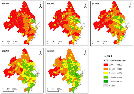
Figure 3.
Spatial distribution maps of NTDI in YRD.
From a spatial perspective, from 2000 to 2020, counties with a high NTDI value had expanded. In 2000, only a few counties in Shanghai municipality belonged to the first echelon. However, in 2020, except for Shanghai municipality, the counties located in southern Jiangsu province and northern Zhejiang province also belonged to the first echelon. In general, in the past 20 years, the NTDI value of the most counties in YRD had increased, indicating that the economic development difference of these regions had gradually narrowed.
3.2. Spatiotemporal Analysis of ECEI
Based on the results of the ECEI calculation, the average ECEI values of five periods were calculated. The mean ECEI values were 0.3590, 0.4174, 0.3715, 0.3610, and 0.3970, respectively. Generally, the ECEI showed an “N” type change trend, with a change trend value of 0.0020 a−1. At the city level, in 2000, the average value of the ECEI of fourteen cities was less than the average value of this period, while the average value of the ECEI of 13 cities was higher than the average value of this period. To be specific, Jiaxing city, Shanghai municipality, and Nantong city were the last three cities, with values of 0.2753, 0.2920, and 0.3110. It could be found that cities with low ECEI values were mainly distributed in Jiangsu province. In 2005, the ECEI values of 16 cities were lower than the average value of this period, while the average value of 11 cities ECEI was higher than the average value of this period. Compared to 2000, in 2005, Chuzhou city and Yangzhou city had changed from an above-average state to a below-average state. In 2010, 14 cities’ ECEI values were lower than the average value of this period, while 13 cities’ ECEI values were higher than the average value of this period. Compared to 2005, in 2010, Wuhu city and Tongling city had changed from the below average state to the above average state. In 2015, the ECEI values of 15 cities were lower than the average value of this period, while the ECEI values of 12 cities were higher than the average value of this period. Compared to 2010, in 2015, Yangzhou city had changed from a below-average state to an above-average state. In 2020, the ECEI values of 16 cities were lower than the average value of this period, while the ECEI values of 11 cities were higher than the average value of this period. Compared to 2015, in 2020, Zhoushan city had changed from the above average state to the below average state. Generally, in the last 20 years, the ECEI values of 12 cities belonged to a below-average state. In particular, the ECEI value of Shanghai municipality is always the lowest one. As an international metropolis, Shanghai is a well-developed city; however, the EEQ of Shanghai municipality is low. From the perspective of change trend, the change trend of nine cities showed a negative value, indicating that the EEQ of these cities had decreased. On the contrary, 18 cities had a positive trend for change. To be specific, Taaizhou city had the lowest change trend, with a value of −0.0028 a−1, while Jiaxing city had the highest change trend, with a value of 0.0127.
To better understand the characteristics of the spatiotemporal distribution at the county level, the average ECEI value of 212 counties was calculated; Figure 4 shows the spatial distribution maps of ECEI in YRD. Figure 5 shows the spatial distribution maps of ECEI at the county level. Based on Figure 4, the overall ECEI during the 2000–2020 period showed a distribution trend of “high in the south and low in the north” and “high in the west and low in the east”. Especially in these southern regions, their ECEI values were high. According to Figure 5, in 2000, the ECEI values of 103 counties were lower than the average value of this period, while the ECEI values of 109 counties were higher than the average value of this period. Among them, Haiyan county of Jiaxing city had the lowest ECEI value (0.2554), while Panan county of Jinhua city had the highest ECEI value (0.4591). In 2005, the ECEI values of 107 counties were lower than the average value of this period, while the ECEI values of 85 counties were higher than the average value of this period. Compared to 2000, in 2005, the ECEI values of 24 counties were lower than their corresponding study period, for example, the Shangcheng district of Hangzhou city and the Xuanwu district of Nanjing city had changed from an above-average state to a below-average state. In 2010, the ECEI values of 141 counties were lower than the average value of this period, while the ECEI values of 98 counties were higher than the average value of this period. Compared to 2005, in 2010, the ECEI values of 13 counties were higher than in their corresponding study period. Among them, Jianhu county of Yancheng city, Baoying county of Yangzhou city, and Wuxing district of Huzhou city had changed from a below-average state into an above-average state. In 2015, the ECEI values of 141 counties were lower than the average value of this period, while the ECEI values of 97 counties were higher than the average value of this period. Compared with 2010, in 2015, one county had changed from an above-average state into a below-average state. The ECEI value of Langxi county of Xuancheng city decreased from 0.3656 (2010) to 0.3467 (2015), with its ECEI value decreasing by 5.17%, indicating that the EEQ of Langxi county had decreased from 2010 to 2015. In 2020, the ECEI values of 113 counties were lower than the average value of this period, while the ECEI value of 99 counties were higher than the average value of this period. Compared to 2015, in 2020, two counties had changed from the below average state into the above average state. Among them, the ECEI values of Haimen district in Nantong city had increased from 0.3252 (2015) to 0.3859 (2020). In general, in the past 20 years, the ECEI values of 10 counties had changed from an above average state to a below-average state. Based on each county’s change trend value, 52 counties’ ECEI change trend values were negative, while 160 counties’ ECEI change trend values were positive. Specifically, Panan county of Jinhua city had the lowest change trend value (−0.0097 a−1), while Haiyan county of Jiaxing city had the highest change trend value (0.0167 a−1).
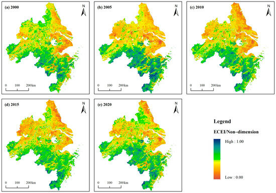
Figure 4.
Spatial distribution maps of ECEI in YRD.
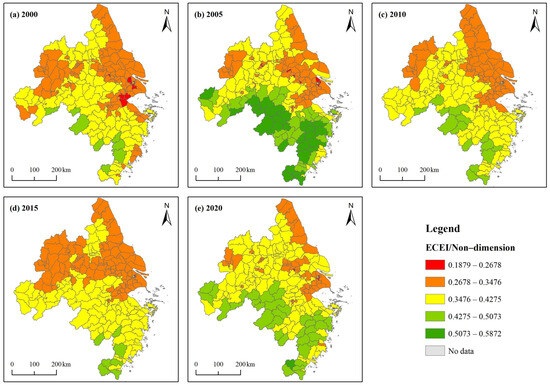
Figure 5.
Spatial distribution maps of ECEI at the county level in YRD.
3.3. Spatiotemporal Analysis of CCD
Based on the results of the CCD calculation, the average CCD values of five periods were calculated. The mean CCD values were 0.3992, 0.4745, 0.4633, 0.5012, and 0.5369, respectively. Generally, the CCD showed an upward change trend, with a change trend value of 0.0302 a−1. At the city level, in 2000, the average value of CCD of fourteen cities was lower than the average value of this period, while the average value of CCD of 13 cities was higher than the average value of this period. To be specific, Chizhou city, Xuancheng city, and Chuzhou city were the last three cities, with values of 0.2824, 0.2930, and 0.2962. It could be found that cities with low CCD values were mainly distributed in Anhui province. In 2005, the CCD values of 14 cities were lower than the average value of this period, while the average value of 13 cities’ CCD values was higher than the average value of this period. Compared to 2000, in 2005, Yangzhou city had changed from an above-average state to a below-average state, while Jinhua city had changed from a below-average state to an above-average state. In 2010, 14 cities’ CCD values were lower than the average value of this period, while 13 cities’ CCD values were higher than the average value of this period. Compared to 2005, in 2010, Jiaxing city and Zhenjiang city had changed from a below-average state to an above-average state, while Huzhou city and Zhoushan city had changed from an above-average state to a below-average state. In 2015, the CCD values of 11 cities were lower than the average value of this period, while the ECEI values of 16 cities were higher than the average value of this period. Compared to 2010, in 2015, Taizhou city, Huzhou city, and Zhoushan city had changed from a below-average state to an above-average state. In 2020, the CCD values of 12 cities were lower than the average value of this period, while the CCD values of 15 cities were higher than the average value of this period. Compared to 2015, in 2020, Zhoushan city had changed from an above-average state to a below-average state. Generally, in the last 20 years, the CCD values of ten cities always belonged to a below-average state. In particular, the CCD value of Chizhou city is always the lowest one. From the perspective of the change trend, the change trend of all cities showed a positive value, indicating that the CCD of all cities had increased. To be specific, Zhoushan city had the lowest change trend, with a value of 0.0073 a−1, while Jiaxing city had the highest change trend, with a value of 0.0568 a−1.
To better understand the characteristics of the spatiotemporal distribution at the county level, the average CCD value of 212 counties was calculated; Figure 6 shows the spatial distribution maps of CCD in YRD. According to Table 2, the CCD was divided into five grades. According to Figure 6, the spatial distribution trend of the CCD between economy and eco-environment in YRD was “high in the east and low in the west”. Specifically, in 2000, two counties (Bowang district and Wuwei county) belonged to the “serious incoordination” grade, one hundred and twenty-seven counties belonged to the “moderate incoordination” grade, and five counties were in the “moderate coordination” grade. In 2005, the CCD values of all counties were greater than 0.2, indicating that no counties in this period were of the “serious incoordination” grade. At the same time, the number of counties with a grade of “moderate incoordination” had decreased from 127 to 69, with a decrease rate of 45.67%. In this period, the Putuo district of the Shanghai municipality had the highest CCD, with a value of 0.6904 (“moderate coordination” grade). In 2010, Zongyang county of Tongling city had the lowest CCD value (0.2257). Compared to 2005, in 2010, the CCD grade of two counties had changed from the “moderate incoordination” grade to the “low coordination” grade. Furthermore, eight counties were in the “moderate coordination” grade. In 2015, Zongyang county of Tongling city still had the lowest CCD value (0.2359), while Longgang county of Wenzhou city had the highest CCD value (0.6565). During this period, 48 counties were in the “moderate incoordination” grade. Compared to 2010, in 2015, the CCD grade of 19 counties had changed from the “moderate incoordination” grade to the “low coordination” grade. On the contrary, the number of counties of grade “moderate coordination” had increased from 8 to 22. In 2020, Mingguang county of Chuzhou city had the lowest CCD value (0.2823), while Yurao county of Ningbo city had the highest CCD value (0.6563). During this period, 23 counties were in the “moderate incoordination” grade, while 30 counties were in the “moderate coordination” grade. During the 2000–2020 period, the CCD values of 104 counties had improved, with the grade changing from “moderate incoordination” grade to “low coordination” grade. Based on the CCD change trend value, the CCD change trend values of 16 counties were negative, while the CCD change trend values of 206 counties were positive, with the lowest and highest change trend values of −0.0289 a−1 and 0.0856 a−1, respectively.
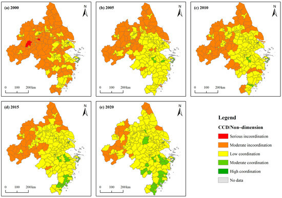
Figure 6.
Spatial distribution maps of CCD in YRD.
4. Discussion
4.1. Validation and Comparison of ECEI and RSEI
In order to validate the results for ECEI, the RSEI values of the five periods were calculated. Figure 7 shows the RSEI column chart for each city in YRD. Figure 8 shows the column graph of each city’s ECEI in YRD. Based on Figure 7, each city’s RSEI showed a fluctuating change trend. In addition, the fluctuation amplitude was larger than the ECEI. However, according to Figure 8, ECEI, which considered land surface and season difference, showed good consistency. Moreover, the change trend also displayed a more stable trend. Furthermore, in 2005, the RSEI of each city was not highest. Compared to 2000, in 2020, the RSEI values of several cities were lower, which was not consistent with the existing data.
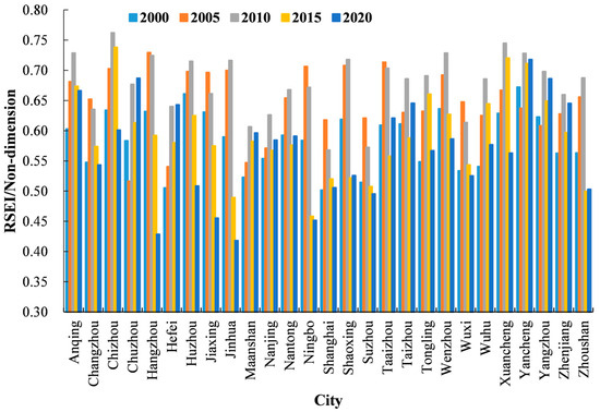
Figure 7.
Column chart of each city’s RSEI in YRD.
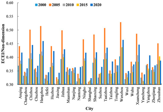
Figure 8.
Column chart of each city’s ECEI in YRD.
Based on statistical data, in the past 20 years, the EEQ of YRD showed an increasing trend of change. Regarding ECEI, most cities displayed the “N” type change. For example, according to the Shanghai Ecological and Environmental Bulletin in 2000 and 2020 [67,68], the average concentration of SO2 in 2000 and 2020 was 22 μg/m3 and 6 μg/m3, respectively, decreased by 72.73%; the average concentration of NO2 in 2000 and 2020 was 56 μg/m3 and 37 μg/m3, which decreased by 33.93%. This indicated that the EEQ of the Shanghai municipality had improved a lot. However, from the RSEI value, during the 2000–2020 period, the RSEI value only increased by 0.78%, while the ECEI value increased by 10.58%, which was close to the actual increase. For example,, Shi et al. considered the air quality aspect and established the modified remote sensing ecological index, and found that the deteriorated regions were mainly concentrated in Shanghai [69]. This conclusion was different from ours. This may be due to the difference between the subfactors. However, combined with the actual result of the EI index, the Shanghai EI value in 2019 was 62.5, indicating that the status of the ecosystem was good, with relatively high vegetation coverage and biodiversity [68]. Therefore, even if there existed a difference between this study and existing studies, when considering the results of the Shanghai Ecological and Environmental Bulletin in different years, it was obvious that the EEQ of Shanghai had improved in the last 20 years.
In addition, the ECEI index of each city was more stable than RSEI. RSEI only considered the various aspects in summer; however, considering four seasons would be more suitable for evaluating regional EEQ. As the regional EEQ was easily influenced by the seasonal difference. Therefore, it would be more appropriate to evaluate regional EEQ considering the difference between seasons.
4.2. Global and Local Spatial Autocorrelation Analysis of CCD and Its Policy Implications
Based on Equation (13), the global Moran’s I value of the five periods was calculated. The values were 0.2662 (2000), 0.1792 (2005), 0.2239 (2010), 0.1883 (2015), and 0.1463 (2020), respectively. The Z-scores of the five periods were all greater than 2.34 and the p-value of the fiver periods was all 0, indicating that the global Moran’s I value passed the significance test at the 0.01 level. Furthermore, the Geary’s C index of the five periods was also calculated; the values were 0.7346 (2000), 0.8527 (2005), 0.7649 (2010), 0.8369 (2015), and 0.8973 (2020), respectively. Similar to global Moran’s I value, the Geary’s C values of the five periods are all smaller than 1, representing that there exists a positive spatial autocorrelation. Based on the global Moran’s I value and Geary’s C value, it could be found that CCD displayed a fluctuating downward trend. This indicated that the degree of spatial autocorrelation had decreased, which meant that the correlation between CCD and spatial location decreased. Combined with the spatial distribution map of local Moran’s I (Figure 9), from 2000 to 2020, the “High-High Cluster” type was mainly distributed in southern coastal regions. For example, the counties in Shanghai municipality, Hangzhou city, Suzhou city, and Wenzhou belonged mainly to the “High-High Cluster” type. In the past 20 years, the number of “High-High Cluster” types showed a fluctuating upward trend, indicating that CCD values in several counties increased. In contrast, the number of “Low-Low Cluster” types also showed a fluctuating upward trend. In 2000, five counties belonged to the “Low-Low Cluster”; however, in 2020, nine counties belonged to this type. Based on Figure 9, it could be found that the “Low-Low Cluster” type is mainly located in the western region, such as Anqing city. Combined with the ECEI and NTDI values of Anqing city, this study found that the NTDI of Anqing city was low.
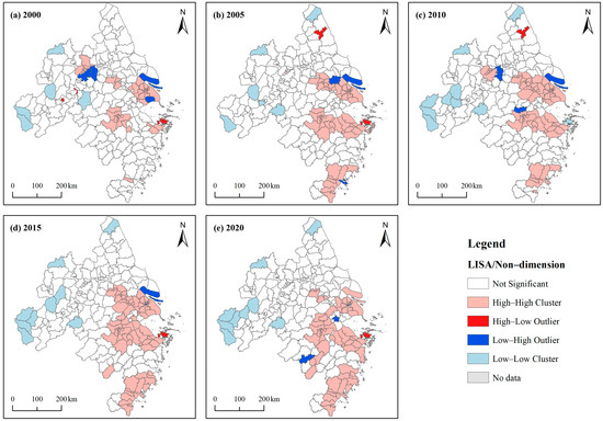
Figure 9.
Local Moran’s I spatial distribution map in YRD.
Based on the aforementioned results, the Shanghai municipality had a high CCD, due to its high NTDI value. Based on the Shanghai Municipal Statistical Yearbooks in 2000 and 2020, the Shanghai GDP indexes were 761.0 and 4290.5, which increased by 463.79%. As an international metropolis, Shanghai’s GDP per capita was 15.58 thousand CNY in 2020, the level of a moderately developed country. Our results were consistent with existing studies. For example, Zhang et al. found that the CNLI of Shanghai municipality and Suzhou city had a high urbanization level [70]. Furthermore, Shao et al. found that the CCD between urbanization and the ecological environment in YRD continuously increased [71]; the CCD value changed from 0.604 (2008) to 0.753 (2017), which further validated our results. In Hu’s study, Shanghai municipality and southern Jiangsu province belonged to the first echelon, with a high level of urbanization [72]. Furthermore, Hu et al. also evaluated the CCD between urbanization and resource environment, and found that the CCD showed a fluctuating upward trend, the value increasing by 2.11% [72]. Xu and Hou constructed one regional urbanization index system, including aspects of population, economy, and land, finding that the YRD economy level showed an upward trend [73], which was consistent with our results. Liu and Wu also found that the comprehensive urbanization level of YRD showed an upward trend [74]. These results demonstrated that the urbanization of the YRD or the level of the economy had improved continuously since the implementation of the reform and opening policy in 1978. Generally, although there existed differences in index selection, data collection, and CCD calculation compared to existing studies, the spatial distribution of economy, eco-environment quality, and CCD was mainly similar to existing studies, which further validated our study.
In order to promote the CCD between economic and eco-environment systems, based on the aforementioned analysis, several suggestions were provided. First, in terms of economy, western cities, such as Chizhou city, Xuancheng city, Chuzhou city, and Anqing city, should focus on improving the level of economic development and narrowing the difference in economic development. However, as for Chuzhou city, Tongling city, Yancheng city, and Maanshan city, both the quality of the eco-environment and the level of economic development need to be further improved. Therefore, more measures must be implemented to narrow the economic development gap. Especially for these cities with low NTDI values, the government should develop more policies to narrow the economic development difference and allow development to benefit more people. Specifically, for these regions with high populations but a poor economy, policy-makers should increase infrastructure investment and upgrade the industry structure. Considering the difference of each region’s development condition, policy-makers should focus on the industry chains with outstanding advantages, and explore and develop characteristic industries in each region. In addition, the residents’ disposable income should increase to promote consumption. Second, from 2000 to 2020, the average ECEI values showed an increasing trend, indicating that the overall EEQ in YRD increased. This was due to the promotion of clean energy and the implementation of regional collaborative governance policies. For instance, YRD has increased eco-environment co-protection and joint governance since 2018. Anhui province has planted about 509.013 thousand hectares of trees. At the same time, the western and southern Anhui provinces were dedicated to constructing the ecological protective screen. In the future, more collaborative projects should be carried out to strengthen the governance of the YRD eco-environment. Finally, in those cities or counties with low CCD values, the government should promote both the NTDI and ECEI values at different amplitudes. For example, Chuzhou city had low values of NTDI, ECEI, and CCD in the last 20 years; in the future, both policies in the aspect of eco-environment governance and improvements of economic development should be put forward to increase the level of interaction. Specifically, local government should promote economic structure transformation by promoting the proportion of tertiary industry, strengthening infrastructure investment, increasing the number of environmentally friendly companies, and implementing the concept of green development.
4.3. Relationship Exploration between NTDI, ECEI, and CCD
To explore the relationship between NTDI, ECEI, and CCD, 1060 county samples from different periods were collected to perform a multiple linear regression analysis. The fitting formula is shown in Table 3.
Table 3.
Fitting formula between NTDI, ECEI, and CCD.
Based on Table 3, the coefficients of ECEI and NTDI were all positive, representing that both indexes could promote the region’s CCD. Specifically, the coefficient of NTDI was a little higher than ECEI. Furthermore, the adjusted R2 was close to 1, at 0.9915, and the significance of the F value was 0.000, which passed the significance test at 0.05 level.
4.4. Limitations and Further Study
This paper explored the spatiotemporal changes of CCD between NTDI and ECEI in YRD. However, this paper still had some limitations. On the one hand, both economy and eco-environment systems belong to complex systems. However, due to the data unavailability, only nighttime light data were collected and used to reflect the economic development difference, which failed to consider the daytime data reflecting economic activities. Owing to the big data era, location-based services’ data and building information data with fine scale provide a new opportunity to evaluate regional daytime economic activity level. These data could be fully utilized to extract valuable information. On the other hand, in this study, the county level was analyzed, and in the future, grid CCD data would be available with the utilization of more new spatial remote sensing datasets.
5. Conclusions
Based on multi-source remote sensing datasets, this study aimed to evaluate the level of economic development and the EEQ of YRD by calculating NTDI and ECEI. Then, the relationship between CCD, NTDI, and ECEI was investigated. The global, local, and Geary’s C spatial autocorrelation analysis methods and the change trend method were then used to analyze the CCD spatial distribution pattern from 2000 to 2020. The main findings of this paper were as follows: (1) During the period of 2000–2020, the economy system in YRD showed a continuously upward trend, showing a distribution of “high in the east and low in the west”. (2) YRD’s EEQ indicated a gradual upward trend, with high ECEI located mainly in southwestern counties. (3) In the past 20 years, the CCD between economy and eco-environment systems showed an increased trend of change, representing a distribution of “high in the eastern coastal regions and low in the northern and western regions”. (4) Both NTDI and ECEI had a positive effect on the improvement of regional CCD. However, the contribution of NTDI was a little higher than ECEI.
Author Contributions
Conceptualization, J.J.; methodology, J.J. and C.Y.; software, J.J., C.Y. and E.S.; validation, L.W. and W.L. (Wenliang Liu); formal analysis, J.J.; investigation, M.X. and W.L. (Wen Lv); resources, J.J. and M.X.; data curation, J.J., M.X., W.L. (Wen Lv) and C.Y.; writing—original draft preparation, J.J.; writing—review and editing, E.S.; visualization, L.W.; supervision, L.W. and W.L. (Wen Lv); project administration, J.J. and W.L. (Wenliang Liu); funding acquisition, J.J. and W.L. (Wenliang Liu). All authors have read and agreed to the published version of the manuscript.
Funding
This research was funded by the Philosophy and Social Science Research in Colleges and Universities of Jiangsu Province (No. 2022SJYB1465), Humanities and Social Sciences Foundation of Suzhou University of Science and Technology (No. XKR202102) and the National Key Research and Development Program of China (No. 2017YFB0503805).
Institutional Review Board Statement
Not applicable.
Informed Consent Statement
Not applicable.
Data Availability Statement
The data presented in this study are available on request from the corresponding author.
Acknowledgments
We thank the National Geomatics Center of China, the United States Geological Survey (USGS), Fuzhou University, and the WorldPop Office for supplying the administrative division data and remote sensing datasets.
Conflicts of Interest
The authors declare no conflict of interest.
Abbreviations
| AI | Abundance index | An index for describing regional biological abundance |
| CCD | Coupling coordination degree | A measure of coupling coordination level between systems |
| CCDM | Coupling coordination degree model | A model of calculating coupling coordination degree |
| ECEI | Eco-environmental comprehensive evaluation index | An index for evaluating regional comprehensive eco-environmental quality |
| EEQ | Eco-environmental quality | A measure of regional eco-environmental quality |
| EI | Ecological index | An index for describing ecological quality |
| GEE | Google earth engine | A cloud platform for processing massive data |
| LST | Land surface temperature | An index for describing regional eco-environmental heat |
| LULC | Land use and land cover | A term of describing land use and land cover |
| NDBSI | Normalized difference build-up and soil index | An index for describing regional eco-environmental dryness |
| NDVI | Normalized difference vegetation index | An index for describing regional eco-environmental greenness |
| NTDI | Nighttime difference index | An index for describing economic development equality |
| RSEI | Remote sensing ecological index | An index for describing eco-environmental quality |
| PCA | Principal component analysis | A method of aggregating multi-dimensional information |
| WET | Wetness | An index for describing regional eco-environmental wetness |
| YRD | Yangtze River Delta | A region in the lower reaches of Yangtze river |
References
- Wen, Q.; Zhang, Z.; Shi, L.; Zhao, X.; Liu, F.; Xu, J.; Yi, L.; Liu, B.; Wang, X.; Zuo, L.; et al. Extraction of basic trends of urban expansion in China over past 40 years from satellite images. Chin. Geogr. Sci. 2016, 26, 129–142. [Google Scholar] [CrossRef]
- National Bureau of Statistics of the People’s Republic of China. China Statistical Yearbook (2022); China Statistics Press: Beijing, China, 2022.
- United Nations, Department of Economic and Social Affairs, Population Division. World Urbanization Prospects: The 2018 Revision; UN: New York, NY, USA, 2021. [Google Scholar]
- Chen, T.; Shu, J.; Han, L.; Tian, G.; Yang, G.; Lv, J. Modeling the effects of topography and slope gradient of an artificially formed slope on runoff, sediment yield, water and soil loss of sandy soil. CATENA 2022, 212, 106060. [Google Scholar] [CrossRef]
- Mohammady, M.; Davudirad, A. Gully Erosion Susceptibility Assessment Using Different Machine Learning Algorithms: A Case Study of Shazand Watershed in Iran. Environ. Model. Assess. 2023, 28, 1–13. [Google Scholar] [CrossRef]
- Daskalova, G.; Myers-Smith, I.; Bjorkman, A.; Blowes, S.; Supp, S.; Magurran, A.; Dornelas, M. Landscape-scale forest loss as a catalyst of population and biodiversity change. Science 2020, 368, 1341–1347. [Google Scholar] [CrossRef] [PubMed]
- Gao, X.; Wang, G.; Innes, J.; Zhao, Y.; Zhang, X.; Zhang, D.; Mi, H. Forest ecological security in China: A quantitative analysis of twenty five years. Glob. Ecol. Conserv. 2021, 32, e01821. [Google Scholar] [CrossRef]
- Verichev, K.; Salazar-Concha, C.; Díaz-López, C.; Carpio, M. The influence of the urban heat island effect on the energy performance of residential buildings in a city with an oceanic climate during the summer period: Case of Valdivia, Chile. Sustain. Cities Soc. 2023, 97, 104766. [Google Scholar] [CrossRef]
- Li, L.; Zhan, W.; Hu, L.; Chakraborty, T.C.; Wang, Z.; Fu, P.; Wang, D.; Liao, W.; Huang, F.; Fu, H.; et al. Divergent urbanization-induced impacts on global surface urban heat island trends since 1980s. Remote Sens. Environ. 2023, 295, 113650. [Google Scholar] [CrossRef]
- Fluet-Chouinard, E.; Stocker, B.; Zhang, Z.; Malhotra, A.; Melton, J.; Poulter, B.; Kaplan, J.; Goldewijk, K.; Siebert, S.; Minayeva, T.; et al. Extensive global wetland loss over the past three centuries. Nature 2023, 614, 281–286. [Google Scholar] [CrossRef]
- Ji, J.; Wang, S.; Zhou, Y.; Liu, W.; Wang, L. Spatiotemporal Change and Landscape Pattern Variation of Eco-Environmental Quality in Jing-Jin-Ji Urban Agglomeration From 2001 to 2015. IEEE Access 2020, 8, 125534–125548. [Google Scholar] [CrossRef]
- Yin, H.; Xiao, R.; Fei, X.; Zhang, Z.; Gao, Z.; Wan, Y.; Tan, W.; Jiang, X.; Cao, W.; Guo, Y. Analyzing “economy-society-environment” sustainability from the perspective of urban spatial structure: A case study of the Yangtze River delta urban agglomeration. Sustain. Cities Soc. 2023, 96, 104691. [Google Scholar] [CrossRef]
- Ji, J.; Wang, S.; Zhou, Y.; Liu, W.; Wang, L. Spatiotemporal Change and Coordinated Development Analysis of “Population-Society-Economy-Resource-Ecology-Environment” in the Jing-Jin-Ji Urban Agglomeration from 2000 to 2015. Sustainability 2021, 13, 4075. [Google Scholar] [CrossRef]
- Weng, Q.; Lian, H.; Qin, Q. Spatial disparities of the coupling coordinated development among the economy, environment and society across China’s regions. Ecol. Indic. 2022, 143, 109364. [Google Scholar] [CrossRef]
- Dong, F.; Xia, M.; Li, W. Evaluation and analysis of regional economic-technology-renewable energy coupling coordinated development: A case study of China. J. Renew. Sustain. Energy 2023, 15, 035902. [Google Scholar] [CrossRef]
- Han, X.; Fu, L.; Lv, C.; Peng, J. Measurement and spatio-temporal heterogeneity analysis of the coupling coordinated development among the digital economy, technological innovation and ecological environment. Ecol. Indic. 2023, 151, 110325. [Google Scholar] [CrossRef]
- Chu, N.; Zhang, P.; Wu, X. Spatiotemporal evolution characteristics of urbanization and its coupling coordination degree in Russia—Perspectives from the population, economy, society, and eco-environment. Environ. Sci. Pollut. Res. Int. 2022, 29, 61334–61351. [Google Scholar] [CrossRef] [PubMed]
- Ji, J.; Tang, Z.; Zhang, W.; Liu, W.; Jin, B.; Xi, X.; Wang, F.; Zhang, R.; Guo, B.; Xu, Z.; et al. Spatiotemporal and multiscale analysis of the coupling coordination degree between economic development equality and eco-environmental quality in China from 2001 to 2020. Remote Sens. 2022, 14, 737. [Google Scholar] [CrossRef]
- Ji, J.; Tang, Z.; Jiang, L.; Sheng, T.; Zhao, F.; Zhang, R.; Shifaw, E.; Liu, W.; Li, H.; Liu, X.; et al. Study on regional eco-environmental quality evaluation considering land surface and season differences: A case study of Zhaotong city. Remote Sens. 2023, 15, 657. [Google Scholar] [CrossRef]
- Ye, Y.; Yun, G.; He, Y.; Lin, R.; He, T.; Qian, Z. Spatiotemporal characteristics of urbanization in the Taiwan Strait based on nighttime light data from 1992 to 2020. Remote Sens. 2023, 15, 3226. [Google Scholar] [CrossRef]
- Liu, Y.; Liu, W.; Zhang, X.; Lin, Y.; Zheng, G.; Zhao, Z.; Cheng, H.; Gross, L.; Li, X.; Wei, B.; et al. Nighttime light perspective in urban resilience assessment and spatiotemporal impact of COVID-19 from January to June 2022 in mainland China. Urban Clim. 2023, 50, 101591. [Google Scholar] [CrossRef]
- Fan, P.; Ouyang, Z.; Nguyen, D.; Nguyen, T.; Park, H.; Chen, J. Urbanization, economic development, environmental and social changes in transitional economies: Vietnam after Doimoi. Landsc. Urban Plan. 2019, 187, 145–155. [Google Scholar] [CrossRef]
- Wang, J.; Qiu, S.; Du, J.; Meng, S.; Wang, C.; Teng, F.; Liu, Y. Spatial and temporal changes of urban built-up area in the Yellow River Basin from nighttime light data. Land 2022, 11, 1067. [Google Scholar] [CrossRef]
- Huang, S.; Yu, L.; Cai, D.; Zhu, J.; Liu, Z.; Zhang, Z.; Nie, Y.; Fraedrich, K. Driving mechanisms of urbanization: Evidence from geographical, climatic, social-economic and nighttime light data. Ecol. Indic. 2023, 148, 110046. [Google Scholar] [CrossRef]
- Luo, X.; Luan, W.; Li, Y.; Xiong, T. Coupling coordination analysis of urbanization and the ecological environment based on urban functional zones. Front. Public Health 2023, 11, 1111044. [Google Scholar] [CrossRef] [PubMed]
- Xu, D.; Yang, F.; Yu, L.; Zhou, Y.; Li, H.; Ma, J.; Huang, J.; Wei, J.; Xu, Y.; Zhang, C.; et al. Quantization of the coupling mechanism between eco-environmental quality and urbanization from multisource remote sensing data. J. Clean. Prod. 2021, 321, 128948. [Google Scholar] [CrossRef]
- Ariken, M.; Zhang, F.; Liu, K.; Fang, C.; Kung, H. Coupling coordination analysis of urbanization and eco-environment in Yanqi Basin based on multi-source remote sensing data. Ecol. Indic. 2020, 114, 106331. [Google Scholar] [CrossRef]
- Tang, P.; Huang, J.; Zhou, H.; Fang, C.; Zhan, Y.; Huang, W. Local and telecoupling coordination degree model of urbanization and the eco-environment based on RS and GIS: A case study in the Wuhan urban agglomeration. Sustain. Cities Soc. 2021, 75, 103405. [Google Scholar] [CrossRef]
- Yang, J.; Huang, X. The 30 m annual land cover dataset and its dynamics in China from 1990 to 2019. Earth Syst. Sci. Data 2021, 13, 3907–3925. [Google Scholar] [CrossRef]
- Li, Z.; He, W.; Cheng, M.; Hu, J.; Yang, G.; Zhang, H. SinoLC-1: The first 1-meter resolution national-scale land-cover map of China created with the deep learning framework and open-access data. Earth Syst. Sci. Data Discuss. 2023, 1–38. [Google Scholar] [CrossRef]
- Tatem, A. WorldPop, open data for spatial demography. Sci. Data 2017, 4, 170004. [Google Scholar] [CrossRef]
- Lloyd, C.; Sorichetta, A.; Tatem, A. High resolution global gridded data for use in population studies. Sci. Data 2017, 4, 170001. [Google Scholar] [CrossRef]
- Wang, Y.; Huang, C.; Zhao, M.; Hou, J.; Zhang, Y.; Gu, J. Mapping the population density in mainland China using NPP/VIIRS and points-of-interest data based on random forests model. Remote Sens. 2020, 12, 3645. [Google Scholar] [CrossRef]
- Baynes, J.; Neale, A.; Hultgren, T. Improving intelligent dasymetric mapping population density estimates at 30 m resolution for the conterminous United States by excluding uninhabited areas. Earth Syst. Sci. Data 2022, 14, 2833–2849. [Google Scholar] [CrossRef] [PubMed]
- Song, J.; Tong, X.; Wang, L.; Zhao, C.; Prishchepov, A. Monitoring finer-scale population density in urban functional zones: A remote sensing data fusion approach. Landsc. Urban Plan. 2019, 190, 103580. [Google Scholar] [CrossRef]
- Hanberry, B. Imposing consistent global definitions of urban populations with gridded population density models: Irreconcilable differences at the national scale. Landsc. Urban Plan. 2022, 226, 104493. [Google Scholar] [CrossRef]
- Thomoson, D.; Stevens, F.; Chen, R.; Yetman, G.; Sorichetta, A.; Gaughan, A. Improving the accuracy of gridded population estimates in cities and slums to monitor SDG 11: Evidence from a simulation study in Namibia. Land Use Policy 2022, 123, 106392. [Google Scholar] [CrossRef]
- Taubenböck, H.; Weigand, M.; Esch, T.; Staab, J.; Wurm, M.; Mast, J.; Dech, S. A new ranking of the world’s largest cities-Do administrative units obscure morphological realities? Remote Sens. Environ. 2019, 232, 111353. [Google Scholar] [CrossRef]
- Ji, J.; Wang, S.; Zhou, Y.; Liu, W.; Wang, L. Studying the eco-environmental quality variations of Jing-Jin-Ji urban agglomeration and its driving factors in different ecosystem service regions from 2001 to 2015. IEEE Access 2020, 8, 154940–154952. [Google Scholar] [CrossRef]
- Bai, T.; Cheng, J.; Zheng, Z.; Zhang, Q.; Li, Z.; Xu, D. Drivers of eco-environmental quality in China from 2000 to 2017. J. Clean. Prod. 2023, 396, 136408. [Google Scholar] [CrossRef]
- Yang, X.; Meng, F.; Fu, P.; Zhang, Y.; Liu, Y. Spatiotemporal change and driving factors of the Eco-Environment quality in the Yangtze River Basin from 2001 to 2019. Ecol. Indic. 2021, 131, 108214. [Google Scholar] [CrossRef]
- Li, W.; An, M.; Wu, H.; An, H.; Huang, J.; Khanal, R. The local coupling and telecoupling of urbanization an ecological environment quality based on multisource remote sensing data. J. Environ. Manag. 2023, 327, 116921. [Google Scholar] [CrossRef]
- He, C.; Gao, B.; Huang, Q.; Ma, Q.; Dou, Y. Environmental degradation in the urban areas of China: Evidence from multi-source remote sensing data. Remote Sens. Environ. 2017, 193, 65–75. [Google Scholar] [CrossRef]
- Chang, Y.; Hou, K.; Wu, Y.; Li, X.; Zhang, J. A conceptual framework for establishing the index system of ecological environment evaluation-A case study of the upper Hanjiang River, China. Ecol. Indic. 2019, 107, 105568. [Google Scholar] [CrossRef]
- Xu, H.; Wang, M.; Shi, T.; Guan, H.; Fang, C.; Lin, Z. Prediction of ecological effects of potential population and impervious surface increases using a remote sensing based ecological index (RSEI). Ecol. Indic. 2018, 93, 730–740. [Google Scholar] [CrossRef]
- Wang, H.; Liu, C.; Zang, F.; Liu, Y.; Chang, Y.; Huang, G.; Fu, G.; Zhao, C.; Liu, X. Remote Sensing-Based Approach for the Assessing of Ecological Environmental Quality Variations Using Google Earth Engine: A Case Study in the Qilian Mountains, Northwest China. Remote Sens. 2023, 15, 960. [Google Scholar] [CrossRef]
- Zhang, T.; Yang, R.; Yang, Y.; Li, L.; Chen, L. Assessing the Urban Eco-Environmental Quality by the Remote-Sensing Ecological Index: Application to Tianjin, North China. ISPRS Int. J. Geo-Inf. 2021, 10, 475. [Google Scholar] [CrossRef]
- Xu, H.; Deng, W. Rationality Analysis of MRSEI and Its Difference with RSEI. Remote Sens. Technol. Appl. 2022, 37, 1–7. (In Chinese) [Google Scholar]
- Fang, C.; Wang, S.; Li, G. Changing urban forms and carbon dioxide emissions in China: A case study of 30 provincial capital cities. Appl. Energy 2015, 158, 519–531. [Google Scholar] [CrossRef]
- Beloin-Saint-Pierre, D.; Rugani, B.; Lasvaux, S.; Mailhac, A.; Popovici, E.; Sibiude, G.; Benetto, E.; Schiopu, N. A review of urban metabolism studies to identify key methodological choices for future harmonization and implementation. J. Clean Prod. 2017, 163, 223–240. [Google Scholar] [CrossRef]
- Yang, Y.; Meng, G. A bibliometric analysis of comparative research on the evolution of international and Chinese ecological footprint research hotspots and frontiers since 2000. Ecol. Indic. 2019, 102, 650–665. [Google Scholar] [CrossRef]
- Fang, C.; Ren, Y. Analysis of emergy-based metabolic efficiency and environmental pressure on the local coupling and telecoupling between urbanization and the eco-environment in the Beijing-Tianjin-Hebei urban agglomeration. Sci. China Earth Sci. 2017, 60, 1083–1097. [Google Scholar] [CrossRef]
- Fanning, A.; O’Neill, D.; Büchs, M. Provisioning systems for a good life within planetary boundaries. Glob. Environ. Chang. 2020, 64, 102135. [Google Scholar] [CrossRef]
- Fan, Y.; Fang, C.; Zhang, Q. Coupling coordinated development between social economy and ecological environment in Chinese provincial capital cities-assessment and policy implications. J. Clean. Prod. 2019, 229, 289–298. [Google Scholar] [CrossRef]
- Yang, S.; Dong, C.; Lo, K. Analyzing and optimizing the impact of economic restructuring on Shanghai’s carbon emission using STIRPAT and NSGA-II. Sustain. Cities Soc. 2018, 40, 44–53. [Google Scholar] [CrossRef]
- Gao, Y.; Liu, G.; Casazza, M.; Hao, Y.; Zhang, Y.; Giannetti, B. Economy-pollution nexus model of cities at river basin scale based on multi-agent simulation: A conceptual framework. Ecol. Model. 2018, 379, 22–38. [Google Scholar] [CrossRef]
- Li, W.; Yi, P. Assessment of city sustainability—Coupling coordinated development among economy, society and environment. J. Clean. Prod. 2020, 256, 120453. [Google Scholar] [CrossRef]
- Xie, M.; Wang, J.; Chen, K. Coordinated development analysis of the “Resources-environment-ecology-economy-society” complex system in China. Sustainability 2016, 8, 582. [Google Scholar] [CrossRef]
- Shen, L.; Huang, Y.; Huang, Z.; Lou, Y.; Ye, G.; Wong, S. Improved coupling analysis on the coordination between socio-economy and carbon emission. Ecol. Indic. 2018, 94, 357–366. [Google Scholar] [CrossRef]
- Li, Y.; Chang, C.; Wang, Z.; Zhao, G. Remote sensing prediction and characteristic analysis of cultivated land salinization in different seasons and multiple soil layers in the coastal area. Int. J. Appl. Earth Obs. 2022, 111, 102838. [Google Scholar] [CrossRef]
- Chen, Z.; Yu, B.; Yang, C.; Zhou, Y.; Yao, S.; Qian, X.; Wang, C.; Wu, B.; Wu, J. An extended time series (2000-2018) of global NPP-VIIRS-like nighttime light data from a cross-sensor calibration. Earth Syst. Sci. Data 2021, 13, 889–906. [Google Scholar] [CrossRef]
- Zhou, Y.; Ma, T.; Zhou, C.; Xu, T. Nighttime Light Derived Assessment of Regional Inequality of Socioeconomic Development in China. Remote Sens. 2015, 7, 1242–1262. [Google Scholar] [CrossRef]
- Ye, X.; Kuang, H. Evaluation of ecological quality in southeast Chongqing based on modified remote sensing ecological index. Sci. Rep. 2022, 12, 15694. [Google Scholar] [CrossRef] [PubMed]
- Zhu, D.; Chen, T.; Wang, Z.; Niu, R. Detecting ecological spatial-temporal changes by Remote Sensing Ecological Index with local adaptability. J. Environ. Manag. 2021, 299, 113655. [Google Scholar] [CrossRef] [PubMed]
- Chen, Y. New approaches for calculating Moran’s Index of spatial autocorrelation. PLoS ONE 2013, 8, e68336. [Google Scholar] [CrossRef]
- Zhao, H.; Chen, Y.; Zhou, Y.; Pei, T.; Xie, B.; Wang, X. Spatiotemporal variation of NDVI in vegetation growing season and its responses to climate factors in mid and eastern Gansu Province from 2008 to 2016. Arid. Land Geogr. 2019, 42, 1427–1435. (In Chinese) [Google Scholar]
- Shanghai Municipal Bureau of Ecology and Environment. 2000 Shanghai Ecological and Environmental Bulletin; Shanghai Municipal Bureau of Ecology and Environment: Shanghai, China, 2000.
- Shanghai Municipal Bureau of Ecology and Environment. 2020 Shanghai Ecological and Environmental Bulletin; Shanghai Municipal Bureau of Ecology and Environment: Shanghai, China, 2020.
- Shi, Z.; Wang, Y.; Zhao, Q. Analysis of Spatiotemporal Changes of Ecological Environment Quality and Its Coupling Coordination with Urbanization in the Yangtze River Delta Urban Agglomeration, China. Int. J. Environ. Res. Public Health 2023, 20, 1627. [Google Scholar] [CrossRef] [PubMed]
- Zhang, Y.; Zhao, Q.; Peng, P.; Jiang, F.; Sun, Z.; Mao, X. Eco-environment and coupling coordination and quantification of urbanization in Yangtze River delta considering spatial non-stationarity. Geocarto Int. 2022, 37, 14843–14862. [Google Scholar] [CrossRef]
- Shao, Z.; Ding, L.; Li, D.; Altan, O.; Huq, M.; Li, C. Exploring the Relationship between Urbanization and Ecological Environment Using Remote Sensing Images and Statistical Data: A Case Study in the Yangtze River Delta, China. Sustainability 2020, 12, 5620. [Google Scholar] [CrossRef]
- Han, H.; Lv, T.; Zhang, X.; Xie, H.; Fu, S.; Wang, L. Spatiotemporal coupling of multidimensional urbanization and resource-environment performance in the Yangtze River Delta urban agglomeration of China. Phys. Chem. Earth 2023, 129, 103360. [Google Scholar]
- Xu, D.; Hou, G. The Spatiotemporal Coupling Characteristics of Regional Urbanization and Its Influencing Factors: Taking the Yangtze River Delta as an Example. Sustainability 2019, 11, 822. [Google Scholar] [CrossRef]
- Liu, S.; Wu, P. Coupling coordination analysis of urbanization and energy eco-efficiency: A case study on the Yangtze River Delta Urban Agglomeration. Environ. Sci. Pollut. Res. 2023, 30, 63975–63990. [Google Scholar] [CrossRef]
Disclaimer/Publisher’s Note: The statements, opinions and data contained in all publications are solely those of the individual author(s) and contributor(s) and not of MDPI and/or the editor(s). MDPI and/or the editor(s) disclaim responsibility for any injury to people or property resulting from any ideas, methods, instructions or products referred to in the content. |
© 2023 by the authors. Licensee MDPI, Basel, Switzerland. This article is an open access article distributed under the terms and conditions of the Creative Commons Attribution (CC BY) license (https://creativecommons.org/licenses/by/4.0/).