Article

Predicting Multi-Period Corporate Default Based on Bayesian Estimation of Forward Intensity—Evidence from China

School of Management, Harbin Institute of Technology, Harbin 150001, China
*
Author to whom correspondence should be addressed.
Systems 2023, 11(1), 18; https://doi.org/10.3390/systems11010018
Submission received: 15 November 2022 / Revised: 15 December 2022 / Accepted: 18 December 2022 / Published: 31 December 2022
(This article belongs to the Special Issue Computational Modeling Approaches to Finance and Fintech Innovation)

Abstract

:
We employed a forward intensity approach to predict the multi-period defaults of Chinese-listed firms during the period 2001–2019 on a monthly basis. We introduced the firm’s default heterogeneity into the model, and each firm’s actual past default situation was considered for Bayesian estimation. Maximum pseudo-likelihood estimation was conducted on 3513 firms to calculate the parameters of the Bayesian model to adjust the default intensity of all 4216 firms. Finally, we re-calculated the default probabilities and compared them with the original default probabilities of the out-of-sample 703 firms for all prediction horizons. We found that the Bayesian model, considering the firm’s default heterogeneity, improved the prediction accuracy ratio of the out-of-sample firm’s default probabilities both for short and long horizons. As compared with the original model, the prediction accuracy ratio of the out-of-sample’s default probabilities, which were computed by our model, increased by almost 15% for horizons from 1 month to 6 months. When the horizon was extended from 1 year to 3 years, the prediction accuracy ratio increased by more than 10%. We found that the Bayesian model improved the predictive performance of the forward intensity model, which is helpful to improve the credit risk measurement system of Chinese-listed firms.

1. Introduction

1.1. Background

With the continuous development of the emerging market, market corporate leverage is continuously rising, causing an increasingly intense credit risk. In recent times, credit risk management in emerging markets has become an important topic. Credit rating is the traditional method of credit risk management applied by major credit rating agencies, but there are two obvious shortcomings: credit rating information lacks granularity and the reaction of rating changes is insensitive, leading it to lag behind the market. A credit risk measurement system that possesses granularity, accuracy of measurement, and timeliness of analysis is needed by modern bond businesses.
As the world’s second largest economy, China has a large impact on the global economy. Therefore, we decided to study the measurement of credit risk of Chinese-listed firms. As compared with developed countries, the differences between Chinese-listed firms are much greater. As a result, the accuracy ratio of the credit risk model that performs well for U.S.-listed companies is significantly reduced when applied to Chinese-listed firms. With the increasingly frequent default of Chinese-listed firms, we need a more suitable and effective credit risk model for China’s credit risk measurement system.

1.2. Research Questions and Main Work

On the basis of the above research background, this paper addresses the following problems: (1) how to improve the accuracy ratio of multi-period default probabilities (PDs) of Chinese-listed firms and (2) how to improve the traditional credit risk measurement model. Moreover, we determine the advantages of the newly constructed model as compared with the traditional credit risk measurement model.
To solve the above problems, we used the forward intensity approach proposed by Duan et al. [1] to estimate multi-period PDs of Chinese-listed firms. The forward intensity model is explained in Section 3. Our model had two major differences as compared with the original model. First, we found that there were different default tendencies among listed firms in China, and firms with past default records exhibited a greater possibility of default in the future. Although we still used Poisson processes to describe the occurrence of default and the firm’s past default status does not affect its PDs in the future, it is feasible to introduce the firm’s default heterogeneity to represent the tendency to default according to past credit status of this firm. The number of past defaults by a firm shows its default tendency, which is correlated with the future credit of the firm. We observed that if the firm’s default heterogeneity was ignored, there would be obvious deviation in the prediction of PDs. For example, Zhang et al. [2] found that some small-sized firms had a long history without default in China due to the nature of their firms, while some firms with a good financial position had defaulted due to an internal problem. Second, we performed Bayesian estimation on the default forward intensity and adjusted the PDs calculated using the original method for all firms based on the firm’s past credit information. Duffie et al. [3] found that, when estimating firms’ default probabilities, one needs to consider the probabilities of delisting for reasons other than default or bankruptcy, which is termed “other exit”. We found that firms in default exhibit higher tendencies of default and other exit. Other exits were similar in frequency for all times after a default event, while the frequency of default had a decreasing trend over the following 10 years until reaching a normal value. For probabilities of other exit (POEs), we added a variable, i.e., default records, to characterize the other exit forward intensity function to fit the situation. For PDs, we observed that heterogeneity of default exists in firms and this changes when a default event occurs, or during the operation time after the default. Scholars have found that in the process of credit risk quantification, there is great heterogeneity among firms with the same credit rating. Kealhofer [4] found that significant heterogeneity exists in the short-term default probabilities of firms with the same rating. In this paper, we calculated the posterior Poisson intensity of default according to Bayesian estimation to capture the firm’s heterogeneity of default.

1.3. Contributions and Novelties

As compared with the original forward approach, the PDs computed using our model varied from firm to firm. We introduced the default heterogeneity of firms into the forward intensity model, which caused the re-estimated default intensities to contain more effective information than the original method. Our model included information concerning the difference between the firm’s actual past default frequency and the default intensity estimated by the original method. We constructed a posterior default intensity model based on the theory of Bayesian estimation. In this way, we constructed a reasonable method with which to model corporate past credit records together with the PDs calculated using the forward intensity approach. In addition, we conducted maximum pseudo-likelihood estimations to calculate the optimal weight distribution between a firm’s past defaults and prior PDs. In other words, we provide a scientific method with which to combine prior probabilities with the firm’s past default situation. Finally, as compared with the PDs computed using the original model, the prediction accuracy ratio of out-of-sample PDs increased by almost 15% for the prediction horizons shorter than 6 months. When the prediction horizon extends from 6 months to 3 years, the prediction accuracy ratio out of sample still increases by more than 10%.
In terms of applications, we used a mature and novel model to solve the problem of Chinese-listed firms’ credit risk measurement. We not only applied the forward intensity model to Chinese-listed firms but also introduced heterogeneity of default through Bayesian estimation, taking each firm’s past default into account. Finally, we calculated the multi-period posterior PDs of Chinese-listed firms. By ranking the adjusted PDs to calculate the accuracy ratio, we found that the prediction accuracy significantly improved. Our method is thus of great practical significance as it can be used to calculate the posterior PDs of Chinese-listed firms through Bayesian estimation theory.
The main contributions of this paper are as follows: (1) Our research object is the world’s biggest emerging markets: China. Constructing a credit risk measurement model for Chinese-listed firms to predict possible default is of great significance for Chinese-listed firms and firms in other developing countries. (2) This paper introduces the default heterogeneity of firms into the forward intensity approach to model the posterior Poisson intensity of default based on Bayesian estimation. We capture the firm default heterogeneity by calculating the posterior PDs. (3) As compared with traditional models, we found that the credit risk measurement model for muti-periods constructed in this paper significantly improves the prediction accuracy ratio of PDs, which is not only conducive to the credit risk measurement of Chinese-listed firms but also expands relevant credit risk measurement models.
This paper is organized as follows. In Section 2, we review the literature on credit risk measurement models in order to describe the theoretical development of the model and its recent application to Chinese-listed firms. Section 3 sketches the framework of the forward intensity method and describes the adjustments we made to the forward intensity model. Moreover, we explain how to calculate the posterior default intensity through Bayesian estimation and how to introduce default heterogeneity to adjust PDs in the future. Section 4 presents the data in detail and some preliminary analyses. In Section 5, we explore how we estimated the parameters of our model and re-calculated the PDs of Chinese-listed firms for the predicting horizons from 1 month to 3 years. We compared the prediction accuracy ratio before and after model adjustment with the general assessment method and analyzed the empirical results. Section 6 presents our conclusions and discusses future developments.

2. Literature Review

The research in this paper is focused on the credit risk model conducted to assess Chinese-listed firms. This section introduces the theoretical development of credit risk models and the application status of default prediction of Chinese-listed firms.
To date, credit risk models fall into three main categories: market implied, structural, and reduced-form models. In this paper, we measure the credit risk of Chinese-listed firms using a reduced-form model. The earliest and best-known reduced-form models were proposed by Altman and Edward [5] and Beaver William [6]. Many firm-specific variables are still widely used in the default risk literature today. However, the models only calculate credit scores rather than the PDs at that time. Ohlson [7] and Zmijewski and Mark [8] estimated firms’ PDs using regression models, but the default term structures were not considered in their models. Most Contemporary literature considered the prediction horizon of the measurement to be 1 year and did not concern default term structures too. Duffie et al. [3] exploited the time-series dynamics of the explanatory covariates to estimate probabilities of corporate default over several future periods (quarters or years) and provided a solid theoretical basis for multi-period default risk measurement. Default risk has always been a concern of scholars. Among them, Gredil et al. [9] studied the ability of ratings and market-based measures to predict defaults. They argue that ratings are more accurate within a year, and that ratings are not redundant in predicting defaults across maturities. Their research ideas and model testing inspired our paper. Luong and Scheule [10] developed a hybrid model to predict default probability and analyzed the data of US prime mortgages from 2000 to 2016. They found that common borrowers, loan contracts, and external characteristics play an important role in explaining long-term credit risk. Matanda et al. [11] proposed a new Kealhofer–Merton–Vasicek (KMV) model to estimate bank default risk and verified the new default risk model with cross-sectional financial data from eight commercial banks from several emerging economies in southern Africa. Finally, it was demonstrated that this model has high stability. In terms of the modeling of default intensity, Bu et al. [12] modeled the default intensity of the company based on the proportional form and rated the enterprise accordingly. This method of modeling the default intensity was instructive for our methodology. Duan et al. [1] proposed a forward intensity approach that could also produce the term structure of PDs without estimating the high-dimensional state variable process and made the model more stable, robust, and feasible. In order to retain these advantages, we chose the forward intensity approach as a base method and considered both defaults and other exits as in the approach of Duan [1].
There are fewer studies on the credit risk of Chinese-listed firms than U.S.-listed firms. However, with the growth of China’s economy, the development of Chinese enterprises has attracted worldwide attention and the prediction of Chinese-listed firms’ credit risk has become a focus of study. Zhang et al. [13] constructed a credit risk assessment model based on the modified KMV model and Copula function from the perspective of China’s automobile supply chain to study the measurement of supply chain finance credit risk. Liu et al. [14] employed factor analysis and logistic regression analysis to build a mixed model for the bond credit risk assessment of small and medium enterprises (SMEs) with data from 46 SMEs in China. They found that corporate profitability and solvency affect the credit risk of bonds. The logistic model has also been used in many studies to analyze the default of Chinese firms because this model does not make any assumptions about the default probabilities of firms’ and the distribution of sample data. Default probability of firm loans can be obtained through the calculation of the enterprise financial ratio. The prediction effect is good, and it is suitable for the risk assessment of small- and medium-sized enterprises (Ma and Zhou [15,16]). Thereafter, Zhang and Deng [17] and Peng [18] predicted PDs using factor analysis and the logistic model to overcome the multi-collinearity of selected indicators. Gao et al. [19] constructed a fusion model using integrating logistic regression, support vector machine, random forest, and ultimate gradient boost to predict the credit risk of SMEs in China. They found that this model is more accurate than a single machine learning algorithm. In addition, Abedin et al. [20] proposed an extended integration method based on the weighted synthetic minority oversampling technique and collected 3111 records from a Chinese commercial bank to predict the credit risk of small enterprises. They found that the integration model can improve the predictive accuracy ratio by 15.16%. Zhang et al. [21] argued that the determinants of default risk of Chinese enterprises have not yet been well established. They used a unique dataset of default events in the Chinese market for empirical analysis and demonstrated that the default probability estimated using the widely used structural model could not fully reflect the default risk of Chinese enterprises. Shih et al. [22] studied the impact of corporate environmental responsibility on the default risk of Chinese-listed companies and found that environmental performance has a strong negative impact on default risk. Liu et al. [23] found that default risk is positively correlated with expected stock returns in China, and China’s state-owned firms are highly exposed to default. Thereafter, Jing et al. [24] proposed a hybrid model combining the zero-price probability model with long-term and short-term memory (ZPP-LSTM) to estimate the default probability of Chinese firms and selected relevant data from the construction and real estate industries for their analyses.
As a result of a lack of data, the research on credit risk models for Chinese-listed firms is limited. However, with the large CRI datasets, it is possible to build models to predict actual default. Unlike the aforementioned literature, this paper employs the forward intensity model to predict the future multi-period PDs of firms. We are concerned that Chinese-listed firms have different default tendencies even though their financial positions are similar. The default intensity calculated using the forward intensity model was adjusted using Bayesian estimation and the PDs were re-calculated. We found that the prediction accuracy ratio of our model improved for all prediction horizons. This is of great significance to the credit risk measurement system of Chinese enterprises and the development of the bank credit business.

3. The Forward Intensity Model with Bayesian Estimation

Duffie et al. [3] employed a doubly stochastic Poisson intensity model to predict corporate defaults by exploiting the dynamics of firm-specific and macroeconomic covariates to estimate the term structures of firms’ PDs. Duan et al. [1] proposed a forward intensity approach that can be implemented by maximizing a pseudo-likelihood function constructed with overlapping data. Because the function is decomposable for different forward periods, it is able to predict the probabilities of default over multiple periods. This paper is inspired by this premise.
The forward intensity model is a reduced form credit risk model that can compute PDs for a range of horizons by modeling a firm’s default as a Poisson process. The model includes a forward intensity function constructed using different input variables that can be calibrated by maximum pseudo-likelihood estimation on a large sample of firms in an economy. However, all firms in this economy will share the same parameter value in the forward intensity function in which the firm’s default heterogeneity is not taken into account.
For ease of understanding, the forward intensity approach framework is first explored. In the forward intensity approach, there are three possibilities for one firm at the same time: survive, default, and other exit. A listed firm can be delisted for many reasons, such as bankruptcy by default, merger, and acquisition. The firm can only be delisted for one reason at each time point. Therefore, probabilities of default, other exit, and survival are mutually exclusive and we must take other exit into account when analyzing the firm’s default. In the forward intensity model, occurrences of default and other exit are described as two independent doubly stochastic Poisson processes. If we estimate the default or other exit forward intensities of a firm during any time period within the prediction range, we can calculate the conditional PDs and POEs during that period. The condition of conditional PDs and POEs is that the firm will survive between the prediction time points. Then we multiply survival probabilities before the prediction time and the conditional PDs together and we can get forward PDs. Adding the forward PDs up, we can calculate the accumulated PDs of this firm for different horizons. In the forward intensity approach, as long as we can estimate the default or other exit forward intensities over multiple periods, we can achieve multi-period default prediction. In this paper, PDs and POEs estimated using the forward intensity approach are taken as prior probabilities. We used Bayesian estimation to optimize the model.
We still use a double stochastic Poisson process to describe a firm’s default and other exit and suppose that h i t and h ¯ i t are the default and other exit forward intensities, respectively, of the i-th firm at time t. Intensity denotes the average number of events in unit time and is also known as the arrival rate in the literature. The PD and POE of the i-th firm for the period t , t + τ can be derived as
PD i t = 1 exp h i t τ
POE i t = exp h i t τ 1 exp h ¯ i t τ .
Note that if POE should exclude the probabilities that default and other exit happen in the same time interval, then the POE is the probability of exit for the reasons excluding bankruptcy by default in the period. If a firm survives in this period, which means that there is no event of default or other exits,
PS i t = exp h i t + h ¯ i t τ .
Here, PS is the probability of survival. Then, the probabilities of three possibilities in the period satisfy the following relation:
PD i t + POE i t + PS i t = 1 .
In this paper, we regard the PD calculated using the original approach, which did not consider the firm’s past credit, as the prior probability. We obtain posterior probabilities based on the firm’s past credit standing. According to the properties of the Poisson process, the number of defaults for firm i in 1 month follows the Poisson distribution with parameter λ i t . The conjugate prior distribution of λ i t is a gamma distribution, which is denoted Γ α i t , β i t . The density function of λ i t is
π λ i t = β i t α i t Γ α i t λ i t α i t 1 e β i t λ i t .
To implement the model in the discrete framework, the basic time interval τ was set as 1 month: τ = 1 12 .We assume that the default forward intensity of firms during the period t , t + n τ follows the gamma distribution λ i t ~ Γ α i t , β i t . In the forward intensity approach, the forward intensity h i t is the annual default arrival rate and t t + T h i t s d s T is the average annual default arrival rate during the period t , t + T . In our model, λ i t is the default arrival rate in 1 month, so E λ i t denotes the average monthly default arrival rate, which is equal to t t + T h i t s d s T × 1 12 . When T = n τ , the average monthly default arrival rate can be expressed as
E λ i t = α i t β i t = t t + n τ h i t s d s n .
Let y i m be the number of defaults of the i-th firm during the period t + m 1 τ , t + m τ . When the observation time is after t + n τ , p ( y i m ) = λ i t y i m Γ y i m + 1 e λ i t , then we can obtain the posterior distribution of λ i t :
π λ i t | y i 1 , y i 2 , , y i n = p y i 1 , y i 2 , , y i n | λ i t π λ i t 0 + p y i 1 , y i 2 , , y i n | λ i t π λ i t d λ i t = λ i t m = 1 n y i m e n λ i t m = 1 n Γ y i m + 1 β i t α i t Γ α i t λ i t α i t 1 e β i t λ i t 0 + λ i t m = 1 n y i m e n λ i t m = 1 n Γ y i m + 1 β i t α i t Γ α i t λ i t α i t 1 e β i t λ i t d λ i t = λ i t α i t + 1 n y i m 1 e n + β i t λ i t 0 + λ i t α i t + 1 n y i m 1 e n + β i t λ i t d λ i t = n + β i t α i t + 1 n y i m Γ α i t + 1 n y i m λ i t α i t + 1 n y i m 1 e n + β i t λ i t .
Because the default in 1 month is a small probability event, we only consider two possibilities in 1 month: default one time or survive. Then, y i m can only be equal to 0 or 1 and 1 n y i m n . Let λ ^ i t be the parameter of the posterior intensity of λ i t :
λ ^ i t ~ Γ α i t + 1 n y i m , β i t + n .
According to the properties of the gamma distribution and the discrete time framework, the expectation of the posterior default intensity during the period t , t + n τ can be expressed as the form of the prior default intensity’s expectation:
E λ ^ i t = α i t + 1 n y i m β i t + n = t t + n τ h ^ i t s d s n .
Combine Formulas (6) and (9) to eliminate α i t , and then we have a relationship between t t + n τ h i t s d s and t t + n τ h ^ i t s d s :
t t + n τ h ^ i t s d s = β i t t t + n τ h i t s d s + n m = 1 n y i m β i t + n .
According to properties of conjugate distributions, β i t quantifies confidence in the empirical judgment from the forward intensity approach. The higher β i t , the more confidence we have in the PDs estimated by the forward intensity. Specifically, as β i t approaches positive infinity, h ^ i t = h i t , which means the default intensity computed by the forward intensity approach completely dominates. On the contrary, if β i t is low, the posterior PDs depend more on the firm’s past credit standing. Specifically, if β i = 0 , the posterior PDs all depend on the actual past defaults. In addition, if β i t is determined, the more times a firm has defaulted in the past, the higher the firm’s default tendency, and the higher its estimated posterior PDs will be. On the contrary, if a firm has not defaulted for a long time after default, the firm’s default tendency will decrease and we estimate lower posterior PDs for the firm. On the other hand, if a firm has had a good credit status for a long time without default, its posterior default intensity will be lower than the prior default intensity. Conversely, if the firm defaults, its posterior PD will be higher than the original prior PD. Appendix A shows details about the overlapped pseudo-likelihood function of β i t and Appendix B shows pseudo log-likelihood function and its gradient.
In order to extend our notations, it should be noted that the calculation of PD i t relies on the observation time point. Then, the default forward intensity h i t t can be extended to h i t t o b ,   t . To implement the model in the discrete framework, let h i m , n be the average default forward intensity during the interval n τ , n + 1 τ viewed at t o b = m τ for firm i, where n and m are positive integers satisfying n m . Here, h i m , n can be regarded as the default forward intensity in the n -th month predicted from the first day of the m -th month. Then, we implement the model in the discrete framework as follows:
n τ n + 1 τ h i t m τ , t d t = h i m , n τ .
We can compute the default arrival rate for the period m τ , n + 1 τ :
τ s = m n h i m , s = m τ n + 1 τ h i t t o b ,   t d t ,   w h e r e   n m .
here, we maintain the same form for the posterior default forward intensity:
τ s = m n h ^ i m , s = m τ n + 1 τ h ^ i t t o b ,   t d t ,   w h e r e   n m .
Furthermore, here, m denotes the observation month and n denotes the prediction month. Then, h i m , n was modeled as the proportional-hazards form used by Duffie et al. [3]:
h i m , n = exp γ n m X i m ,
where
X i m = X 0 , U m , V i m .
Here, X 0 is an intercept term set by one and U m is a vector of variables on the first day of month m that is common to all firms. V i m is a vector of variables related to the i-th firm. Then, X i m is a vector obtained by merging X 0 , U m and V i m . Here, γ n m is the vector of model parameters for prediction horizon l , where l = n m + 1 . This determines the dependencies of the default forward intensities on the variables. Specifically, when n = m , h i m , m denotes the default intensity in the m-th month viewed at the beginning of the month. For convenience, m 0 i is the first month of firm i. We assume that we can only obtain the default information before the k-th month, which means we can only calculate h ^ i t t o b ,   t when t k τ . If we set t = ( m 0 i + l 1 ) τ   and   t + n τ = k τ in Formula (10), it can be expressed as the following formula:
( m 0 i + l 1 ) τ k τ h ^ i t d t = β i t m 0 i + l 1 τ k τ h i t d t + k l m 0 i + 1 m = 1 n y i m β i t + k l m 0 i + 1 ,   w h e n   k > m 0 i + l 1 .
Then, we discretize the left-hand side and introduce extended definitions:
( m 0 i + l 1 ) τ k τ h ^ i t t o b , t d t = m = m 0 i k l m + l 1 τ m + l τ h ^ i t t o b ,   t d t .
For prediction horizon l,
m + l 1 τ m + l τ h ^ i t t o b ,   t d t = τ h ^ i m , m + l 1 .
We combine Formulas (17) and (18):
( m 0 i + l 1 ) τ k τ h ^ i t t o b , t d t = τ m = m 0 i k l h ^ i m , m + l 1 .
We assume that the i-th firm’s default forward intensity for prediction horizon l shares the common parameter β i t l , which quantifies confidence in the empirical judgment from the prior forward intensity. Then, we extend Formula (16) with extended definitions of h i t and h ^ i t and combine it with Formula (19):
τ m = m 0 i k l h ^ i m , m + l 1 = τ β i t l m = m 0 i k l h ^ i m , m + l 1 + k l m 0 i + 1 m = 1 n y i m β i t + k l m 0 i + 1 = > m = m 0 i k l h ^ i m , m + l 1 = β i t l m = m 0 i k l h i m , m + l 1 + k l m 0 i + 1 m = 1 n y i m τ β i t l + k l + 1 m 0 i .
here, β i l is the model’s parameter for prediction horizon l, characterizing the confidence in the forward intensity estimated by the original model. The higher the value of β i l , the more influence h i m , n has on h ^ i m , n , and the less influence past default records have on h ^ i m , n . We introduce the i-th firm’s default heterogeneity Z i l , k to describe the i-th firm’s default tendency. Here, Z i l , k is defined as the average ratio of the posterior default intensity to the prior default intensity before the k-th month for the prediction horizon l:
Z i l , k = m = m 0 i k l h ^ i m , m + l 1 m = m 0 i k l h i m , m + l 1 .
Combined with Formula (20), the i-th firm’s default heterogeneity Z i l , k can be expressed as:
= > Z i l , k = β i t l + k l m 0 i + 1 m = m 0 i + l 1 k 1 y i m τ m = m 0 i k l h i m , m + l 1 β i t l + k l m 0 i + 1 .
Obviously, the firm’s heterogeneity depends on the firm’s past default status and the duration that the firm has been operating. According to the law of large numbers, we need a large enough sample size to estimate the default heterogeneity, which is close to the true situation. To reduce the impact of an extreme case, we ensure that the interval between month m 0 i and month k l is at least 30 months. We have assumed that we can only obtain the default information before the k-th month of i-th firm, which means we do not know whether firm i will default in the month ( k + 1 ) . We assume that the firm’s default intensity will remain as heterogeneous as before and Z i l , k + 1 = Z i l , k . Therefore, when m = k + 1 , the relationship between the posterior default forward intensity and the prior default forward intensity is as follows:
= > h ^ i m , m + l 1 = β i t l + m l m 0 i + 1 s = m 0 i + l 1   m 1 y i s τ s = m 0 i m l h i s , s + l 1 β i t l + m l + 1 m 0 i h i m , m + l 1 .
If l = 1 , we use the variables at the beginning of the month to predict the default in the current month. The estimation of firm’s default heterogeneity is the core problem to be solved, which is introduced in Appendix A. The revised PDs after the current month are affected by the current corporate heterogeneity, which is only inferred from the information before the current month. Because all PDs can only be revised based on the information before the current month. Formula (23) describes how our model revises the original default intensity using past information. For the i-th firm, τ s = m 0 i m l h i s , s + l 1 is the predictions of the prior default cumulative probability from month ( m 0 i + l 1 ) to month m 1 viewed by l months, correspondingly, and s = m 0 i + l 1   m 1 y i s is the real number of default events during the same period. If s = m 0 i + l 1   m 1 y i s > τ s = m 0 i m l h i s , s + l 1 , the forward intensity model underestimates the credit risk of the i-th firm, and the posterior PD will be larger than the prior PD. On the contrary, if we overestimate the credit risk, the posterior PD will be adjusted to a value smaller than the prior PD. If s = m 0 i + l 1   m 1 y i s is close to τ s = m 0 i m l h i s , s + l 1 , the posterior PD will also be close to the prior PD.
In our preliminary analysis, we found that the POEs of firms with a default record are significantly higher than those of the others. However, there is no evidence that firms with an other exit have higher PDs or POEs. On the other hand, firms that have defaulted have a frequency of other exits that is close to even for 20 years after default. A firm-specific variable that indicates whether the i-th firm has defaulted is added to fit this situation. POEs are not adjusted further and the same other exit forward intensity function form as the original model of Duan et al. is maintained [1]:
h ¯ i m , n = exp δ n m X i m ,
Here, δ n m is the parameter vector of the other exit forward intensity function, which determines the dependencies of the other exit forward intensities on the variables. The parameter vector is for prediction horizon l , where l = n m + 1 . In fact, h i m , n and h ¯ i m , n do not share the same variables and we can set some parameters to zero. The details of X i m are introduced in the next section. As long as we estimate h i m , n , h ¯ i m , n , and β i l , we can calculate h ^ i m , n . With h ^ i m , n , we can compute the revised conditional POE, PD, and PS for the period [ n τ , ( n + 1 ) τ ]:
POE ¯ i m , n = exp h ^ i m , n τ { 1 exp h ¯ i m , n τ } , PD ^ i m , n = 1 exp h ^ i m , n τ , PS i m , n = exp {   h ¯ i m , n + h ^ i m , n τ } .
Obviously, if we add the above three terms together, the sum of the three probabilities is 1 for the period [ n τ , ( n + 1 ) τ ]:
POE ¯ i m , n + PD ^ i m , n + PS i m , n = 1 .
Note that h ¯ i and POE ¯ i are the other exit intensity and other exit probability of the i-th firm, while h ^ i and PD ^ i are the revised default intensity and the revised PD of the i-th firm. We can obtain the cumulative PS by adding up the conditional PS:
c u m PS i m , n = s = m n PS i m , s
With c u m PS i m , n , we can compute the forward POEs and the revised forward PDs for the period [ n τ , ( n + 1 ) τ ], with the condition that the firm survives between [ m τ , n τ ]:
f w d PD ^ i m , n = c u m PS i m , n 1 1 exp h ^ i m , n τ , f w d POE ¯ i m , n = c u m PS i m , n 1 1 exp h ¯ i m , n τ exp h ^ i m , n τ .
Thus, the revision of the default risk measure of Chinese-listed companies for muti-period is complete. Finally, we can obtain the cumulative POE and PD for different prediction horizons.
c u m POE ¯ i m , n = s = m n f w d POE ¯ i m , s , c u m PD ^ i m , n = s = m n f w d PD ^ i m , s .
Here, the prediction horizon l = n m + 1 . In this paper, we present the cumulative PDs for horizons from 1 month to 36 months and compare the prediction accuracy with the cumulative PDs estimated using the original model in Section 5.

4. Data and Preliminary Analysis

Our data source is the Credit Research Initiative (CRI) database of the National University of Singapore. These data come from CRI, Bloomberg, Moodys reports, TEJ, Compustat, CRSP, exchange websites, and news sources. In our sample, the data contain firm information concerning timing of survival, default, and other exit from 1991 to 2020. The default events that are recognized in the CRI are as follows: (1) Bankruptcy filing, receivership, administration, liquidation; (2) a missed or delayed payment of interest and/or principal; and (3) debt restructuring/distressed exchange.
We built the original forward intensity model using common factors, i.e., firm-specific attributes from 2000 to 2020, as shown in Table 1 and Table 2, in accordance with Duan et al. [1].
In the original paper (Duan 2012), the above variables, except the default record, were used to estimate U.S.-listed firms’ PDs. They found that introducing the trend and level to certain variables can improve the predictive power of the model. DTD was calculated using NUS-CRI according to an adjustment method provided by Duan and Wang [25]. Default record is only used in the other exit intensity function. For firm-specific variable x i , D e f a u l t   r e c o r d m , the firm has one more default before time point m τ , and it is set to 1. Otherwise, it is set to 0.
We preliminarily explored the credit situation of all Chinese-listed companies, as shown in the Figure 1 and Figure 2. 
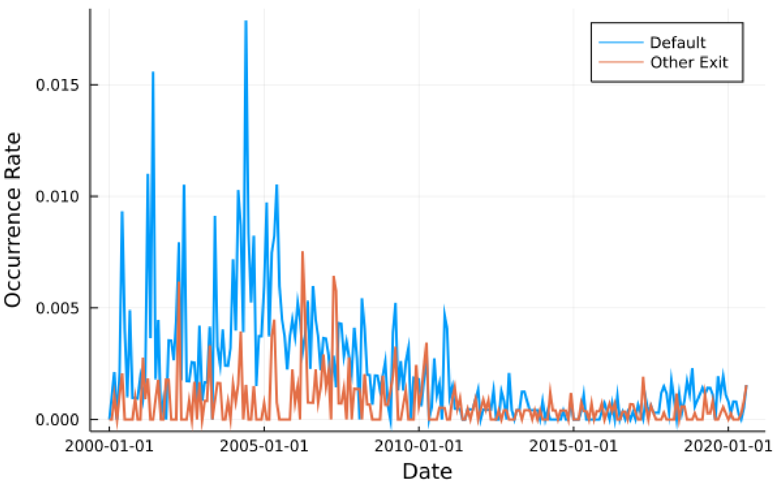
Figure 1 shows the monthly occurrence rate of default and other exit of Chinese-listed firms from 2000 to 2020. The occurrence rate is the frequency, i.e., the percentage of all active firms that defaulted or exited for other reasons. In general, Chinese-listed companies’ default events were shown to be more than other exits. Before 2011, the default monthly frequency was relatively high, peaking at over 1.5%. After 2011, the overall default frequency began to decrease and remained below 0.25% for the whole period.
Figure 2 shows the monthly occurrence rate of default and other exits of Chinese-listed firms for 7 months to 20 years following their first default. The situation within 6 months after a firm’s default is complex and is excluded from the sample. It is clear to see that in the 100 months following the first default, the default probability is significantly higher than the average default rate and gradually decreases as time goes by. Moreover, firms that have defaulted are more likely to default again or experience other type of exits in the future as compared with the average. The original method did not take this into account, which leads to deviations in predictions concerning firms in emerging markets such as China.
On the other hand, for all firms that have defaulted, if they do not exit the market, the probability of re-defaulting decreases over 10 years as the firm continues to operate.
We believe that the tendency to re-default decreases the longer the firm remains in business. In other words, the default heterogeneity of firms is also changing. We use Bayesian estimation to capture this. The PDs estimated using the original method were adjusted according to the past default status of the firm. Note that we still follow the assumption that the occurrences of default obey a doubly stochastic Poisson process proposed by Duffie et al. [3]. For each firm, if its default heterogeneity does not change, the number of defaults is still an independent incremental process, which means the time of each default does not affect the probability of future defaults. The change in the PD is mainly attributed to the change in the default heterogeneity of the firm. Moreover, among all firms that default, the frequency of other exits is more uniform over all future periods and significantly higher than that of other firms with a good credit status. For this near uniform frequency change, we added a state variable of whether the firm has defaulted into the variables of the other exit intensity function.
To check the out-of-sample performance, we divided the samples into an experimental group and evaluation group at a ratio of 5 to 1. After removing firms with too much missing data or too short a survival time, we were left with 4216 active firms. We randomly selected 3513 firms to form the experimental group in order to estimate the parameters, and we took the remaining 703 firms as the evaluation group to test the out-of-sample predictive ability.

5. Empirical Results

5.1. Parameter Estimates

We estimated γ l and δ l with horizon l from 0 month to 35 months by performing maximum pseudo-likelihood estimation on the experimental group sample. Table 3 and Table 4 show several representative prediction horizons for γ l and δ l :
We only discuss the new variable default record that the original model did not use. According to function 24, if a firm has defaulted, the forward other exit intensity will be more than 1.6 times higher than others in the same period. If we ignore this information, the POEs of a firm with one more default will be underestimated. Because the firm’s POE also affects the PD, it is important to consider the firm’s past default status. With γ l and δ l , we compute all firms’ default and other exit forward intensities, which are taken as the prior intensities. Then, we perform maximum pseudo-likelihood estimation on all listed samples to estimate β l using our model.
Table 5 shows β l for all the horizons that we estimated. According to Formula (20), the higher the β l , the greater the influence the prior PD has on the posterior PD. On the contrary, the firm’s past default situation affects the posterior PD more. From the estimation results, the past default situation has a higher impact on the short prediction horizon. As the prediction horizon increases, the influence of the prior PD on the posterior PD increases. If the firm has been in operation for a short time and has not defaulted, the PD is not changed much. For firms that have defaulted more than once, the adjusted posterior PD will be higher. On the contrary, if the company does not default for a very long time, the adjusted posterior PD will be lower. Moreover, PDs for shorter default horizons will be adjusted to a greater relative extent.

5.2. Prediction Accuracy Ratio

We employed Moody’s accuracy ratio as the assessment method, which is widely adopted in academia and industry to evaluate the predictive ability of posterior PDs. The accuracy ratio of the “perfect” model is 1, and the accuracy ratio of the zero-information model is 0. Readers may refer to Vassalou and Xing [26] for a more detailed description. If the accuracy ratio is above 0.5, the model contains a substantial amount of information. Figure 3 and Figure 4 show the cumulative accuracy profiles of the two groups.
We computed the cumulative accuracy using the out-of-sample’s (703 firms) monthly PD and real defaults in 240 months for the prediction horizons from 1 to 36 months and show the cumulative accuracy profiles for the following horizons: 1, 2, 3, 6, 12, 24, and 36 months. If the cumulative accuracy profile is a y = x line, the model has zero information. The larger area above the y = x line, the more defaults are captured. Figure 3 and Figure 4 show that our measure contains substantial information about future defaults both in and out of sample assessments.
When the prediction horizon is within 1 year, the prediction accuracy inside and outside the sample is very close. The accuracy ratio within 1 year was relatively high. When the prediction level was more than 2 years, the prediction ability of the model decreased. However, the model still maintained a strong prediction ability. The comparison of the accuracy ratio of the PDs before and after the adjustment for the 703 firms out of sample is shown in Table 6. This table shows the accuracy ratios of the revised PDs and the original PDs. The original PDs are estimated using the forward intensity model proposed by Duan et al. [1]. We employed Bayesian estimation on the default intensity estimated using the forward intensity model to estimate the posterior default intensity and calculate the revised PDs. We removed firms with less than 30 months of data. Figure 4 reports the out-of-sample results for the sample period 2000.01–2019.12. To compare the revised and original PDs, we divided the accuracy ratio of the revised PDs by that of the original PDs and then subtracted 1. Generally, the increased accuracy ratio of the out-of-sample revised PDs improved by almost 15% for prediction horizons of less than half a year. The accuracy ratio increased above 10% when the prediction horizons exceeded 1 year to 3 years. This shows that for Chinese-listed firms, introducing the heterogeneity of firms through Bayesian estimation can improve the accuracy of multi-period default prediction. The PDs adjusted by our Bayesian model can provide more information about future defaults.

5.3. Revised PDs of Firms with Default out of Sample

We found that there were 42 firms that defaulted in the 703 firms out of the sample for the sample period 2000.01–2019.12 and there were 70 defaults in total. We then selected all the firms that had defaulted and calculated their average cumulative PDs for all prediction horizons (1 month to 36 months). Figure 5 shows the revised PDs of firms with defaults compared with the average PDs. We found these firms’ average cumulative PDs to be approximately 4 times as much as all firms’ average cumulative PDs when prediction horizon is low. The revised average cumulative PDs of firms with defaults are always two times higher than other firms’ for all prediction horizons. Figure 6 shows the ranking of the revised average cumulative PDs of firms with defaults for all 703 firms. We found that these firm’s PDs were highly ranked. The model performance decreased a little when the prediction horizons increased. However, the defaulted firm’s average cumulative PDs were still in the top 5.5%. Obviously, our model can help practitioners identify firms with a high credit risk.

6. Conclusions

To address the problem of the large default heterogeneity of Chinese-listed firms, we conducted multi-period default prediction based on the forward intensity approach. Firstly, the default heterogeneity of Chinese-listed firms was introduced into the forward intensity model, and information concerning past defaults was taken into account. We employed Bayesian estimation to estimate the posterior default intensity. Maximum pseudo-likelihood estimation was conducted on the 3513 firms’ PDs to estimate the parameters of the Bayesian model. Finally, we rearranged the revised PDs for all prediction horizons to calculate the accuracy ratio. Through theoretical modeling and data analysis, we reached the following conclusions:
(1)
We found that the PDs or POEs of the firms with default records were significantly higher than the average level. The prediction performance of the forward intensity model can be improved by introducing firm’s default heterogeneity with information concerning a firm’s past default situation;
(2)
Bayesian estimation can help measure a firm’s default heterogeneity. By applying Bayesian estimation to a reduced-form credit risk model such as the forward intensity model, the original model can be optimized and the information of firm default heterogeneity can be taken into account to improve the prediction accuracy;
(3)
The empirical results show that the PDs revised by Bayesian estimation are higher than the original PDs of the original forward intensity model. For all prediction horizons, the accuracy ratio of the revised PDs out of sample increased by more than 10% as compared to the original PDs. Moreover, the accuracy ratio increased by almost 15% for prediction horizons of less than 6 months.
The main contribution of this paper is combining Bayesian estimation with the forward intensity model and introducing the firm’s default heterogeneity into the forward intensity model. This results in the re-estimated default intensity containing more effective information than the original default intensity. We propose a scientific approach that combines the prior default intensity with the firm’s past defaults. For Chinese-listed firms with a large heterogeneity in particular, it is important to introduce default heterogeneity into the model. According to the concepts in this paper, introducing the firm’s default heterogeneity into a scientific and accurate credit risk model using Bayesian estimation is helpful to improve the credit risk measurement system in China.
Furthermore, we believe the default heterogeneity can be further expanded. For example, the nature of the firm or the industry that the firm is in can both be taken into account to enrich our Bayesian model. Other credit risk models can also be optimized using our model, and our model can be verified with data from more countries.

Author Contributions

Conceptualization, Z.N.; methodology, Z.N.; software, Z.N.; validation, Z.N.; formal analysis, Z.N.; investigation, Z.N.; resources, M.J.; writing—original draft preparation, Z.N. and W.Z.; writing—review and editing, Z.N. and W.Z.; supervision, M.J.; project administration, M.J.; funding acquisition, M.J. All authors have read and agreed to the published version of the manuscript.

Funding

This research was supported in part by the National Natural Science Foundation of China Grant No. 71831005 and No. 71502044.

Institutional Review Board Statement

Not applicable.

Informed Consent Statement

Not applicable.

Data Availability Statement

Our data source is the Credit Research Initiative (CRI) database of National University of Singapore.

Conflicts of Interest

The authors declare no conflict of interest.

Appendix A

Appendix A shows how to estimate the forward intensity model. Firstly, we performed maximum pseudo-likelihood estimation on Chinese-listed firms and obtained γ l and δ(l). We were able to compute the default and other exit forward intensity according to the following function, in accordance with the work of Duan et al. [1]:
h i m , n = exp γ 0 l + γ 1 l x i m , 1 + + γ a l x i m , a , h ¯ i m , n = exp   δ 0 l + δ 1 l x i m , 1 + + δ a l x i m , a ,
where l = n m + 1 and X i t m = x i t , 1 ,   x i t , 2 ,   ,   x i t , a is the vector of all common variables and firm-specific variables for the i-th firm in the m-th month. Exponential functions ensure that the intensity is non-negative. For specific estimation details, readers may refer to Duan et al. [1]. Then, we conducted maximum likelihood estimation on a large sample of Chinese-listed firms to estimate the parameters of the gamma distribution:
β = β 0 , β 1 , , β l m a x 1 .
here, β is composed by l m a x sets of vectors, where l m a x is the longest prediction horizon. We assume the firms are conditionally independent and give the pseudo-likelihood function for the horizon of l months:
L l β l , τ D , τ O E , X = m = 1 N 1   i = 1 I P ^ l β l , τ i , τ ¯ i , X i m ,
where N denotes the last month of the sample, I is the number of firms in the sample, and P ^ l β l , τ D i , τ O E i , X i m is a probability according to the actual situation of the firm i during the period from m τ to m i n N τ , m + l τ as defined in the following:
P ^ l β l , τ i , τ ¯ i , X i m = 1 t 0 i m , m i n τ i , τ ¯ i > m + l P t 0 i m , m i n τ i , τ ¯ i > m + l + 1 t 0 i m , τ i τ ¯ i , τ i m + l P t 0 i m , τ i τ ¯ i , τ i m + l + 1 t 0 i m , τ ¯ i τ i , τ ¯ i m + l P t 0 i m , τ ¯ i τ i , τ ¯ i m + l + 1 t 0 i > m P t 0 i > m + 1 m i n τ i , τ ¯ i m P m i n τ i , τ ¯ i m .
here , 1 c o n d i t i o n = 1 if the condition is satisfied, and 1 c o n d i t i o n = 0 if the condition is not satisfied. The first probability is the cumulative probability of survival. The second probability is the i-th firm’s forward PD. The third probability is the i-th firm’s forward POE. The fourth probability is that the firm has not entered the sample. The final probability is that the firm has exited from the sample before the observation time. We combined the Formulas (23), (25), (27), (28), (29) and the above formula:
P ^ l β l , τ i , τ ¯ i , X i m = 1 t 0 i m , m i n τ i , τ ¯ i > m + l × exp { τ j = 0 l 1 [ β l + m l + 1 m 0 i m 0 i + l 1 m 1 y i s τ s = m 0 i m l h i s , s + l 1 β l + m l + 1 m 0 i h i m , m + j + h ¯ i m , m + j ] } + 1 t 0 i m , τ i τ ¯ i , τ i m + l 1 exp τ β l + m l + 1 m 0 i m 0 i + l 1 m 1 y i s τ s = m 0 i m l h i s , s + l 1 β l + m l + 1 m 0 i h i m , τ i × exp { τ j = 0 τ i m 2 [ β l + m l + 1 m 0 i m 0 i + l 1 m 1 y i s τ s = m 0 i m l h i s , s + l 1 β l + m l + 1 m 0 i h i m , m + j + h ¯ i m , m + j ] } + 1 t 0 i m , τ ¯ i τ i , τ ¯ i m + l 1 exp τ h ¯ i m , τ ¯ i × exp τ β l + m l + 1 m 0 i m 0 i + l 1 m 1 y i s τ s = m 0 i m l h i s , s + l 1 β l + m l + 1 m 0 i h i m , τ i × exp { τ j = 0 τ ¯ i m 2 [ β l + m l + 1 m 0 i m 0 i + l 1 m 1 y i s τ s = m 0 i m l h i s , s + l 1 β l + m l + 1 m 0 i h i m , m + j + h ¯ i m , m + j ] } + 1 t 0 i > m + 1 m i n τ i , τ ¯ i m .
The above formula is an overlapped pseudo-likelihood function similar to the one in Duan et al. [1]. The difference is that we use our posterior default intensity as a replacement. After computing the other exit intensity of all firms at all times using the original model, we maintained the terms associated with β l :
P ^ l , β l β l , τ i , τ ¯ i , X i m = 1 { t 0 i m , m i n τ i , τ ¯ i > m + l } exp [ τ j = 0 l 1 β l + m l + 1 m 0 i m 0 i + l 1 m 1 y i s τ s = m 0 i m l h i s , s + l 1 β l + m l + 1 m 0 i h i m , m + j ] + 1 t 0 i m , τ i τ ¯ i , τ i m + l exp τ j = 0 τ i m 2 β l + m l + 1 m 0 i m 0 i + l 1 m 1 y i s τ s = m 0 i m l h i s , s + l 1 β l + m l + 1 m 0 i h i m , m + j × 1 exp τ β l + m l + 1 m 0 i m 0 i + l 1 m 1 y i s τ s = m 0 i m l h i s , s + l 1 β l + m l + 1 m 0 i h i m , τ i + 1 t 0 i m , τ ¯ i τ i , τ ¯ i m + l exp [ τ j = 0 τ ¯ i m 2 β l + m l + 1 m 0 i m 0 i + l 1 m 1 y i s τ s = m 0 i m l h i s , s + l 1 β l + m l + 1 m 0 i h i m , m + j ] × exp τ β l + m l + 1 m 0 i m 0 i + l 1 m 1 y i s τ s = m 0 i m l h i s , s + l 1 β l + m l + 1 m 0 i h i m , τ i + 1 t 0 i > m + 1 m i n τ i , τ ¯ i m .
As long as we maximize P ^ l , β l β l , τ i , τ ¯ i , X i m , L l β l , τ D , τ O E , X will be the maximum. Because the pseudo-likelihood functions of different prediction horizons do not affect each other, we can estimate the parameters for all prediction horizons separately.

Appendix B

Appendix B shows gradient descent of pseudo log-likelihood function of adjusted default intensity. We performed Bayesian estimation with all the default forward intensities estimated using the original method. h i m , n denotes the i-th firm’s default forward intensity in month n, which was predicted in month m. Then, the forward default intensity of surviving, default, and other exit observations are as follows:
h i 0 m , n = 1 E i n = 0 × h i m , n h i 1 m , n = 1 E i n = 1 × h i m , n h i 2 m , n = 1 E i n = 2 × h i m , n ,
where E i n denotes the event of the i-th firm in month n. E i n = 0 means there is no default or other exit in month n for firm i. E i n = 1 means there is a default in month n, and E i n = 1 means there is an other exit event in month n.
Let I be the total number of firms and M be the total number of months observed. Then, the pseudo log-likelihood function of adjusted default probabilities for horizon l are expressed as follows:
L l = l n P l β , τ D , τ O E , X = τ i = 1 I m = m 0 i + l + 29 M i β l + m l + 1 m 0 i m 0 i + l 1 m 1 y i s τ s = m 0 i m l h i s , s + l 1 β l + m l + 1 m 0 i h i 0 , 2 m , m + l 1 + i = 1 I 1 m = m 0 i + l + 29 M i l n 1 exp τ β l + m l + 1 m 0 i m 0 i + l 1 m 1 y i s τ s = m 0 i m l h i s , s + l 1 β l + m l + 1 m 0 i h i 1 m , m + l 1
We take the derivative of L l and obtain the gradient:
G l = τ i = 1 I m = m 0 i + l + 29 M i m l + 1 m 0 i m l + 1 m 0 i m 0 i + l 1 m 1 y i s τ s = m 0 i m l h i s , s + l 1 ( β l + m l + 1 m 0 i ) 2 h i 0 , 2 m , m + l 1 + τ i = 1 I 1 m = m 0 i + l + 29 M i exp G i 1 m , l 1 exp G i 1 m , l × m l + 1 m 0 i m l + 1 m 0 i m 0 i + l 1 m 1 y i s τ s = m 0 i m l h i s , s + l 1 ( β l + m l + 1 m 0 i ) 2 h i 1 m , m + l 1 ,
here
G i 1 m , l = τ β l + m l + 1 m 0 i m 0 i + l 1 m 1 y i s τ s = m 0 i m l h i s , s + l 1 β l + m l + 1 m 0 i h i 1 m , m + l 1 .
Then, we calculate the maximum value of L l using the gradient descent method to estimate β l for all prediction horizons.

References

  1. Duan, J.C.; Sun, J.; Wang, T. Multiperiod corporate default prediction—A forward intensity approach. J. Econom. 2012, 170, 191–209. [Google Scholar] [CrossRef]
  2. Zhang, X.; Ouyang, R.; Liu, D.; Xu, L. Determinants of corporate default risk in China: The role of financial constraints. Econ. Model. 2020, 92, 87–98. [Google Scholar] [CrossRef]
  3. Duffie, D.; Saita, L.; Wang, K. Multi-period corporate default prediction with stochastic covariates. J. Financ. Econ. 2007, 83, 635–665. [Google Scholar] [CrossRef] [Green Version]
  4. Kealhofer, S. Quantifying credit risk I: Default prediction. Financ. Anal. J. 2003, 59, 30–44. [Google Scholar] [CrossRef]
  5. Altman, E.I. Financial ratios, discriminant analysis and the prediction of corporate bankruptcy. J. Financ. 1968, 23, 589–609. [Google Scholar] [CrossRef]
  6. Beaver, W.H. Market prices, financial ratios, and the prediction of failure. J. Account. Res. 1968, 6, 179–192. [Google Scholar] [CrossRef]
  7. Ohlson, J.A. Financial ratios and the probabilistic prediction of bankruptcy. J. Account. Res. 1980, 18, 109–131. [Google Scholar] [CrossRef] [Green Version]
  8. Zmijewski, M.E. Methodological issues related to the estimation of financial distress prediction models. J. Account. Res. 1984, 22, 59–82. [Google Scholar] [CrossRef]
  9. Gredil, O.R.; Kapadia, N.; Lee, J.H. On the information content of credit ratings and market-based measures of default risk. J. Financ. Econ. 2022, 146, 172–203. [Google Scholar] [CrossRef]
  10. Luong, T.M.; Scheule, H. Benchmarking forecast approaches for mortgage credit risk for forward periods. Eur. J. Oper. Res. 2022, 299, 750–767. [Google Scholar] [CrossRef]
  11. Matanda, E.; Chikodza, E.; Kwenda, F. Fuzzy structural risk of default for banks in Southern Africa. Cogent Econ. Financ. 2022, 10, 2141884. [Google Scholar] [CrossRef]
  12. Bu, S.; Guo, N.; Li, L.F. Rating frailty, Bayesian updates, and portfolio credit risk analysis. Quant. Financ. 2022, 22, 777–797. [Google Scholar] [CrossRef]
  13. Zhang, M.; Zhang, J.T.; Ma, R.L.; Chen, X.D. Quantifying Credit Risk of Supply Chain Finance: A Chinese Automobile Supply Chain Perspective. IEEE Access 2020, 7, 144264–144279. [Google Scholar] [CrossRef]
  14. Liu, Y.X.; Li, F.; Yu, X.H.; Yuan, J.H.; Zho, D. Assessing the Credit Risk of Corporate Bonds Based on Factor Analysis and Logistic Regress Analysis Techniques: Evidence from New Energy Enterprises in China. Sustainability 2018, 10, 1457. [Google Scholar] [CrossRef] [Green Version]
  15. Ma, J.J.; Guo, Y.H.; Zhu, Y. An empirical analysis of loan default behavior and credit risk of county SMEs. Manag. World 2004, 5, 58–66+87. (In Chinese) [Google Scholar]
  16. Xiao, Z. Research on Credit Risk Rating System of commercial banks of SMEs. J. Southeast Univ. 2014, 16 (Suppl. S2), 33–36. (In Chinese) [Google Scholar]
  17. Zhang, L.; Deng, X. Study of Credit Risk for Capital-Intensive Industries Based on Logistic Model. Int. Conf. Inf. Manag. 2009, 3, 390–393. [Google Scholar]
  18. Wei, P. Research on Credit Risks of China Listed SMEs—Based on Logistic Model Empirical Analysis. Financ. Regul. Res. 2012, 1, 101–116. (In Chinese) [Google Scholar]
  19. Gao, G.; Wang, H.X.; Gao, P.B. Establishing a Credit Risk Evaluation System for SMEs Using the Soft Voting Fusion Model. Risks 2021, 9, 202. [Google Scholar] [CrossRef]
  20. Abedin, M.Z.; Chi, G.T.; Hajek, P.; Zhang, T. Combining weighted SMOTE with ensemble learning for the class-imbalanced prediction of small business credit risk. Complex Intell. Syst. 2022; ahead of print. [Google Scholar] [CrossRef]
  21. Zhang, X.; Zhao, Y.; Yao, X. Forecasting corporate default risk in China. Int. J. Forecast. 2022, 38, 1054–1070. [Google Scholar] [CrossRef]
  22. Shih, Y.C.; Wang, Y.; Zhong, R.; Ma, Y.M. Corporate environmental responsibility and default risk: Evidence from China. Pac.-Basin Financ. J. 2021, 68, 101596. [Google Scholar] [CrossRef]
  23. Liu, L.L.; Luo, D.; Han, L. Default risk, state ownership and the cross-section of stock returns: Evidence from China. Rev. Quant. Financ. Account. 2019, 53, 933–966. [Google Scholar] [CrossRef] [Green Version]
  24. Jing, J.B.; Yan, W.W.; Deng, X.M. A hybrid model to estimate corporate default probabilities in China based on zero-price probability model and long short-term memory. Appl. Econ. Lett. 2021, 28, 413–420. [Google Scholar] [CrossRef]
  25. Duan, J.C.; Wang, T. Measuring Distance-to-Default for Financial and Non-Financial Firms. Glob. Credit. Rev. 2012, 2, 95–108. [Google Scholar] [CrossRef]
  26. Vassalou, M.; Xing, Y.H. Default risk in equity returns. J. Financ. 2004, 59, 831–868. [Google Scholar] [CrossRef]
Figure 1. Monthly occurrence rate of default and other exits of Chinese-listed firms. Source: NUS-CRI database.
Systems 11 00018 g001
Figure 2. Monthly occurrence rate of default and other exits of Chinese-listed firms for the 7 to 240 months following default. Source: NUS-CRI database.
Systems 11 00018 g002
Figure 3. This figure shows the in-sample cumulative accuracy profiles of the revised PDs based on the experimental group (3513 firms) in the period 2000.01–2019.12 for different prediction horizons.
Systems 11 00018 g003
Figure 4. This figure shows the out-of-sample cumulative accuracy profiles of the revised PDs based on the evaluation group (703 firms) in the period 2000.01–2019.12 for different prediction horizons.
Systems 11 00018 g004
Figure 5. This figure shows the out-of-sample revised average cumulative PDs of the defaulted 42 firms in the period 2000.01–2019.12 as compared with the overall mean level for different prediction horizons.
Systems 11 00018 g005
Figure 6. This figure shows the ranking of out-of-sample revised average cumulative PDs of the defaulted 42 firms in the period 2000.01–2019.12 for all 703 firms out of sample for different prediction horizons.
Systems 11 00018 g006
Table 1. Common variables.
Common Variables Interpretation
1 Stock index return
2 Interest rate
3 Financial aggregate DTD
4 Non-financial aggregate DTD
Shanghai SE composite index
China time deposit rate, 3 months
median DTD of financial firms in China
median DTD of non–financial firms in China
Table 2. Firm-specific variables.
Firm-Specific Variables Interpretation
1. DTD (level)the 1-year average of distance-to-default (DTD)
2. DTD (trend)the current value of DTD minus level of DTD
3. CASH/TA (level)level of {ln[(cash + short–term investments)/total assets]} (only applies to financial firms)
4. CA/CL (level)level of {ln[(cash + short–term investments)/total assets]} (only applies to financial firms)
5. CA/CL (trend)trend of [ln(current assets/current liabilities)] (only applies to non–financial firms)
6. NI/TA (level)level of (net income/total assets)
7. NI/TA (trend)trend of (net income/total assets)
8. SIZE (level)level of [ln(firm market capitalization/China’s median market capitalization over the past 1 year)]
9. SIZE (trend)trend of [ln(firm market capitalization/China’s median market capitalization over the past one year)]
10. M/Bfirm’s M/B (current value)/China’s M/B median (current value)
11. SIGMAcurrent value of SIGMA is defined to be the standard deviation of the residuals of this regression
12. Default recordIf the firm has defaulted before, the value is 1, otherwise the value is 0. Only for the other exit intensity function.
Table 3. Parameters of the default forward intensity function.
γ 1 γ 2 γ 3 γ 6 γ 12 γ 24 γ 36
Intercept−3.19567−3.22324−3.14231−2.75779−3.35508−3.48794−5.61305
Stock Index0.3647040.3454550.371220.4955710.2954830.0363420.401967
Interest R−0.09484−0.14648−0.20179−0.26951−0.27651−0.48271−0.59288
DTD (L)−0.44485−0.43777−0.41021−0.37806−0.30378−0.23925−0.159
DTD (T)−0.24401−0.25766−0.24311−0.17357−0.15487−0.16768−0.11836
Liquidity (L)−0.35206−0.37554−0.3775−0.36836−0.36478−0.32862−0.35424
Liquidity (T)−0.21799−0.13562−0.20819−0.36271−0.2559−0.677510.370419
NI/TA (L)−27.1892−27.5629−29.3298−34.5291−49.0559−17.5311−11.7268
NI/TA(T)−3.86283−5.04577−3.951471.6056391.843335−6.48836−0.6641
Size (L)−0.58644−0.58365−0.55998−0.53765−0.30256−0.123170.034523
Size (T)−0.80865−0.78113−0.71216−1.01524−0.64005−0.41534−0.43872
M/B0.0005310.0021970.005594−0.01068−0.026530.0400470.029517
SIGMA0.9079690.815252−0.09427−2.19432−0.9430.9953370.990411
DTD median 0.1530460.1731950.176920.1113550.1494620.120510.460361
Table 4. Parameters of the other exit forward intensity function.
δ 1 δ 2 δ 3 δ 6 δ 12 δ 24 δ 36
Intercept−5.15746−4.60163−4.52391−3.51009−3.91152−5.01547−5.34153
Stock Index0.4344840.4510390.3810080.4106610.0688860.432342−0.02859
Interest R−0.07809−0.10849−0.13178−0.10656−0.031380.1827220.265114
DTD (L)−0.14544−0.16673−0.1723−0.13182−0.042590.012357−0.03725
DTD (T)0.1643780.0852480.03270.016497−0.13590.135816−0.09274
Liquidity (L)−0.18405−0.17164−0.16201−0.08269−0.10729−0.03911−0.0625
Liquidity (T)−0.47692−0.27531−0.35687−0.64659−0.80462−0.681530.217479
NI/TA (L)−36.8954−35.3574−36.5993−33.0425−44.9344−42.5486−35.9121
NI/TA(T)−1.824020.4976582.6199568.891169−1.08149−3.4806−2.80377
Size (L)−0.1468−0.15416−0.15002−0.111280.0125860.033836−0.01243
Size (T)−0.02591−0.05804−0.39226−0.19978−0.394790.5191961.02308
M/B0.0016920.0302780.0239470.022703−0.05535−0.06474−0.0949
SIGMA4.6986932.554482.9671650.175135−0.74486−0.804690.271515
DTD median −0.00836−0.04844−0.05661−0.27929−0.24043−0.14105−0.06458
Default or not 1.1793761.1726371.1862721.1693661.0609420.8642980.766159
Table 5. Parameters of the Bayesian model.
Maximum   Pseudo - Likelihood   Estimates   for   β l :   1 36   Months
β 1 β 2 β 3 β 4 β 5 β 6 β 7 β 8 β 9
226.581238.277269.5841279.075322.4939357.731390.9475471.209498.9649
β 10 β 11 β 12 β 13 β 14 β 15 β 16 β 17 β 18
517.6742577.8831654.2477621.2871593.5402693.7856659.347727.2746698.5131
β 19 β 20 β 21 β 22 β 23 β 24 β 25 β 26 β 27
763.7637922.96531200.171240.0381179.6481167.2291218.5841107.113976.984
β 28 β 29 β 30 β 31 β 32 β 33 β 34 β 35 β 36
1076.0281198.7351166.1151075.318988.62971115.7031175.411270.0191331.149
Table 6. Comparison of the accuracy ratios.
Accuracy Ratio 1 Month2 Months3 Months6 Months12 Months24 Months36 Months
Original PDs0.58820.58760.60320.59020.56960.52690.5161
Revised PDs0.67600.67660.69310.69050.63780.59960.5775
Increased (%)14.915.214.917.012.013.811.9
Disclaimer/Publisher’s Note: The statements, opinions and data contained in all publications are solely those of the individual author(s) and contributor(s) and not of MDPI and/or the editor(s). MDPI and/or the editor(s) disclaim responsibility for any injury to people or property resulting from any ideas, methods, instructions or products referred to in the content.

