Article

Optimization of a Rural Portfolio Credit Granting System Using Improved Two-Dimensional Strip Packing Grouping Delay Problem

1
School of Politics and Public Management, Guangxi Minzu University, Nanning 530006, China
2
School of Computer Science and Engineering, Huizhou University, Huizhou 516001, China
*
Author to whom correspondence should be addressed.
Systems 2022, 10(5), 193; https://doi.org/10.3390/systems10050193
Submission received: 20 August 2022 / Revised: 14 October 2022 / Accepted: 18 October 2022 / Published: 21 October 2022

Abstract

:
Rural preferential loans usually take the form of portfolio credits. From the perspective of public interest, the total delay time for obtaining loans is expected to be minimized. To use rural portfolio credits effectively, the two-dimensional strip packing grouping delay problem (2SPGDP) is improved to optimize the rural portfolio credit granting system. First, 2SPGDP is established by adding grouping constraints and the latest start time constraints to the two-dimensional strip packing problem, and the total delay is taken as the optimization objective. Second, based on the depth search reverse spanning tree (DSRST) and the insert spare space (ISS) method, the branch-and-bound reverse order insert algorithm (BB-RIA) is designed. Finally, the lag pruning operator (LPO) is designed to reduce lag. The improved model (2SPGDP) and BB-RIA-LPO algorithm are used to solve several classical two-dimensional strip packing problems and a specific rural portfolio credit case. Compared with the Bottom-Left and Branch and Bound Algorithm, our model and algorithm improve the success rate by 25% and reduce the total delay by 6%. The case of rural portfolio credit illustrates the operability and effectiveness of this method.

1. Introduction

Rural referential finance is a requirement by the government regarding the public interest and social responsibility of rural financial institutions. Rural commercial banks will set favorable terms to enable villagers and rural small businesses to obtain preferential loans and increase their satisfaction with the government [1]. Rural preferential credit has many forms, among which “whole village credit” is a new rural portfolio credit method of “whole village wholesale centralized credit” established in the process of “batch credit, self-help lending, without guarantee”, aiming to meet the needs of the rural financial granting system [2,3,4,5,6]. In the rural portfolio credit plan project, the risk control mechanism is set for each village. When the nonperforming loan rate of a village is higher than 3%, village credit is stopped; if it is less than 3%, the loss will be shared by the guarantee company established by the government and the bank to ensure the progress of the planned project. If a strip box is set, the height is the total amount of rural portfolio credit of rural commercial banks, and the length is time. Due to the risk control mechanism, this paper does not consider the reduction of the total amount of loans caused by nonperforming loans, that is, the reduction of the height of the box. The loan items are grouped according to their villages to generate group constraints. The latest loan-obtaining time for each village is set to be the same. Each loan item is a rectangle, with the height and length representing the loan amount and loan term, respectively, and the final optimization target is the total loan-obtaining time delay. Then, the rural portfolio credit scheduling problem is abstracted as a two-dimensional packing problem with the goal of group constraints and total delay time, which is called the two-dimensional packing grouping delay problem in this paper (2SPDGP). Solving such problems can solve the problem of capital occupation of rural commercial banks, achieve collective management through village credit, reduce risks, optimize the total delay time, improve satisfaction, and promote the sustainability of rural portfolio credit financial systems. Figure 1 shows the credit relationship between the government, the village committee, and the villagers. The government gives credit to the rural commercial bank, and the rural commercial bank gives credit to the village committee and directly makes and recovers loans to the villagers. The village committee and the rural commercial bank jointly manage the loan item of villagers.
In recent years, many studies and applications have been conducted on the algorithm of the two-dimensional packing problem (2SPP) [7]. Deterministic algorithms mainly use models to construct accurate solutions or improve the branch pricing method to improve the optimization ability and efficiency of the algorithm. Cid-Garcia et al. [8] used the location and coverage method to obtain the two-dimensional, non-guillotine-constrained 2SP exact solution, generated a set of effective locations in the form of pseudo polynomials, and selected the best configuration of the strip box items by using the set coverage formula. Qi et al. [9] studied the relationship between the lower left coordinates of the rectangles and strip boxes and established linear integer programming models of nonrotating and rotating two-dimensional rectangular strip boxes to ensure that the two rectangles would not be placed repeatedly. Queiroz [10] presented a tailored branch-and-cut algorithm for the two-dimensional irregular strip packing problem with uncertain demand for the items to be cut. A two-stage stochastic programming model is developed, considering a discrete and finite set of scenarios. However, precise algorithms rarely study the problem of taking delay as the optimization goal. The heuristic algorithm is fast and can obtain the local optimal solution. Oviedo-Salas et al. [11] proposed an improved greedy random adaptive search process (GRASP) in which three loss functions are used as the alternative objective functions of the GRASP candidate list, and overlapping functions are used to ensure that the object is suitable for labelling; this method shows improved performance compared to other metaheuristic algorithms. Wei et al. [12] proposed an improved heuristic algorithm based on Best-Fit that used adaptive values to select the best rectangle suitable for the gap, providing an efficient implementation mode with O(n log n) time complexity for the improved heuristic algorithm of the best fit. By trying different sequences, a simple random local search was used to improve the results. Chen and Chen [13] presented a corner increment-based algorithm for solving the two-dimensional strip packing problem without the guillotine constraint; it adopted heuristics in the corner increment strategy, segment tree, and multistart random local search. Chen et al. [14] proposed a variant of a hybrid heuristic algorithm for optimizing solutions to the strip packing problem; they adopted scoring rules for selecting rectangles and used red-black trees that store rectangle indices and random local search. A genetic evolutionary algorithm is often used to improve the efficiency of a solution. Li et al. [15] proposed the hybrid adaptive genetic algorithm (HAGA) for solving the NP-hard two-dimensional rectangular packing problem to maximize the filling rate of a rectangular sheet. Mondal and Tsourdos [16] presented a two-dimensional quantum genetic algorithm (2D-QGA), which is a new variety of QGA. Recently, reinforcement learning has been added to the two-dimensional packing problem. Neuenfeldt et al. [17] adopted supervised machine learning techniques to select multilabel dataset transformation for solving metal and paper roll shearing problems in industrial processes that improved the solution accuracy compared with other improved heuristic algorithms. Although many heuristic and evolutionary computing methods can improve the efficiency of the solution, these algorithms introduce random numbers, and the solution is uncertain in the same case. In the actual operation of bank portfolio credit, it is easy to cause disputes among lenders, so it is not applicable. There are also some applications in the field of economic management on the two-dimensional packing problem. Zheng et al. [18] study a realistic aircraft scheduling and parking problem with the goal of simultaneously determining the takeoff and landing time of each aircraft with consideration for wake vortex effect constraints and parking positions in the limited parking apron at a target airport. However, there are few applications in the field of bank credit. The 2SPP literature review also mentions the classification of various constraints. Vega-Mejia [19] provides an overview of recent optimization developments for integrating packing and routing problems to propose a simple classification scheme for realigning the optimization criteria and operational constraints, taking into consideration the issues of sustainability. Júnior et al. [20] conducted a literature review of current 2SP problems in practical problem constraints. These reviews discussed most of the constraints but did not address combinatorial constraints and the latest start length constraint. In additional, there is an exponential relationship between the computational cost and the problem size of the two-dimensional packing problem algorithm [21].
In summary, among the literature on 2SPP, there are few studies on the delay time objective in deterministic solution methods. Due to the uncertainty of the solution results under the same conditions, many heuristic evolutionary hybrid algorithms are not applicable to bank portfolio credit, which easily causes controversy. The application of 2SPP in the field of bank credit is rare. There are few studies on combinatorial constraints and fairness strategies. Starting from the bank portfolio credit problem, this paper abstracts the two-dimensional strip packing mathematical problem of grouping (combinatorial constraints) and delay optimization for research. First, the two-dimensional strip packing problem is modified based on the bank portfolio credit problem. By adding the group credit, the latest start time and the total delay corresponding to the bank portfolio credit problem as the grouping constraint, the latest start length, and the delay optimization goal, a two-dimensional strip packing grouping delay optimization problem (2SPGDP) is established. Second, based on the deep search reverse spanning tree (DSRST) and the insertion spare space (ISS) operator, a branch-and-bound reverse order insert algorithm (BB-RIA) is designed to cover the state of most of the decomposition space and effectively use the free space of the strip box. Third, a lag pruning operator (LPO) is designed for the goal of delay optimization, which can be used as an optimization criterion to obtain a better solution. Finally, the improved classical test examples and a specific case are used to verify the effectiveness of the algorithm.

2. Problem Description and Mathematical Model

In this section, we abstract the rural portfolio credit scheduling problem into the 2SPGDP scheduling problem and provide a simple example.

2.1. Problem Description

Table 1 lists the symbol descriptions for the problem and the meaning in the rural portfolio scheduling problem. If a strip box has a certain height H and infinite length, there are g rectangle groupings represented by Gk, k ∈ {1,2, …, g}, each rectangle group has mk rectangles, represented by Rki,i ∈ {1,2, …, mk}, and the height and length of the rectangle Rki are hki and lki, respectively. hki < H, lki is a limited value and integer. R is the set of all rectangles, R = { R k i | k = 1 , 2 , , g , i = 1 , 2 , , m k } , which are the rectangular schedules in the strip box. The start and end lengths of each rectangular schedule are SLki and ELk, respectively. Each set of rectangles has the latest starting length constraint LSLki. If it is longer than this length, the penalty function will be calculated based on the delay length. The delay length is defined as the difference between the rectangle start length SLki and the latest start length LSLki after scheduling. If the delay length is negative, it means there is no delay. If it is positive, it is included in the delay, as shown in the following equation:
D L k i = { S L k i L S L k i , if   S L k i L S L k i > 0 0 , if   S L k i L S L k i 0
The rectangle grouping constraint, defined as the sum of the heights of the same group of rectangles, cannot exceed the height of the constraint at the same length position, as shown in the following equation:
i = 1 m k h k i , h k i [ S T k i , E T k i ) I i = 1 m k h k i G H C k i
The optimization goal of the scheduling problem is to calculate the minimum sum of all delay lengths under rectangular grouping constraints, as shown in Equation (3):
D L = min k = 1 g i = 1 m k D L k i
The goal of the scheduling problem was to minimize the sum of the total scheduling delay times DL.

2.2. Simple Example

The following content will illustrate the process of abstracting the rural portfolio credit scheduling problem into 2SPGDP with a simple case: A bank’s total amount of rural portfolio credit is limited to 6 million yuan, and villages 1 and 2 participate in the portfolio credit project. In the first village, three villagers borrow money, with credit lines of two, two, and one million yuan, and the terms are two years, one year, and two years, respectively. The latest loan-obtaining time in this village is 0.2 years, and the credit for the whole village is 4 million yuan. In the second village, two villagers’ loan amounts are two million yuan and one million yuan, with terms of two years and one year, respectively. The latest loan-obtaining time for this village is 0.4 years, and the credit for the whole village is 3 million yuan. We abstract the village as a group k, the total credit H = 6, the villagers’ loan item is abstracted as rectangular Rki, the loan amount is abstracted as hki, the loan term is abstracted as lki, the latest loan obtaining time is abstracted as LSLk, and the credit of the village is abstracted as GHLk. See Table 2 for details.
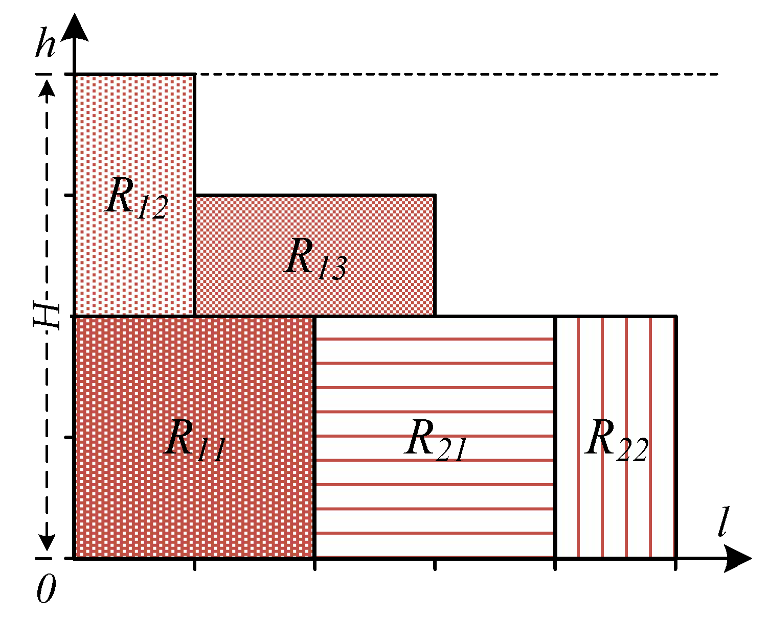
Figure 2 is a simple example of 2SPGDP scheduling. Compared with the classical packing problem, we rotate the box 90° clockwise and transform the width W and height H of the classical box into H and L described in this problem. According to the Bottom-Left algorithm, we first find the minimum length, then we find the coordinate point of the minimum height as the placement point and place the point at the bottom left corner of the rectangle at the placement point. We complete the scheduling according to the order and constraints in the table. In the figure, we can see that R22 does not place a point according to the BL algorithm because of the constraints of this group of heights GHL2.
Finally, we determine all the scheduling start times SL11, SL12, SL13, SL21 and SL22 as 0, 0, 1, 2, and 4, respectively. According to Equation (3), we calculate the total delay
D L = k = 1 g i = 1 m k D L k i = 0 + 0 + ( 1 0.2 ) + ( 2 0.4 ) + ( 4 0.4 ) = 5.2
Therefore, there is a total delay time of 5.2 years when switching to rural portfolio credit.

2.3. Mathematical Model

This subsection presents a mixed-integer programming model for the two-dimensional strip packing grouping delay optimization problem (2SPGDP). This problem is based on five assumptions as follows [22]:
(1)
All rectangles must be packed into a strip box.
(2)
The sides of the rectangle must be parallel to the strip box, that is, right-angle filling.
(3)
The rectangle cannot be rotated.
(4)
Any two rectangles cannot overlap.
(5)
One size fits all must not be a requirement.
There are several rectangles R(xri,yri) in rectangle group Gr, and (xri,yri) is its minimum coordinate after scheduling, namely:
x r i = min { p | p [ x k i , x k i + l k i ) , p I } ,   y r i = min { q | q [ y k i , y k i + h k i ) , q I }
Additionally, I is a set of natural numbers. To schedule them in the strip box with height H and length L that has infinite length, all rectangles should be scheduled. The model aims to minimize the sum of the delay lengths. Since all rectangles must be scheduled, the description of the rectangles Rri and Rsj according to Scheithauer’s mixed linear integer model based on mutual positions is defined through the binary variables uri,sj and vri,sj. If r = s then ij, i, j, r, sI; then, the mathematical model is given by:
z = min k = 1 g i = 1 m k D L k i   s . t .
0 x r i L l r i , 0 y r i H h r i , r , i I ,
x r i + l r i x s j + L ¯ ( 1 v r i , s j ) ,   y r i + h r i y s j + H ( 1 v r i , s j ) ,   i , j , r , s I ,   i f   r = s   t h e n   i j
u r i , s j + u s j , r i + v r i , s j + v s j , r i = 1 ,   i , j , r , s I ,   i f   r = s   t h e n   i j
u r i , s j , v r i , s j { 0 , 1 }   ,   i j ,   i , j , r , s I ,   i f   r = s   t h e n   i j
i = 1 m k h k i ,   h k i [ S T k i , E T k i ) I ,   i = 1 m k h k i G H C k
L ¯ Z + is the length of a feasible scheduling pattern, Z+ is a positive integer, and I is a natural number. Condition (6) states that all rectangles Rki(xki,yki) are placed in a horizontal strip box of height H and length L. According to Condition (5), the optimization goal is to minimize all delay lengths. Condition (8) ensures that the position relations between any two pairs of rectangles can only be one of the four directions, namely, the determinable variables uri,sj, usj, ri, vri,sj, and vsj,ri, and only one of the four position relations can be equal to 1. Condition (7) indicates that all rectangles will not overlap horizontally or vertically; this model can also be taken as a Padberg-type model due to the use of binary variables. The grouping constraint scheduling policy has constraints on the sum of the scheduling lengths for all rectangles belonging to the same group. Grouping constraints are used to limit the total height of a group of items of the same length. Equation (9) indicates that the value of the binary variable of the relationship is either 0 or 1. Constraint (10) is a grouping constraint. If all rectangles in the same group are scheduled at the same length, their sum at this length cannot be more than GHCk.
It should also be considered that the number of binary variables is either too large to be solved by standard computer software for strip packing problem (SPP) instance problems or too computationally expensive to be solved. In any case, the model provides a lower bound of optimized length or an approximate solution.
The natural lower bound of the grouped SPP model can be deduced as follows. Due to the grouping constraint, regardless of the location of the rectangle, the natural lower bound of each group is given by:
L B G k = i = 1 m k h k i l k i / G H C k
Then, the natural lower bound of all rectangular group scheduling can be estimated as follows:
L B G = k = 1 g L B G k / H = k = 1 g i = 1 m k h k i l k i / H

2.4. Lower Bound of Group Fairness

Figure 3 shows an example of calculating the delay time score. In this paper, we consider the fairness policy in the same group; that is, intragroup fairness is considered. The latest start time LSLk for each group is set to the first scheduled time of the tasks in the group.
Then, we can obtain the lower bound of the optimization target delay time by reasoning as follows. Our latest start time LSLk is 0. According to Equation (5), we calculate the delay time in Figure 3a–d. The delay time is DLa = 3 × (1 + 2) = 9, DLb = 3 × (1 + 2) − 1 = 8, DLc = 3 × (1 + 2) − 2 = 7, and DLd = 1 × 2 + 2 × 1 = 5.
Therefore, we derive the formula of arbitrary rectangular scheduling to reduce the calculation delay:
D L = j = 1 E L g m g j × h k i ( j = S L k i L L C k E L k i L L C k i j ) × h k i + ( S L k i L L C k )
Proof: Suppose there is a strip box of width W and unlimited length, each rectangle is a unit rectangle, and the latest start time of all rectangles is 0, then the maximum delay generated by all rectangles is:
D L U B = j = 1 E L g m g j × h k i
When an arbitrary rectangle Rki of the height hki and the length lki is scheduled, the maximum delay it can actually reduce is:
D L R k i = ( j = S L k i L L C k E L k i L L C k i j ) × h k i
Finally, it must add its own delay at the front, and that delay is ( S L k i L L C k ) , which concludes the proof.
D L = k = 1 g D L G k = k = 1 g [ j = 1 E L g m g j × h k i ( j = S L k i L L C k E L k i L L C k i j ) × h k i + ( S L k i L L C k ) ]

3. Branch and Bound Reverse Order Insert Algorithm

To solve the portfolio credit-granting problem, based on the two-dimensional strip packing grouping delay optimization problem (2SPGDP), we design a deep search reverse spanning tree (DSRST) to generate a solution space for minimizing the sum of the latest start time lag of all rectangles and consider fairness in the same group at the latest start time. An insert spare space (ISS) is used instead of a skyline [12] to insert new rectangles. The lag pruning operator (LPO) is used to cut off the lagging branches. Based on the improvements above, we design the branch-and-bound reverse order insert algorithm (BB-RIA) and consider the equivalence and dominance of the classical pruning strategy to improve the quality and efficiency of the solution. These methods are described in detail in this section.

3.1. Deep Search Inverse Spanning Tree (DSRST)

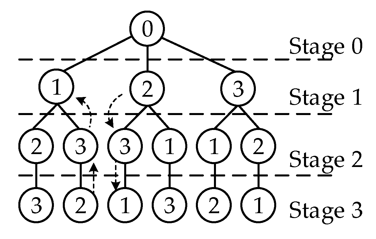
The algorithm is based on a deep search reverse spanning tree (DSRST) to generate a search space. This method can cover the states in most search spaces and avoid generating solution space state explosion. Figure 4 shows the deep search inverse spanning tree (DSRST) of three variables; the variables are 1, 2, and 3, and 0 is set as a pseudo variable (node) for exchanging the first variable. Starting from the leftmost branch, Stages 0–3 are searched in-depth in the order of 0-1-2-3; the second branch generating the third branch is taken as an example. The second branch backtracks from Stage 3 and pushes variables to Stage 1. In contrast, variable 2 at the top of the stack does not appear in Stage 1, so it starts from variable 2 of Stage 1 to variable 1 of Stage 3 in the deep reverse back stack to complete the generation of the third branch, as shown by the dotted line in Figure 4.

3.2. Insert Spare Space (ISS)

The appropriate position in the strip box is selected, and the new rectangle is scheduled using the insert spare space (ISS) method. Compared with the skyline method, the frequency of searches increases, but the waste of space is also reduced, and a better solution can be obtained.
The rectangle placement point is set as (x,y) and Rki(x,y) ∈ I to define the rectangle coverage:
R k i ( x , y ) : = { ( p , q ) R 2 : x p x + l k i , y q y + h k i }
A packing mode is defined as:
A ( I ˜ ) : = { R k i ( x k i , y k i ) : k i I ˜ }
For a related mode of packing, I ˜ I is a subset of the set of all of the rectangles. When all scheduled rectangles are placed left first and then right, this is called regularization or upper-left alignment. The contour of the A ( I ˜ ) mode is defined as:
U ( A ( I ˜ ) ) : = { ( x , y ) R + 2 : k i I , ˜   x x k i + l k i , y y k i + h k i }
To make the placement more compact, the placement point is designed as the contour corner point, which is the point aligned at the bottom left corner of the contour except for the origin (0,0):
S c o r p t = { ( x , y ) | ( x , y ) , ( x 1 , y 1 ) U ( A ( I ˜ ) ) ,       ( x > 0 y 1 = 0 ) [ ( y 1 = y 1 ) x 1 > x ] }
According to the coordinate axes in Figure 4, two boundary corner points are defined as:
p b o u H = ( x b o u H , H ) , x U ( A ( I ˜ ) ) , x b o u H = max ( x ) p b o u 0 = ( x b o u 0 , 0 ) , x U ( A ( I ˜ ) ) , x b o u 0 = max ( x ) x b o u = min ( x b o u 0 , x b o u H )
Xex-ctr-0 and Xex-ctr-H are the horizontal coordinate values of the intersection of the outer contours x = 0 and x = H, respectively, that is, the height boundary of the strip box. Xex-ctr is the minimum value of the two corner points. Then, we can define the set of outer contour placement points and inner contour placement points:
S p t e x = { ( x , y ) | ( x , y ) S c o r p t , x x e x c t r }
S p t i n = { ( x , y ) | ( x , y ) S c o r p t , x < x e x c t r }
Then, according to relevant definitions, it can be shown that the set of placement points of the outer contour is the set of placement points generated by the classical skyline, while the set of placement points of the inner contour is the set of points searched by the insert spare space method described in this subsection when the new rectangle is placed. Increasing the set of inner contour placement points increases the cost of the search calculation.
As shown in Figure 5, Rectangles R1, R2, and R3 are set with widths of 2, 1, and 1 and heights of 1, 2, and 1, respectively. The scheduling sequence is 1–3. In the problem of regularization scheduling in this paper, the point with the shortest length is considered first, and then the point with the lowest height is considered the starting point to schedule the current rectangle. When the scheduling of rectangle R3 is prepared, the skyline method seeks the scheduling placement point from the regularization position of the outer contour, that is, the position of the placement point is at (3,0), as shown in Figure 5a. The ISS method starts from the regularization integer point (0,0) to search for the scheduling placement point; thus, the point (0,1) searched is the scheduling placement point, as shown in Figure 5b. Therefore, the ISS method can save space.

3.3. Lag Pruning Operator (LPO)

For groups with different latest start times, it is necessary to consider the lag placement of some rectangles, that is, the shortest start time of some rectangles is later than the shortest start time of the current rectangle. However, in the strip box, the space is scheduled to be shorter than the length of the current rectangle. Therefore, we design a lag pruning operator (LPO) to improve the search ability, avoid being pruned in advance, and increase the search effect. Rki is set to be the current scheduling rectangle; hki and lki are the height and length, respectively; LSLk is the latest starting length.
Sa is the set of all rectangles in packaging mode A ( I ˜ ) , while Slag is the set of rectangles in packaging mode A ( I ˜ ) where there is a rectangle Rki, whose start time is greater than that of other rectangles SLki > SLpj, and the latest start length is less than that of other rectangles LSLk < LSLp. | S · | is the number of rectangles in the set and the lag factor Lf is defined as follows:
L f = | S l a g / S a | , S l a g = { R k i | R k i , R p j A ( I ˜ ) , ( L S L k i < L S L p j ) ( S L k i > S L p j ) }
Figure 6 is a schematic diagram of the lag relation and Rectangles R1, R2, and R3 in the previous section, whose latest start lengths are 0, 1, and 2, respectively.
Figure 6a shows that if the current scheduling rectangle is set to R3, the lag factor Lf = 0; if the current scheduling rectangle is set to R2, it is observed from Figure 6b that there are two rectangles with starting lengths longer than Rectangle R2; thus, Lf = 2/3. In the algorithm, the lag pruning operator evaluates whether the sum of the lag factors of each rectangle is greater than the set lag limit (LL) under the current packing mode, and LL ∈ (0,1). If it is greater than the lag limit, the pruning operation will be carried out.

3.4. Delay Equivalence and Dominance

In the branch-and-bound algorithm, equivalence and dominance relations are needed for pruning algorithmic spanning trees to reduce the computational cost. Relevant literature studies can be found in [22]. In this paper, equivalence and dominance are evaluated by the delay length as given by Equation (3).

3.5. Algorithm Flow

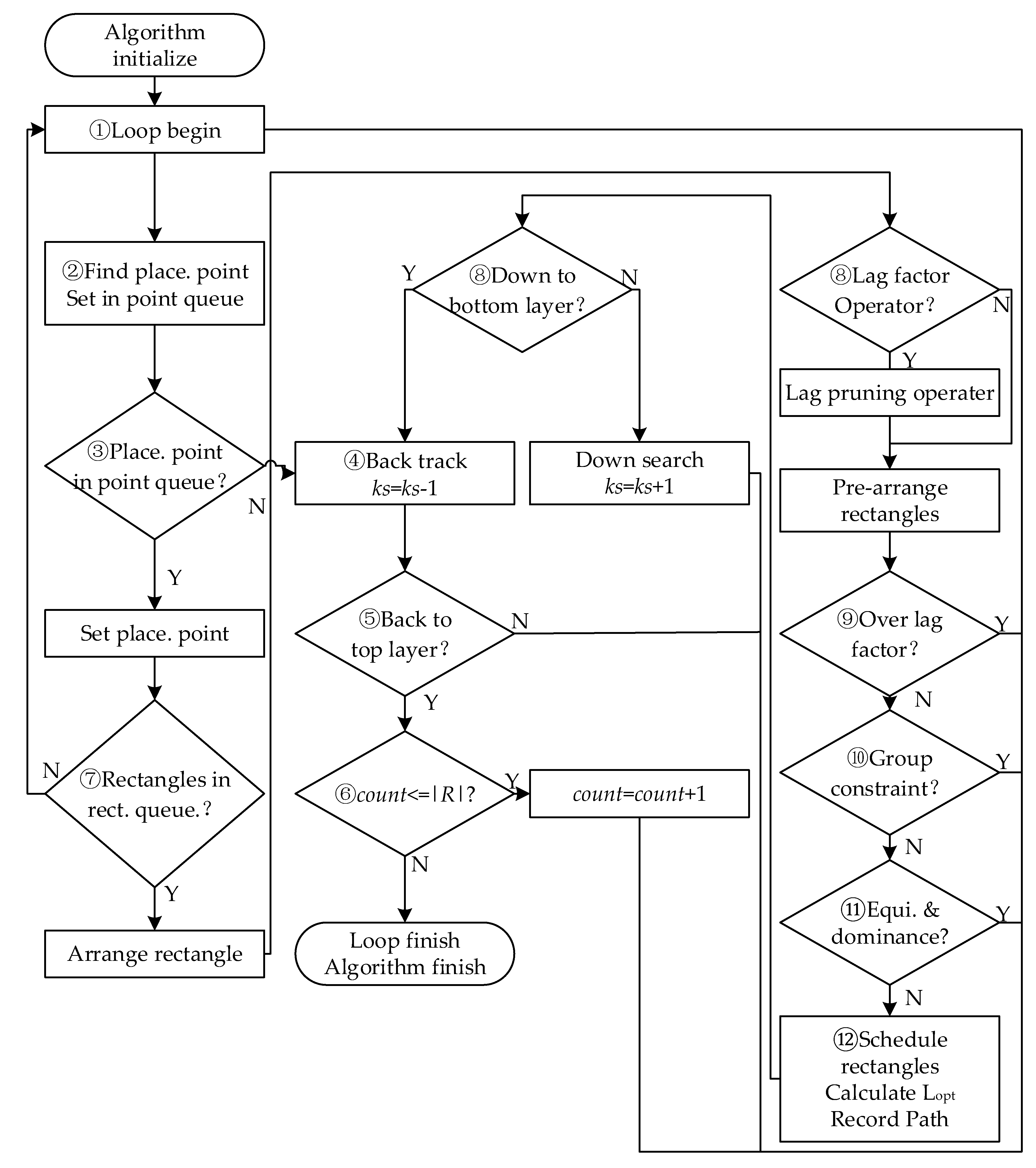
The operators introduced in this section will be used to generate the branch and bound reverse-order insert algorithm with the lag pruning operator (BB-RIA-LPO) algorithm. Table 3 shows the pseudocodes of the BB-RIA-LPO algorithm, where ks is the search depth, count is the number of times that ks is assigned to 0, and |R| is the number of all rectangles. Figure 7 shows the algorithm flowchart.
The two-dimensional strip packing grouping delay optimization problem (2SPGDP) and the corresponding latest start time LSLki, grouping constraint GHCk, rectangle height hki, and length lki are based on group fairness that set the latest start length equal to the same group LSLki = LSLk, (i = 1, 2, …, mk). The partial solution space is generated by a deep search inverse spanning tree. Using the branch-and-bound method, the placement point and the dispatch rectangle are found. Additionally, they are put into the placement point queue and the rectangle queue and wait to be scheduled. After grouping the constraint operator, equivalence, and dominance operator pruning, the sum of all scheduling rectangle delays is calculated according to Equation (3).

4. Numerical Experiment

To test the performance of the algorithm, we divided this section into three subsections. In the first subsection, classical test instances were used; in the second subsection, improved grouping constraint test instances were used; and in the third subsection, the influence of the lag limit (LL) on the algorithm was studied. The algorithms we use include BL, BL0, NFDH, branch and bound (BB), and BB-RIA-LPO with lag factors. BB-RIA-LPO is abbreviated as the improved branch and bound (IBB). Among these, the BB algorithm is based on the rectangle combination length to perform equivalence and dominance pruning operations, while the IBB algorithm is based on the calculated delay (DL) to perform equivalence and dominance pruning operations with the lag pruning operator. In this study, a Lenovo P340 graphics workstation, CPU Intel Core I9-10900/16G DDR4 memory, and MATLAB R2021b were used.

4.1. Performance of Classical Test Instances

In this subsection, we use classical test instances to evaluate the packing performance of the algorithm. All test instances are from the website of the European Operations Research Institute [23]. All of the grouping constraints GHCk = H and all the latest start lengths LSLki = Lbest, which is the optimal length of the test instances, are used to evaluate whether our algorithm can solve the two-dimensional strip packing problem. The purpose of this subsection is to verify and compare the effectiveness of BB-RIA (IBB) on classical test instances. Because the goal is to minimize the makespan, the LPO operator is not used.
As observed from Table 4, the BB and IBB algorithms can obtain better-optimized lengths Lopt.
The J2 test intention may be caused by the BB and IBB algorithms pruning the best possible combination in the dominance and equivalence operator, resulting in the optimized length NFDH being superior to BL, BB, and IBB. In terms of calculating the time, BB and IBB take longer than BL and NFDH. In actual operation, BB and IBB are the same. The numbers of search nodes in J1, J2, D1, D2, D3, D4, and Kendell are 52, 102, 64, 44, 76, 76, and 28, respectively. This experiment shows that, although IBB takes a long time to calculate, it can obtain a better solution for classical test instances.

4.2. Performance of Improved Grouping Constraint Test Instances

In this subsection, we use improved grouping constraint test instances. The first six test instances are proposed by Berkey and Wang [24] for reference, as shown in Table 5.
The improvements are as follows: GHCk is set as a variable, and LSLk is set as a fixed value in the same group considering the fairness principle. It is used to evaluate whether the algorithm has good performance after the grouping constraints.
Type k(k ∈ {1,2,3,4}) generates rectangles of Type k with a probability of 0.7, and the remaining three groups generate other rectangles with a probability of 0.1. This method was proposed by Martello and Vigo [25], and it was found that H = 100. Lp is the maximum range of length and width of the generated rectangle. For example, Lp of T1 is max (H-2/3 H, 1/2 H-1) ≈ 1/2 H. Smax, Savg, and Smin are the scores of BB and IBB algorithms in terms of maximum, average, and minimum values, which are calculated as follows:
D L U B = max ( h k i ) × max ( l k i ) × k = 1 g m k / G H C k
S max = max ( D L j ) / D L U B , j = 1 , 2 , , N
S a v g = j = 1 N D L j / ( D L U B × N )
S min = min ( D L j ) / D L U B , j = 1 , 2 , , N
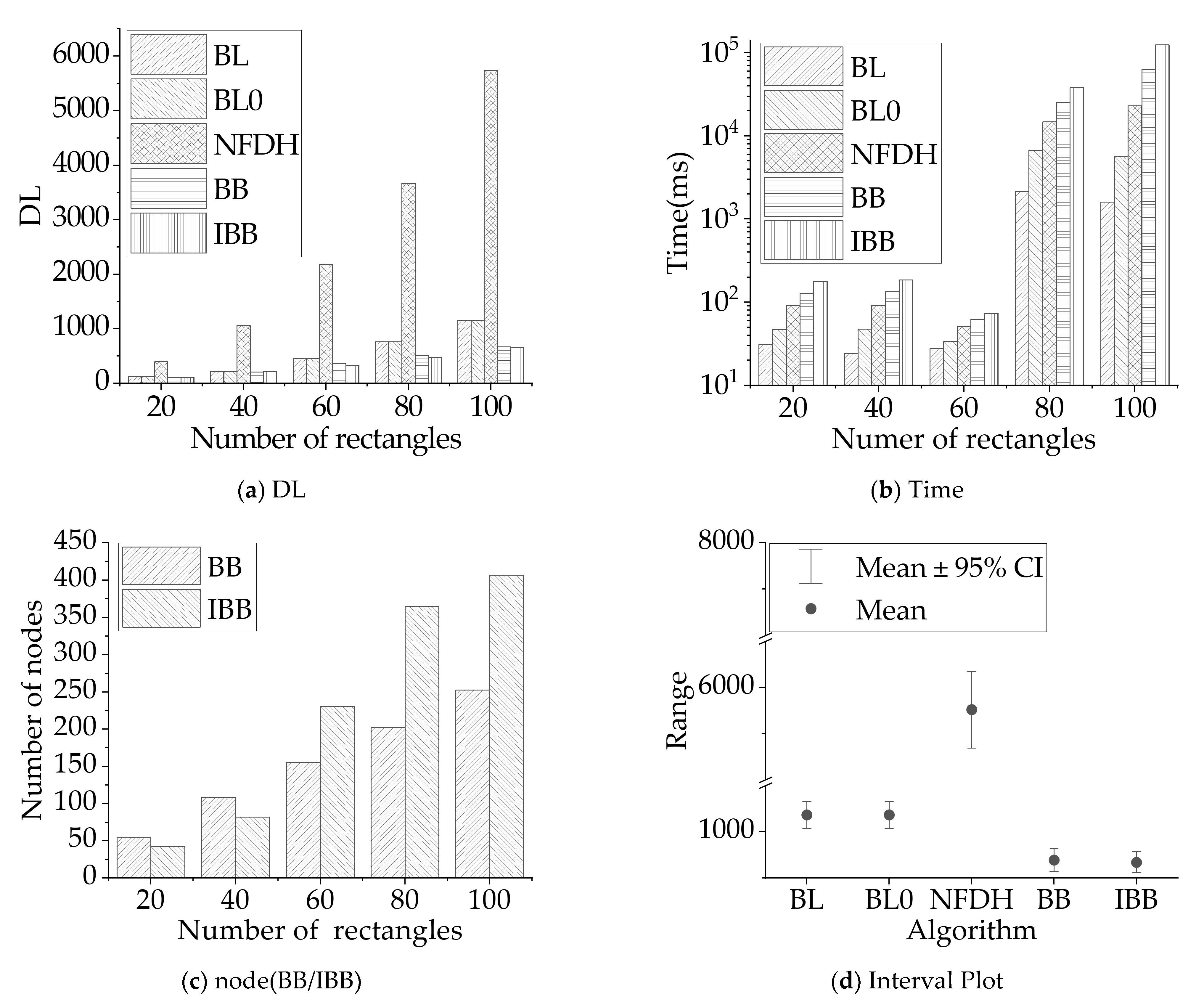
In Equations (25)–(28), N is the number of rectangles, N = {20,40,60,80,100}, and DLj is the total delay in the j-th rectangle According to Equation (14), we can determine the relaxation upper bound DLUB of the problem, which is the possible maximum area sum of all rectangles, divided by the grouping constraint GHCk. Then, DLUB can be taken as the relative value to calculate the scores Smax, Savg, and Smin proportional to the delay. A smaller score indicates a smaller delay (DL) and better effectiveness of the algorithm. The success rate Rs is defined as the number of experiments (out of 100 experiments) in which the algorithm reaches the optimal value of all algorithms. If two or more algorithms reach the optimal value, they will be included. In addition, based on Equation (11) in the previous section, the maximum upper boundary of delay is approximately the area of the rectangle. Figure 8 shows the comparison of the BL/BL0/NFDH/BB/IBB algorithms.
The experimental conditions are the same as those described in this subsection. In the comparison of delays in Figure 8a, it is observed that BB and IBB have the lowest delay and the best effect, while NFDH has the worst effect. In all our other experiments, the effect of BFDH/FFDH was not as good as that of NFDH, so the data for these experiments are not shown. Figure 8b shows a comparison of the calculation times. It is observed that IBB has the longest calculation time, which is even longer by several orders of magnitude. Therefore, we adopt the logarithmic Y coordinate system, and the order of calculation time is TIBB > TBB > TBL ≈ TBL0 > TNFDH. Figure 8c shows the comparison of search nodes between BB and IBB. It is observed that the number of search nodes of IBB exceeds 60 when the total number of rectangles is greater than 60, that is, the number of groups g > 6 will exceed BB and grow rapidly. Figure 8d shows the 95% delay spacing diagram. The NDFH algorithm is the most divergent in solving, followed by BL and BL0. BB and IBB are the most concentrated, and their average values are the smallest.
Table 6 compares the performance of the algorithms for the improved grouping constraint test instances. From the point of view of the optimal number of Rs, BB and IBB are better than BL0. The branch-and-bound method can search more space so that the solving effectiveness is better for BB and IBB than for BL0. Moreover, since NFDH, BFDH, and FFDH are not as effective as BL0, they are not listed in the results. BB outperforms IBB when the number of groups g is less than 6, but IBB performs better when the number of groups g is greater than 6 because IBB uses delay as the judgement basis for controlling the equivalence pruning. When the number of groups g is large, the advantage is clear. In addition, BB is inferior to IBB when g > 6, except at T3. The Rs of BB rises and the Rs of IBB declines in T4.
It remains to be studied whether increasing the number of groups g can make the optimal times of BB equal to or even surpass those of IBB. In Rs, the number of groups g > 6, and the IBB advantage is more pronounced, achieving a maximum improvement of 25% relative to the BB algorithm (Test T5, 80 rectangles).
In Smin/avg/Smax, the values of C2, C4, and C6 are larger than C1, C3, and C5 because a larger H/Lp of the problem corresponds to a smaller delay. For larger H, more space in the problem can be scheduled, and a smaller Smin/Savg/Smax is obtained. At the same time, it is also observed that in C1, C3, and C5, the Smin of IBB is slightly better than that of BB, but the IBB on Smax is partially worse than that of BB, indicating that under the condition of LpH, the solution of IBB is more divergent than that of BB. In T1~T4, Smin can be optimized for T1/T2/T4, while T3 cannot be optimized. In Smin/Savg/Smax, BB and IBB have little difference in solving ability, IBB is relatively divergent, and IBB’s optimal value is approximately 6% higher than that of BB (Test T4 80).

4.3. Performance with Lag Factor

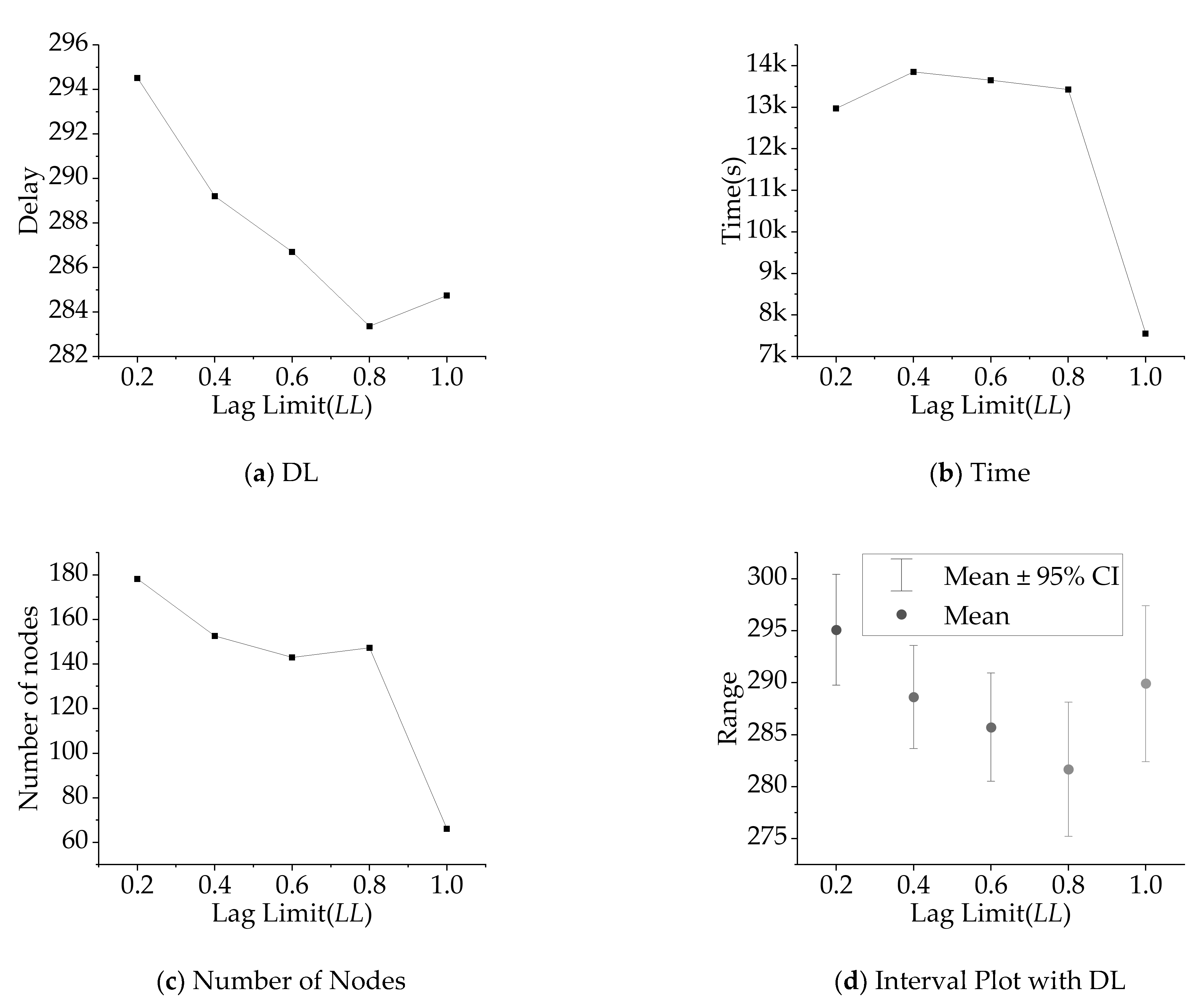
This subsection mainly studies the influence of the change in the lag limit (LL) on the algorithm. LSLk = kLr is set in the experiment. Lr is the upper limit of the generation length of test Class 1. The lag limit LL ∈ {0.2, 0.4, 0.6, 0.8, 1.0} is set. To save experimental time, the number of groups g = 8, the number of rectangles mk = 5 in each group, and the other conditions are the same as in this section. Figure 9 shows the influence of LL on the delay/time/number of search nodes, and Figure 9a shows the relationship between the delay and LL.
The delay decreases with increasing LL, reaching a minimum when LL = 0.8, and then rising slightly. Figure 9b shows the relationship between the calculation time and LL. The calculation time is relatively stable from LL = 0.2 to 0.8 and decreases rapidly when LL = 1.0. Figure 9c shows the relationship between the number of search nodes and LL. The number of search nodes decreases slowly with increasing LL and decreases rapidly after 0.8. Figure 9d shows the 95% confidence interval diagram. It is observed that the overall confidence interval has roughly the same length, but the average value decreases with the increase in LL, reaching the lowest value at 0.8 and then rising at 1.0. We also studied grouping constraints and delay, but the results were random, and there was no specific experimental conclusion.

4.4. Global Sensitivity Analysis

In this section, we perform a global sensitivity analysis (GSA) on the BB-RIA-LPO algorithm [26]. The analysis program used is provided by Flavio, which generates a Sobol quasi random set and Fourier amplitude sensitivity test (FAST) analysis. The test parameters are the lag limit (LL), number of groups (g), number of each group (mk), and the maximum range of width and height (Lp). Their parameter ranges are [0.6,1], [2,10], [10,20] and [2,8], respectively.
Table 7 shows the first-order global sensitivity coefficients of the FAST algorithm. It can be seen from the table that the number of groups (g) and the number of each group (mk) are relatively large for both the uniform random distribution and the Sobol quasi random set, which indicates that they have a great influence on the BB-RIA-LPO algorithm and confirms our previous discussion about group g > 6.

5. Rural Portfolio Credit Case

This section is a case simulated according to the actual “whole village credit” project: Under the background of implementing the “rural revitalization” policy, Bank H conducts the whole village credit business for Village L, with a total amount of 600 million yuan; credit is divided into organizations and villagers’ individuals. Organization loans are usually used for production investment or project construction, so there is a large loan amount, a long loan term, and a low requirement for the latest loan obtaining time. However, villagers’ individual loans are usually used for personal consumption and personal business. The use of funds is characterized by small loan amounts and short loan terms, so they hope to obtain loans in a short time. Because of the large number, in this example, for the convenience of demonstration, multiple personal consumption credits and personal business loans are combined, their amounts are summed, their terms are set as their average values, and the total amount is calculated as a whole for scheduling. Table 8 provides detailed information on the case.
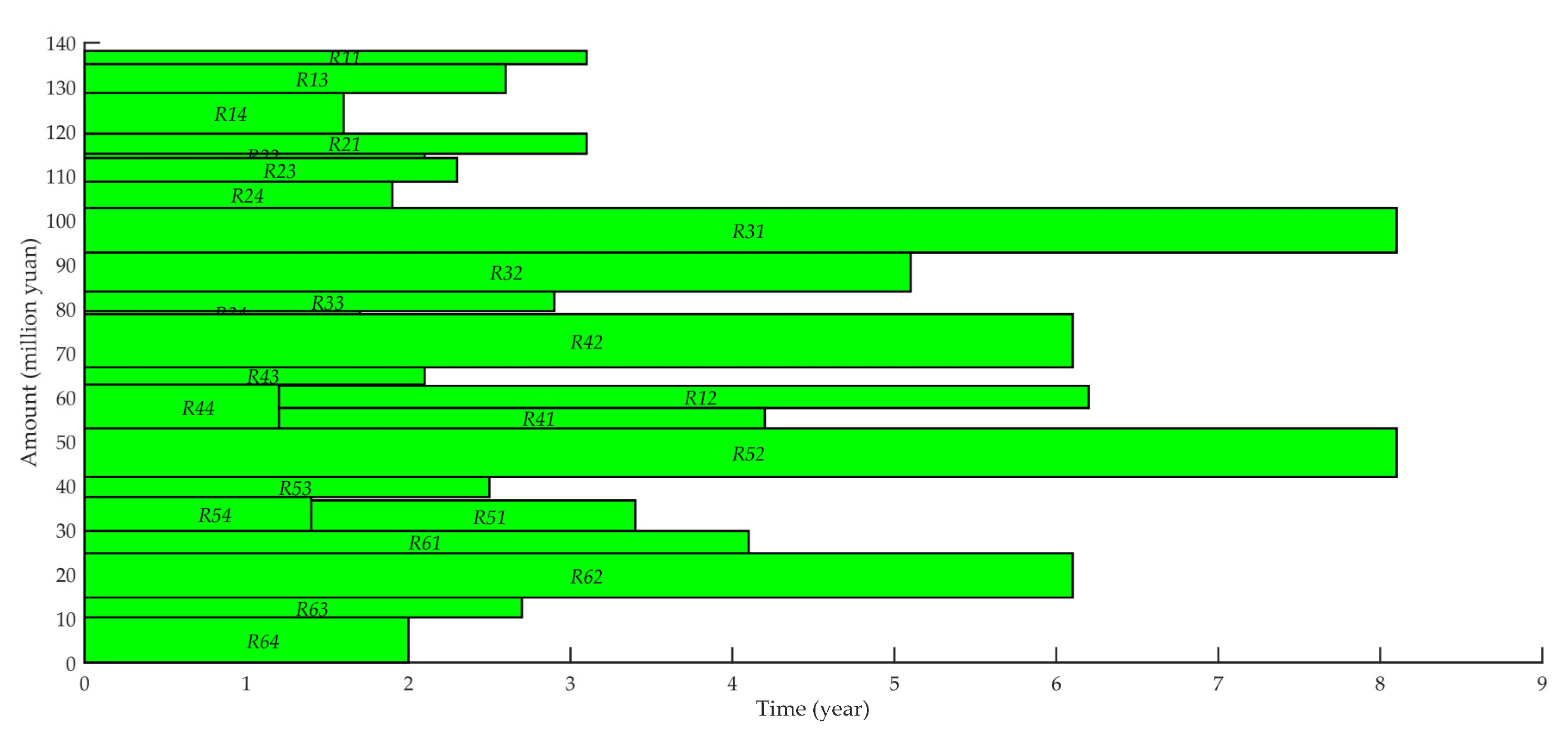
Figure 10 shows the Gantt chart of case scheduling. The mark Rki indicates the loan of the k-th village and the i-th item. All villagers’ loans have been dispatched, among which R12, R41, and R51, the villagers who received loans later, received loans for 1.2, 1.2, and 1.4 years. This is because the total amount of loan demand of the fourth and fifth villagers exceeds the credit amount of the village, so among them, the loan amount is large, and R41 and R51 with a long loan term will be delayed. For this case, the BL, BL0, and BB-RIA-LPO algorithms generate total delays of 10.7, 4.4, and 3.8 years, respectively. The new algorithm reduces the total delay by 15.79%.

6. Conclusions

In this paper, we study the solving algorithm of the portfolio credit-granting problem in the field of management. First, the portfolio credit granting problem in the field of system management is abstracted into the combinatorial (grouping) constraint two-dimensional packing delay optimization problem. Second, a mathematical model of two-dimensional packing delay optimization based on combinatorial constraints, that is, 2SPGDP, is established, and its upper bounds, lower bounds, and delays are studied. Third, BB-RIA, ISS, and LPO were used to solve the two-dimensional packing delay optimization problem.
Numerical experiments show that the method can solve the classical test instances correctly. In the two-dimensional packing problem, the improved method has better solution quality and success rate than the bottom-left algorithm (BL) when the number of groups is greater than 6. Compared with the classical branch and bound algorithm, the maximum success rate can be improved by 6–25%, and the total delay can be reduced by 6%. The lag limit of the improved algorithm can obtain the best solution quality at LL = 0.8. In the case of rural portfolio credit, the algorithm reduces the delay by 15.79%.
This study still has some limitations and needs further improvement. In terms of the algorithm, the relationship between the lag factor and grouping latest start length (LSL) setting has not been clearly studied. The algorithm with group number g < 6 and the solution time needs to be shortened. Second, from the actual problem of rural portfolio credit, a more rigorous risk mechanism needs to be added, and larger examples need to be verified.
In brief, the 2SPGDP model proposed in this paper can be used as a reference for the problem of combination constraint and delay optimization. The BB-RIA-LPO algorithm can reduce the delay and obtain a better solution. The algorithm is applied to the rural portfolio credit-scheduling problem to improve efficiency and better schedule preferential loans to villagers through grouping constraints. As rural loans are unsecured preferential loans with the attribute of public service, it is one way to strengthen the risk mitigation of rural commercial banks to adopt whole village credit and decentralized management, which is conducive to rural revitalization.

Author Contributions

Conceptualization, methodology, software, validation, formal analysis, investigation, resources, data curation, writing—original draft preparation, writing—review and editing, H.H.; writing—review and editing, visualization, supervision, project administration, Y.L. All authors have read and agreed to the published version of the manuscript.

Funding

This work is supported by the National Natural Science Foundation of China under Grant 62176102.

Institutional Review Board Statement

Not applicable.

Informed Consent Statement

Not applicable.

Data Availability Statement

The data were obtained from the European Operations Research Institute.

Conflicts of Interest

The author declares no conflict of interest.

References

  1. Chen, X.X.; Zheng, H.R. Research on Rural Inclusive Financial Credit Service from the Perspective of Satisfaction-Take Fujian sample of inclusive financial reform pilot area as an example. Financ. Theory Pract. 2022, 9, 69–80. [Google Scholar]
  2. Wang, Q. Research on the Optimization of the Whole Village Credit Business of CC Rural Commercial Bank. Master’s Thesis, Jilin University, Changchun, China, 2022. [Google Scholar] [CrossRef]
  3. Li, N. Study o the Farmer Loan Management Strategy of “Whole Village Credit” in W Branch. Master’s Thesis, Dalian University of Technology, Dalian, China, 2021. [Google Scholar] [CrossRef]
  4. Gao, L. Design of Credit Scheme for Rural Whole Village of Huanghe Bank. Master’s Thesis, Xi’an University of Technology, Xi’an, China, 2021. [Google Scholar] [CrossRef]
  5. Chen, W. Research on the Whole Village Credit Granting of Small Loans to Farmers in WH Rural Creit Union. Master’s Thesis, Zhengzhou University, Zhengzhou, China, 2021. [Google Scholar] [CrossRef]
  6. Liu, Y. Research on Problems and Countermeasures of JD Rural Commercial Bank’s “Whole Village Credit”. Master’s Thesis, Yangzhou University, Yangzhou, China, 2019. [Google Scholar] [CrossRef]
  7. Liu, M.; Tong, X.; Dai, Y. Recent developments in algorithms for packing problem. Math. Num. Sinica 2016, 38, 257–280. [Google Scholar]
  8. Cid-Garcia, N.M.; Rios-Solis, Y.A. Exact solutions for the 2d-strip packing problem using the positions and covering methodology. PLoS ONE 2021, 16, e0245267. [Google Scholar] [CrossRef] [PubMed]
  9. Qi, X.Y.; Zheng, Q.X.; Li, M.; Guo, T.J. The Model with Left Bottom Corner Coordinates for 2D Rectangular Strip Packing Problem. In Proceedings of the 2017 International Conference on Wireless Communications, Networking and Applications, Shenzhen, China, 20–22 October 2017; pp. 172–176. [Google Scholar]
  10. Souza Queiroz, L.R.D.; Andretta, M. A branch-and-cut algorithm for the irregular strip packing problem with uncertain demands. Int. Trans. Oper. Res. 2022, 29, 3486–3513. [Google Scholar] [CrossRef]
  11. Oviedo-Salas, E.; Terán-Villanueva, J.D.; Ibarra-Martínez, S.; Santiago-Pineda, A.; Ponce-Flores, M.P.; Laria-Menchaca, J.; Castán-Rocha, J.A.; Treviño-Berrones, M.G. GRASP Optimization for the Strip Packing Problem with Flags, Waste Functions, and an Improved Restricted Candidate List. Appl. Sci. 2022, 12, 1965. [Google Scholar] [CrossRef]
  12. Wei, L.; Hu, Q.; Leung, S.C.; Zhang, N. An improved skyline based heuristic for the 2D strip packing problem and its efficient implementation. Comput. Oper. Res. 2017, 80, 113–127. [Google Scholar] [CrossRef]
  13. Chen, Z.; Chen, J.L. An Effective Corner Increment-Based Algorithm for the Two-Dimensional Strip Packing Problem. IEEE Access 2018, 6, 72906–72924. [Google Scholar] [CrossRef]
  14. Chen, M.; Li, K.; Zhang, D.; Zheng, L.; Fu, X. Hierarchical Search-Embedded Hybrid Heuristic Algorithm for Two-Dimensional Strip Packing Problem. IEEE Access 2019, 7, 179086–179103. [Google Scholar] [CrossRef]
  15. Li, Y.-B.; Sang, H.-B.; Xiong, X.; Li, Y.-R. An Improved Adaptive Genetic Algorithm for Two-Dimensional Rectangular Packing Problem. Appl. Sci. 2021, 11, 413. [Google Scholar] [CrossRef]
  16. Mondal, S.; Tsourdos, A. Two-Dimensional Quantum Genetic Algorithm: Application to Task Allocation Problem. Sensors 2021, 21, 1251. [Google Scholar] [CrossRef] [PubMed]
  17. Neuenfeldt Júnior, A.; Francescatto, M.; Stieler, G.; Disconzi, D. A Multi-label Transformation Framework for the Rectangular 2D Strip-Packing Problem. Manag. Prod. Eng. Rev. 2021, 14, 27–37. [Google Scholar]
  18. Zheng, S.; Yang, Z.; He, Z.; Wang, N.; Chu, C.; Yu, H. Hybrid simulated annealing and reduced variable neighbourhood search for an aircraft scheduling and parking problem. Int. J. Prod. Res. 2019, 58, 2626–2646. [Google Scholar] [CrossRef]
  19. Vega-Mejia, C.A.; Montoya-Torres, J.R.; Islam, S.M.N. Consideration of triple bottom line objectives for sustainability in the optimization of vehicle routing and loading operations: A systematic literature review. Ann. Oper. Res. 2019, 273, 311–375. [Google Scholar] [CrossRef]
  20. Júnior, A.N.; Silva, E.; Francescatto, M.; Rosa, C.B.; Siluk, J. The rectangular two-dimensional strip packing problem real-life practical constraints: A bibliometric overview. Comput. Oper. Res. 2022, 137, 105521. [Google Scholar] [CrossRef]
  21. Parker, R.G. Deterministic Scheduling Theory, 1st ed.; Chapman & Hall: Boca Raton, FL, USA, 1996; pp. 25–35. [Google Scholar]
  22. Scheithauer, G. Introduction to Cutting and Packing Optimization- Problems, Modeling Approaches, Solution Methods, 1st ed.; Springer: Basel, Switzerland, 2018; pp. 183–225. [Google Scholar]
  23. Test Problems for 2D Rectangular Strip Packing: Benchmark Problems in Literature, the Association of European Operational Research Societies. Available online: https://www.euro-online.org/websites/esicup/data-sets/#1535972088188-55fb7640-4228 (accessed on 1 October 2021).
  24. Berkey, J.O.; Wang, P.Y. Two dimensional finite bin packing algorithms. J. Oper. Res. Soc. 1987, 38, 423–429. [Google Scholar] [CrossRef]
  25. Martello, S.; Vigo, D. Exact solution of the two-dimensional finite bin packing problem. Manag. Sci. 1998, 44, 388–399. [Google Scholar] [CrossRef]
  26. Cannavo, F. Sensitivity analysis for volcanic source modeling quality assessment and model selection. Comput. Geosci. 2012, 44, 52–59. [Google Scholar] [CrossRef]
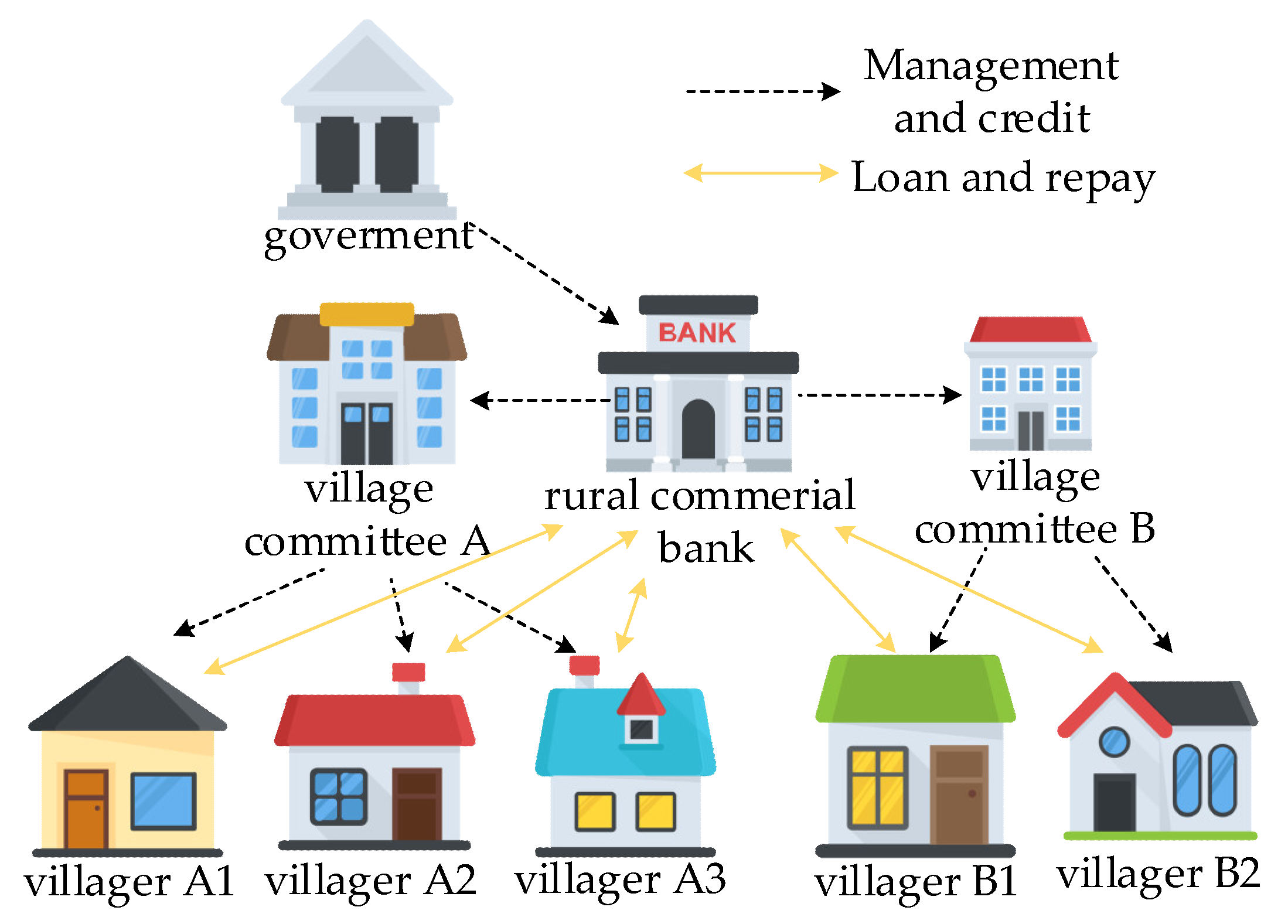
Figure 1. Rural credit relationship.
Systems 10 00193 g001
Figure 2. Simple example of 2SPGDP scheduling.
Systems 10 00193 g002
Figure 3. Example of calculating the delay time score.
Systems 10 00193 g003
Figure 4. Deep search reverse spanning tree (DSRST).
Systems 10 00193 g004
Figure 5. Skyline method and interpolation method: (a) Skyline method; (b) insert method.
Systems 10 00193 g005
Figure 6. Non-lag and lags. (a) Non-lag; (b) lag.
Systems 10 00193 g006
Figure 7. Flowchart of the branch-and-bound reverse-order insert algorithm with the lag pruning operator(BB-RIA-LPO).
Systems 10 00193 g007
Figure 8. Comparison of BL/BL0/NFDH/BB/IBB algorithms (Test C1).
Systems 10 00193 g008
Figure 9. Influence of delay factors on the delay/time/number of the search nodes.
Systems 10 00193 g009
Figure 10. Gantt chart of case scheduling.
Systems 10 00193 g010
Table 1. Symbol and parameter description and scheduling problem meanings.
SymbolDescriptionMeaning in Rural Portfolio Credit Scheduling Problem
GkThe group k (k = 1, 2, …, g, k ∈ N+)Group k of portfolio credit project
RkiThe i-th rectangle of Group k(i = 1, …, mk, iN+)The i-th item of Group k
hkiHeight of the i-th rectangle of Group kLoan amount of the i-th item
lkiLength of the i-th rectangle of Group kLoan term of the i-th item
LSLkiThe latest start length of the i-th rectangle of Group kLatest loan obtaining time for the i-th item of Group k
GHCkHeight constraint of Group kThe total credit of Group k
SLkiThe start length of the i-th rectangle in Group kScheduling start time for the i-th item of Group k
ELkiThe end length of the i-th rectangle in Group kScheduling end time for the i-th item of Group k
DLkiThe scheduling delay length of the i-th rectangle in Group kScheduling delay time for the i-th item of Group k
Table 2. Simple example parameters.
Rural Portfolio Credit2SPGDP
villageGroup k11122
loan itemRectangle Rki12312
loan amount(million yuan)Height hki22121
loan term(year)Length lki21222
latest loan obtaining time (year)Latest start length LSLk0.20.4
village credit limit(million yuan)Height Constraint GHLk43
Table 3. Branch and bound reverse order insert algorithm with lag pruning operator (BB-RIA-LPO).
Initialization, the loop begin, ks = 0, count = 0.
If the current strip box placement point queue is empty, then find all placement points and put them in the placement point queue.
Have all placement points in placement point queue been scheduled? If yes, go to ④, backtracking; otherwise, set the current placement point as the scheduling point and go to ⑦.
Go back to the previous layer, ks = ks − 1.
Check if ks = 0, count the number of times that ks is assigned to 0 and record it in the variable count.
If the count < = |R|, then count = count + 1, and go to ②, the next loop; otherwise, stop and end the algorithm.
Whether to arrange all rectangles depends on whether the rectangle queue is empty. If yes, go to ⑧; otherwise, go to ② for the next loop.
Will the lag operator be set? If yes, check the lag. Otherwise, switch to ⑨.
Pre-dispatch and check over the limit; if the height of the strip box is exceeded, go to ② for the next loop.
Are the group constraints met? If not, go to ② for the next loop.
Is equivalence and dominance satisfied? If not, go to ② for the next loop.
Regarding dispatching rectangles, calculating object values Lopt and recording paths, is it at the bottom? If yes, go back to ks = ks − 1 and go to ② for the next loop; otherwise, search down, ks = ks + 1.
Table 4. Performance comparison of classical test instances.
TestBLNFDHBBIBB
LoptTimeLoptTimeLoptTimeLoptTime
J129362214191873318615
J224461813221680221640
D1606052680521701521680
D2544047154585545792
D31388201311714323801302330
D4233462451523619702231920
Kendell1406621030140956140934
Table 5. Grouping constraint test settings.
TestDenoteDescription
Class 1C1H = 10, hj and lj at random in [1,10]
Class 2C2H = 30, hj and lj at random in [1,10]
Class 3C3H = 40, hj and lj at random in [1,35]
Class 4C4H = 100, hj and lj at random in [1,35]
Class 5C5H = 100, hj and lj at random in [1,100]
Class 6C6H = 300, hj and lj at random in [1,100]
Type 1T1hj at random in [2/3 H, H]; lj at random in [1, 1/2 H]
Type 2T2hj at random in [1, 1/2 H]; lj at random in [2/3 H, H]
Type 3T3hj at random in [1/2 H, H]; lj at random in [1/2 H, H]
Type 4T4hj at random in [1, 1/2 H]; lj at random in [1, 1/2 H]
Table 6. Performance comparison of algorithms for improved grouping constraint test instances.
Test RSSminSavgSmax
BL0BBIBBBBIBBBBIBBBBIBB
C1201100887715162633
40010082121231325656
6006185262551517676
80071753939666796103
1000718249498484126126
C22026776611551313
4058423611441212
6018516911441212
8016587111441212
1009587811541413
C320399873311112727
400100768824254646
6006481161536355959
8007180242448487676
10007675353560609091
C42037635500441313
404654430044910
6016547000551312
8015616911551619
1003728011661614
C5201097865525254142
40010084111125254849
6005588201941416664
8006379282752527982
100070783535676798106
C62039645800441212
4068322700441212
602949600044119
8029525211441517
10014636700551322
T1201097865525254142
4001009025255859103103
600588450509392138147
80059817777122122165163
10005883109108159159206238
T220594713321223939
4009985252551517575
600647838337877112112
80069846055107106158158
100070887777136135195195
T32049981131334355555
401998145457374105105
60067628582116117157163
8006868118118154154187187
10006475157157192192229230
T420398830011113939
400100722227289999
6006687664342115115
800768616105858118118
1000768018187978158158
Table 7. Performance comparison of algorithms for improved grouping constraint test instances.
LLgmkLp
Uniform0.00390.22320.02400.4028
Sobol0.00590.22190.02140.3987
Table 8. Performance comparison of algorithms for improved grouping constraint test instances.
GkiProjectAmountTotal Loan
Amount
Loan
Term
Latest
Obtaining
Time
Village
Credit
11Automatic irrigation equipment for planting13030.25300
12Treatment of pig breeding wastes15050.25
13Personal business loans33652.50.1
14Personal consumption loans142921.50.1
21Meat intensive processing production line14530.25300
22Egg incubator equipment13220.25
23Personal business loans26532.20.1
24Personal consumption loans123591.80.1
31Supporting facilities of “Hot Spring Village” featured health care center110080.25300
32Greenhouse planting facilities18850.25
33Personal business loans18442.80.1
34Personal consumption loans102711.60.1
41Attached aquaculture equipment for abalone aquaculture14630.25300
42Agricultural Products Wholesale Center Project112060.25
43Personal business loans163920.1
44Personal consumption loans99991.10.1
51Land fertility improvement project of fruit and vegetable base16920.25300
52Low temperature finished grain storage construction project111080.25
53Personal business loans18452.40.1
54Personal consumption loans102771.30.1
61Irrigation and drainage pump station renovation project15040.25300
62Photovoltaic power generation energy construction project110060.25
63Personal business loans16452.60.1
64Personal consumption loans9910201.90.1
Publisher’s Note: MDPI stays neutral with regard to jurisdictional claims in published maps and institutional affiliations.