Distance-Based Decision Making, Consensus Building, and Preference Aggregation Systems: A Note on the Scale Constraints

Abstract

Distance metrics and their extensions are widely accepted tools in supporting distance-based decision making, consensus building, and preference aggregation systems. For several models of this nature, it may be necessary to elucidate the problem output in the original input domain. When a particular parameter of interest is desired to be produced in this original domain, i.e., the scale, the decision makers simply resort to constraints that function in parallel with this goal. However, there exist some cases where such a membership is guaranteed by the mathematical properties of the distance metric utilized. In this paper, we argue that the scale constraints utilized in this manner under the distance-metric optimization framework are, in some cases, completely redundant. We provide necessary mathematical proofs and illustrate our arguments through an abstract physical system, examples, a case study, and a brief computational experiment.

1. Introduction and Related Literature

Decision making is concerned with finding the best alternatives from a finite choice set with regard to their total performances over several relevant criteria. When there is a single individual to make the decision or a committee chooses to act as a solitary decision-making unit, a single decision maker setting emerges [1,2,3,4]. Otherwise, each member of the committee delivers his/her preferences separately and such assessments have to be aggregated into a group decision calling for a group consensus or a group decision-making scenario [5,6,7,8,9,10]. The preference information, so crucial to reaching a valid decision, is highly dependent on the decision situation and the decision maker’s or the committee’s knowledge, experience, perception, and comprehension of the situation. The theory of decision making is well able to support a variety of preference information categories. Such information can be provided in cardinal [11,12], ordinal [13,14], linguistic [5,15], fuzzy [16,17], interval [18,19,20], multi-granular [21,22], multiplicative [23,24], pair-wise [25,26], and incomplete [27,28] arrangements. The relative importance of the criteria has to be amassed with this information in some way, to obtain the total performances of the decision alternatives. Usually, it is stated as suitable criteria weights, which can either be pre-specified [14] due to some previous experience, separately obtained by some method [26], or extracted from partial information [29].

Various systems were studied and practiced in the past to synthesize the above information. Of particular interest to us in this paper are those relying on distance metrics to support decision making, consensus building, and preference aggregation, namely the distance-based systems (DBS). In mathematics, a metric is a function that assigns a non-negative distance between the elements of a space. A subset of these functions, the infamous ${\ell }_p$ (or, alternatively, the order p Minkowski) metrics, is extensively used in DBS due to its desirable properties, such as non-negativity, symmetry, and triangle inequality. For detailed information on ${\ell }_p$ metrics, we refer the reader to the body of work [30,31,32].

To illustrate, let $\mathcal{V}$ be a vector space and $v,u\in \mathcal{V}$ be two vectors of order $n$, such that $v=\left(v_1, v_2,\dots , v_n\right)$ and $u=\left(u_1, u_2,\dots , u_n\right)$. This subset of distance functions is characterized by a single-order parameter $p$ and assumes the general form:

$$d\left(\mathit{v}, \mathit{u}\right)\equiv {\ell }_p\left(\mathit{v}, \mathit{u}\right)={\left({\displaystyle \sum }_{i=1}^n{\left|v_i-u_i\right|}^p\right)}^{\frac{1}{p}}, 1\le p\le \infty ,$$

(1)

where $d\left(\mathit{v}, \mathit{u}\right)$ is the distance between vectors $\mathit{v}$ and $\mathit{u}$, and $i$ is an index. Due to the order parameter $p$, general ${\ell }_p$ Equation (1) provides a useful family of metrics to measure the distance where applicable, depending on the specific problem domain and characteristics.

A collection of methodologies hinge on this family of metrics for the minimization of distance to some form of a pre-specified and desired configuration, sometimes called the ideal or the utopia. Some typical examples are goal programming [33], reference point methods [34], compromise programming [35], and composite programming [36]. Other non-standard procedures are tailored to employ such metrics in some stage of their execution. Our review of the subject literature revealed that not only this family of metrics but also their extensions and special definitions are widely used as distance measures to support DBS. For the convenience of the reader, we summarized our detailed overview of these studies in

Table 1. Summary of subject literature.

Source	Domain	Distance Notion	Features	Illustration
[47]	Group consensus	General ${\ell }_p$ metric	Goal programming	Voting
[14]	Single decision maker	Distance between pre-orders	Order theory	Numerical example
[44]	Group consensus	Separation distance	Compromise programming	Conservation planning
[41]	Single decision maker	Profile distance	Utility theory	ERP software selection
[13]	Screening, group consensus	Distance between pre-orders	Order theory	Numerical example
[5]	Group consensus	Fuzzy distance	Clustering	Software selection
[10]	Group consensus	Euclidean	Decision support systems	Facility planning
[25]	Group consensus	General ${\ell }_p$ metric	Goal programming	Numerical examples
[48]	Single decision maker	Euclidean	Decision balls	Numerical example
[37]	Single decision maker	Rectilinear, Chebyshev	Fuzzy multi-objective program	Numerical example
[11]	Screening	Case-based distance	Case-based reasoning	Water resources planning
[9]	Group consensus	Rectilinear	Assignment model	Evaluation of IT security
[42]	Screening	Rectilinear	Feature extraction	Classification of signals
[1]	Single decision maker	Euclidean, Mahalanobis	Rule-based reasoning	Decision support system
[17]	Group consensus	Euclidean	Intuitionistic fuzzy sets	Merger strategy evaluation
[38]	Group consensus	General ${\ell }_p$ metric	Goal programming	Performance appraisal
[22]	Group consensus	General ${\ell }_p$ metric	Fuzzy sets	Recruiting
[15]	Group consensus	Rectilinear	Fuzzy sets	Project selection
[8]	Group consensus	Rectilinear, Euclidean	Consistency indices	Numerical example
[40]	Group consensus	Fuzzy distance	Fuzzy sets	Performance evaluation
[45]	Group consensus	Similarity measure	Intuitionistic fuzzy sets	Evaluation of air quality
[12]	Group consensus	Squared Euclidean	Lagrangian function	Emergency decision support
[49]	Group consensus	Similarity measure	Fuzzy sets	Site selection
[46]	Group consensus	Profile distance	Bisection algorithm	Computational experiment
[50]	Group consensus	Rectilinear	Induced aggregation operators	Investment planning
[51]	Group consensus	Rectilinear	Intuitionistic fuzzy sets	Investment planning
[7]	Group consensus	Rectilinear	Linear orders	Numerical example
[27]	Group consensus	Rectilinear	Logarithmic goal programming	Numerical example
[28]	Single decision maker	Euclidean	Nonlinear programming	Investment planning
[52]	Group consensus	General ${\ell }_p$ metric	Hesitant fuzzy sets	Energy policy assessment
[43]	Single decision maker	Rectilinear	Induced aggregation operators	Football player selection
[53]	Single decision maker	Affinity distance	Co-evolutionary algorithm	Garment manufacturing
[39]	Group consensus	Euclidean	Interval-valued fuzzy sets	Manager selection
[2]	Single decision maker	General ${\ell }_p$ metric	Quadratic optimization	Credit risk analysis
[4]	Single decision maker	Euclidean	Data mining	Incident risk analysis
[3]	Single decision maker	Dissimilarity measure	Belief functions	Numerical examples
[6]	Group consensus	Signed distance	Interval-valued fuzzy sets	Supplier selection
[54]	Single decision maker	Euclidean	Lagrangian function	Machine selection
[55]	Group consensus	Fuzzy max and min distance	Induced aggregation operators	Strategy development
[56]	Group consensus	Rectilinear	Goal programming	Investment planning
[57]	Group consensus	Hausdorff	Sensitivity analysis	Forecasting method selection
[58]	Single decision maker	General ${\ell }_p$ metric	Multi-objective programming	Project selection
[59]	Single decision maker	General ${\ell }_p$ metric	Goal programming	Indicator ranking
[60]	Single decision maker	Similarity measure	Hesitant fuzzy sets	ERP system selection
[61]	Single decision maker	Belief interval distance	Belief functions	Numerical example
[62]	Group consensus	Hausdorff	Hesitant fuzzy sets	Investment planning
[63]	Group consensus	Euclidean and Hausdorff	Type-2 fuzzy sets	Numerical example
[64]	Single decision maker	Z-number distance	Choquet Integral	Inquiry selection
[65]	Single decision maker	Euclidean and Hausdorff	Set pair analysis	Case study
[66]	Single decision maker	Fuzzy distance	Nonlinear optimization	Disaster decision making
[67]	Group consensus	Fuzzy similarity measure	Type 1 and 2 fuzzy sets	Illustrative examples
[68]	Single decision maker	Distance to target	Sustainability patterns	Assessment of indicators
[69]	Group consensus	Euclidean	Preference relations	Project selection
[70]	Single decision maker	Similarity measure	Shannon entropy	Document identity identification
[71]	Single decision maker	Context-based distance	Intuitionistic fuzzy sets	Route decision making
[72]	Group consensus	Pair distance	Belief functions	Numerical example
[73]	Single decision maker	Divergence measure	Dempster-Schafer theory	Pattern classification
[74]	Single decision maker	Negation measure	Quantum information fusion	Pattern classification
[75]	Single decision maker	Belief Rényi divergence	Belief entropy	EEG data analysis
[76]	Single decision maker	Belief divergence measure	Dempster-Schafer theory	Pattern classification

. In order to disclose significant characteristics of each study, we organized four columns after the source information. The domain column is reserved for indicating in which setting, or for what purpose, the distance framework is used (i.e., in the single decision maker setting [37], in the group consensus setting [38], for screening the decision alternatives [11], etc.). The distance notion column shows which metric, or which specially defined form as a metric-based distance measure, is employed to support the method described in that paper (i.e., general ${\ell }_p$ [25], rectilinear [15], Euclidean [39], distance between pre-orders [13], fuzzy distance [40], signed distance [6], etc.). The features column lists which well-granted method, relevant concept, or theory is utilized or whose principles among these were engaged during implementation (i.e., the utility theory [41], feature extraction [42], case- and rule-based reasoning [1], Lagrangian function [12], induced aggregation operators [43], quadratic optimization [2], etc.). Finally, the illustration column is devoted to indicating the scheme preferred by the authors to verify their findings along with the case, or the system, where the corresponding study is piloted (i.e., the case study [44], numerical example [45], computational experiment [46], experimental study [42], etc.).

While the preference of a specific distance measure is usually intended for various goals, such as consensus, ranking, screening, consistency adjustment, etc., implementation of some form of the general ${\ell }_p$ metric or its custom modification is central to DBS. Hence, the principles of distance-metric optimization indeed apply to this group of procedures. In distance-metric optimization, sometimes a parameter of concern does not need to be necessarily constrained to have its final value fall within a target set. This is because such an association may be guaranteed by some gratifying mathematical property of the metric used. As will be clear later in this paper, what we have just noted is exactly the case in DBS.

In order to obtain the preference information from a decision maker or a committee, the typical practice in DBS is to utilize a common scale, including numbers or labels representing the preferences of the decision maker(s). When the final value of a parameter of interest needs to be expressed in this original domain, we impinge upon this parameter to occur within the limits prescribed by such a scale. These constraints are called the scale constraints in DBS.

In this paper, we argue for some cases in DBS that, due to the utilization of the family of metrics (1), the scale constraints that are put in practice to obtain the final values of parameters as elements of the original scale are actually not needed. Hence, it is interesting to observe that the scale constraints become redundant in practice. Through our discussion, we first introduce this idea to the reader on an abstract physical system, and then, we prove the redundancy result on some existing models. Finally, we illustrate our argument on some published examples, a case study, and a brief computational experiment.

On that account, our contribution is two-fold. First, due to the arguments of the paper, decision makers utilizing the distance-metric framework in objective functions are informed that they do not need the additional scale constraints to obtain the final values of the parameters of interest to be constrained within their initial scale. Second, based on the elimination of the scale constraints, it is suggested that they may not need to resort to optimization in solving such models. Moreover, the possible riddance of such insignificant constraints will lead to simpler problem representations.

We organized the remainder of this paper as follows. In Section 2, we discuss a mechanical apparatus which is an excellent abstraction of our entire discussion. Section 3 is reserved for the proof our argument mathematically. In Section 4, we test our outcomes on some examples and present the case study and the experiment. Subsequently, we come to an end with our conclusions in Section 5.

2. An Abstract Physical System

Consider a finite number of points located in a bounded two-dimensional region $\mathcal{R}$ and associate a nonnegative scalar with each point representing some form of weight assigned to it. Suppose that we measure the distances between the point locations using the Euclidean metric ${\ell }_2$. Furthermore, suppose that we aim to determine a new point in $\mathcal{R}$, say v, such that the sum of the weighted Euclidean distances from v to these points is minimal. This problem has a long history and is called the Weber, min-sum or 1-median problem (see [77] for a complete treatment of the problem and [78] for a connection to other location problems). In an industrial setting, each distinctive weight usually assumes the costs per unit distance of delivering some commodity from v to the respective point. In this scenario, the totality obtained by the summation of the resulting weighted Euclidean distances is a function representing the total transportation cost. The location of point v is the minimizer of this totality and is called the point of minimum aggregate travel, the Weber point, or simply the spatial median.

The above-stated problem is particularly important for our discussion in this paper. A surprisingly easy solution method for this problem is based on a mechanical device, as follows. Suppose we have a plane representing the two-dimensional region $\mathcal{R}$. First, we drill holes through this plane at the coordinates representing the point locations. Then, for each point, we bring out a string and a physical mass of the same magnitude as its specific weight. We tie the ends of the strings together to obtain a knot. Leaving the knot on one surface of the plane, we steer each string through a hole to its other surface. After that, we position the plane horizontally to stillness such that the free ends of the strings hang down from the holes. Finally, we attach the physical mass associated with each point to the string assigned to it. The apparatus we obtain by following these guidelines is called the Varignon frame. An illustration of a frame designed to find the spatial median of the four given points is provided in Figure 1a.

Now, suppose that the device we prepared is isolated from the drawbacks of a physical environment. For example, it is under the conditions in which the plane is frictionless, the holes are very small and also frictionless, the strings are very thin, such that their weights are almost ignored, etc. What happens in the case that we leave the masses to gravity and allow the knot to move liberally on the surface? It is easy to see that, due to the masses, each string will impose a force component on the knot and try to pull it towards its hole as much as possible. Eventually, the knot will move to a stable position and stop. This ultimate knot location is the anticipated spatial median of the given points.

To gain valuable insights from this solution, let us now construct the convex hull associated with these points on the surface. Figure 1b is a depiction of the surface where the convex hull, denoted here by $\mathcal{C}$, is shown with a shaded area. It is important for us at this point to observe that the spatial median cannot occur outside the convex hull. This is because there is no force component pulling the knot outside the convex hull. What then happens when a mass outweighs the sum of all the other masses? As there is no friction, the weight of this particular mass will pull the knot down its own hole. This is the most extreme case that can happen, where the optimal solution of the underlying Weber problem occurs exactly on one of the given points. To see it alternatively, recall the Weber problem under the industrial setting and observe that translating the knot location to any neighborhood of the hole is costly in this case.

To summarize, the optimal solution of the above Weber problem can only occur within a non-dominated subset of feasible solutions. Moreover, this set exactly sizes up to the convex hull of given points. While we aimed to generate a point v in $\mathcal{R}$ at the beginning, we came to see that its membership is guaranteed even in a more reserved set. It is clearly evident that we did not need a constraint to impose $v\in \mathcal{R}$, especially when we found out that $v\in \mathcal{C}$ was guaranteed.

3. Analysis

For our purposes, consider the following consensus-building problem.

Problem 1.

Given $n$ decision alternatives and $m$ committee members, each providing a judgment matrix $A^k=\left(a_{ij}^k\right)$ of order $n$, compute a consensus matrix $C=\left(c_{ij}\right)$ from the judgment set $\mathcal{A}=\left\{A^k :k=1,\dots ,m\right\}$ such that the collective error due to individual displacements $\left|c_{ij}-a_{ij}^k\right|$ between the consensus judgment and the personal judgments is as small as possible.

The above problem arises when the members of a committee settle upon acting as an individual decision-making unit. Hence, a consensus matrix representing the members’ aggregated preferences in the form of consensus judgments has to be computed. This problem is elaborated by the adoption of a metric-based approach to compute C that differs from $\mathcal{A}$ to the smallest possible extent under a pair-wise comparison scheme [25]. In this approach, the collective error originates from a series of displacements of each $c_{ij}$ from the corresponding m entries $a_{ij}^k$ arranged in the same position $\left(ij\right)$ of m pair-wise comparison matrices $A^k$, and it is measured with the employment of the general ${\ell }_p$ metric. Though we selected this particular DBS and some related examples to illustrate our arguments, one very important clarification is needed at this point. We clearly and vigorously stress that our aim is neither to criticize the valuable mathematical models presented nor to judge the usefulness of the results in [25]. Our only aim is to illustrate the argument that relates to scale constraints. These models are only selected because they are of very appropriate simplicity, which enhances the demonstration of our idea and the comprehension of the argument by the reader.

The optimization model associated with Problem 1 is as follows:

$$\left(M1\right) min f\left(C\right)={\left({\displaystyle \sum }_{k=1}^m{\displaystyle \sum }_{i=1}^n{\displaystyle \sum }_{\begin{array}{c}j=1\\ j\ne i\end{array}}^n{\left|c_{ij}-a_{ij}^k\right|}^p\right)}^{\frac{1}{p}}$$

(2)

subject to

$$0.111\le c_{ij}\le 9, i,j=1,\dots ,n, j\ne i.$$

(3)

It was suggested that the constraint set must satisfy some scale conditions to anchor the consensus judgments to the original scale domain. Hence, the constraints (3) were appended to establish those of Saaty’s pair-wise comparison scale (Saaty, 1980). This is an uncomplicated model and a good basis by which to illustrate the redundancy of scale constraints.

Consider a general-purpose pair-wise comparison scale $\mathcal{S}=\left(1/s,\dots ,1,\dots ,s\right),$ where $s>0$, and suppose that the personal judgments $a_{ij}^k$ are selected from $\mathcal{S}$ and arranged in $m$ pair-wise comparison matrices $A^k$. Thus, the scale constraints under $\mathcal{S}$ are of the form:

$$\frac{1}{s}\le c_{ij}\le s, i,j=1,\dots ,n, j\ne i.$$

(4)

To establish the redundancy result, first let $a_{ij}^k$ be arranged on the real line $\Re$ and consider the sets $A_{ij}=\left\{a_{ij}^k :k=1,\dots ,m\right\}$. We introduce the following definition.

Definition 1.

The linear hull $\mathcal{H}\left(A_{ij}\right)$ of the set $A_{ij}$ is the intersection of all real line segments containing $A_{ij}$.

On the real line, we simply have $\mathcal{H}\left(A_{ij}\right)=\left[a_{ij}^{-}, a_{ij}^{+}\right],$ where $a_{ij}^{-}=mi{n}_k\left\{a_{ij}^k : a_{ij}^k\in A_{ij}\right\}$ and $a_{ij}^{+}=ma{x}_k\left\{a_{ij}^k : a_{ij}^k\in A_{ij}\right\}$. For convenience, denote the elements of the unknown optimal consensus matrix $C^{\ast }$ by $c_{ij}^{\ast }$ and refer to this matrix as the optimal solution to Problem 1.

Theorem 1.

$\exists C^{\ast }$ where $c_{ij}^{\ast }\in \mathcal{H}\left(A_{ij}\right), \forall i,j;j\ne i.$

Proof of Theorem 1.

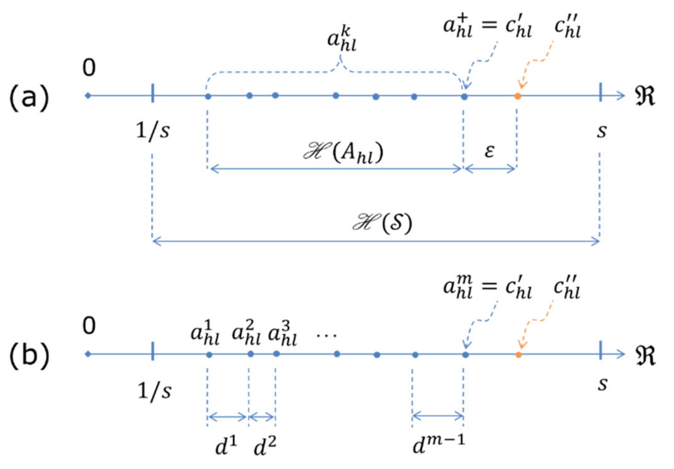
To prove Theorem 1 for $M1$, we create two solutions, $C^{\prime }$ and $C^{″}$, as follows. First, we isolate the entries $c_{hl}^{\prime }$ and $c_{hl}^{″}$ at the position $\left(hl\right)$ of both matrices. Then, we fill the matrices by picking an element from each set $A_{ij}$ and assigning it to the position $\left(ij\right)$ of both matrices. Hence, we have $c_{ij}^{\prime }=c_{ij}^{″} \forall i\ne h, \forall j\ne l,i$. Yet, for $c_{hl}^{\prime }$ we assign $c_{hl}^{\prime }=a_{hl}^{+}$. Then, since $c_{ij}^{\prime }\in A_{ij}\subset \mathcal{H}\left(A_{ij}\right)\subseteq \mathcal{H}\left(\mathcal{S}\right)$ and $c_{hl}^{\prime }\in A_{hl}\subset \mathcal{H}\left(A_{hl}\right)\subseteq \mathcal{H}\left(\mathcal{S}\right)$, clearly $C^{\prime }$ is a feasible solution satisfying $f\left(C^{\ast }\right)\le f\left(C^{\prime }\right)$. Now, suppose that we select $c_{hl}^{″}\in \mathcal{H}\left(\mathcal{S}\right)\backslash \mathcal{H}\left(A_{hl}\right)$, where $c_{hl}^{″}$ is arranged at a distance $\epsilon >0$ to the closest judgment term $c_{hl}^{\prime }=a_{hl}^{+}$, as shown in Figure 2a. Observe that only the displacements associated with $c_{ij}^{\prime }$ and the corresponding $m$ judgment terms $a_{ij}^k$ arranged in the same position $\left(ij\right)$ of the $m$ pair-wise comparison matrices are considered in the objective function $f\left(C^{\prime }\right)$. A similar argument is also true for $f\left(C^{″}\right)$. As $c_{ij}^{\prime }=c_{ij}^{″} \forall i\ne h, \forall j\ne l,i$; the difference between $f\left(C^{\prime }\right)$ and $f\left(C^{″}\right)$ is solely due to the terms ${\left|c_{hl}^{\prime }-a_{hl}^k\right|}^p$ and ${\left|c_{hl}^{″}-a_{hl}^k\right|}^p$. For convenience, we bring in the following term:

$$z\left(p\right)={\displaystyle \sum }_{\begin{array}{c}i=1\\ i\ne h\end{array}}^n{\displaystyle \sum }_{\begin{array}{c}j=1\\ j\ne l,i\end{array}}^n{\left|c_{ij}^{\prime }-a_{ij}^k\right|}^p={\displaystyle \sum }_{\begin{array}{c}i=1\\ i\ne h\end{array}}^n{\displaystyle \sum }_{\begin{array}{c}j=1\\ j\ne l,i\end{array}}^n{\left|c_{ij}^{″}-a_{ij}^k\right|}^p.$$

(5)

Note that the judgment terms $a_{hl}^k$ on the real line are in total order. Hence, without loss of generality, they can be re-indexed, say by $q$, leading to $a_{hl}^q$, as shown in Figure 2b. Denote the absolute displacement between each adjacent pair $\left\{a_{hl}^q, a_{hl}^{q+1}\right\}$ by $d^q$, where $d^q=a_{hl}^{q+1}-a_{hl}^q$. Then, in particular, the objective functions $f\left(C^{\prime }\right)$ and $f\left(C^{″}\right)$ are given by the following:

$$\begin{array}{c}f\left(C^{\prime }\right)=\left[z\left(p\right)+{\left(d^1+\dots +d^{m-1}\right)}^p+{\left(d^2+\dots +d^{m-1}\right)}^p\right.+\dots \hfill \\ \hfill {\left.\dots +{\left(d^{m-2}+d^{m-1}\right)}^p+{\left(d^{m-1}\right)}^p+0\right]}^{\frac{1}{p}}\end{array}$$

(6)

$$\begin{array}{c}f\left(C^{″}\right)=\left[z\left(p\right)+{\left(d^1+\dots +d^{m-1}+\epsilon \right)}^p+{\left(d^2+\dots +d^{m-1}+\epsilon \right)}^p+..\right.\hfill \\ \hfill {\left.\dots +{\left(d^{m-2}+d^{m-1}+\epsilon \right)}^p+{\left(d^{m-1}+\epsilon \right)}^p+{\epsilon }^p\right]}^{\frac{1}{p}}.\end{array}$$

(7)

As $d^q\ge 0$, $\epsilon >0$, and $p\ge 1$, a member-to-member comparison of the above objective functions shows that $f\left(C^{\prime }\right)<f\left(C^{″}\right)$. Therefore, we have $f\left(C^{\ast }\right)\le f\left(C^{\prime }\right)<f\left(C^{″}\right),$ which proves Theorem 1 for $M1$. □

Figure 2. Illustration of Theorem 1: (a) an arrangement; (b) re-indexing.

Figure 2. Illustration of Theorem 1: (a) an arrangement; (b) re-indexing.

Theorem 1 clearly shows that the optimal solution of $M1$ can only occur in a subset of feasible solutions where each entry $c_{ij}^{\ast }$ of the optimal solution is a member of the corresponding linear hull $\mathcal{H}\left(A_{ij}\right)$. Then, the following results apply.

Corollary 2.

The non-dominated subset $\mathcal{N}$ of feasible solutions associated with the mathematical program $M1$ is given by:

$$\mathcal{N}=\left\{C=\left(c_{ij}\right) : c_{ij}\in \mathcal{H}\left(A_{ij}\right)\right\}.$$

(8)

Corollary 3.

Scale constraints are redundant for $M1$.

Proof of Corollary 3.

Due to the fact that $\mathcal{H}\left(A_{ij}\right)\subseteq \mathcal{H}\left(\mathcal{S}\right), \forall i,j, j\ne i$. □

Having formalized our previous observation, we now argue that the scale constraints may remain redundant on possible extensions of $M1$ to solve Problem 1. Note that $M1$ is a non-linear optimization program due to order parameter p. Therefore, it may be found to be complex from a computational perspective. When rectilinear metric ${\ell }_1$ is imposed on $M1$, the displacements between the consensus judgment and the personal judgments are of the form $\left|c_{ij}-a_{ij}^k\right|$. In this case, observe that the resulting model can be converted to a goal program. Along these lines, let us now analyze the following lexicographic goal program substituted for $M1$ as an alternative solution method [25] for the same problem:

$$\left(M2\right) min g\left(C\right)=\left(1-\lambda \right) · \delta +\lambda ·{\displaystyle \sum }_{k=1}^m{\displaystyle \sum }_{i=1}^n{\displaystyle \sum }_{\begin{array}{c}j=1\\ j\ne i\end{array}}^n\left(u_{ij}^k+{\vartheta }_{ij}^k\right)$$

(9)

subject to

$$c_{ij}-a_{ij}^k+u_{ij}^k-{\vartheta }_{ij}^k=0, i,j=1,\dots ,n;j\ne i;k=1,\dots ,m$$

(10)

$${\displaystyle \sum }_{i=1}^n{\displaystyle \sum }_{\begin{array}{c}j=1\\ j\ne i\end{array}}^n\left(u_{ij}^k+{\vartheta }_{ij}^k\right)\le \delta , k=1,\dots ,m$$

(11)

$$0.111\le c_{ij}\le 9, i,j=1,\dots ,n;j\ne i$$

(12)

$$u_{ij}^k\ge 0, {\vartheta }_{ij}^k\ge 0, i,j=1,\dots ,n;j\ne i; k=1,\dots ,m$$

(13)

$$\lambda \in \left[0,1\right], \delta \mathrm{unrestricted}$$

(14)

where $u_{ij}^k$ and ${\vartheta }_{ij}^k$ are the deviational variables associated with the displacements $\left|c_{ij}-a_{ij}^k\right|$. In the above formulation, $g$ is a convex combination of two essential objectives:

(i)

The min-max objective. This term is employed for the minimizing of the maximum total displacement from any pair-wise comparison matrix $A^k$. Hence, $\delta$ is a free variable utilized for carrying this objective to the objective function $g$.

(ii)

The min-sum objective. This term is employed for the minimizing of the total displacement from the judgment set $\mathcal{A}$.

Finally, $\lambda$ is a user-defined control parameter utilized for achieving a convex combination of these two objectives. Similarly to $M1$, the constraint set (12) of this program is found to be redundant. The related construction is as follows.

Corollary 4.

Theorem 1 is valid for $M2$.

Proof of Corollary 4.

Recall the solutions $C^{\prime }$ and $C^{″}$. On this occasion, the difference between $g\left(C^{\prime }\right)$ and $g\left(C^{″}\right)$ is solely due to terms $\left|c_{hl}^{\prime }-a_{hl}^k\right|$ and $\left|c_{hl}^{\prime }-a_{hl}^k\right|$. Thereby, we utilize $z\left(1\right)$ according to $\left(5\right)$. We also let $a_{hl}^k$ be re-indexed, as shown in Figure 2b. As we selected $c_{hl}^{\prime }=a_{hl}^{+}$ and $c_{hl}^{″}=a_{hl}^{+}+\epsilon$, due to $\left(10\right)$ we must have $u_{hl}^q=0$ for $C^{\prime }$ and $C^{″}$. For $C^{\prime },$ we also obtain:

$${\vartheta }_{hl}^1=\left(d^1+\dots +d^{m-1}\right),{\vartheta }_{hl}^2=\left(d^2+\dots +d^{m-1}\right),\dots ,{\vartheta }_{hl}^{m-1}=\left(d^{m-1}\right), {\vartheta }_{hl}^m=0.$$

Yet, for $C^{″}$ we have:

$${\vartheta }_{hl}^1=\left(d^1+\dots +d^{m-1}+\epsilon \right), {\vartheta }_{hl}^2=\left(d^2+\dots +d^{m-1}+\epsilon \right),\dots , {\vartheta }_{hl}^{m-1}=\left(d^{m-1}+\epsilon \right), {\vartheta }_{hl}^m=\epsilon .$$

Then, in particular, the objective functions $g\left(C^{\prime }\right)$ and $g\left(C^{″}\right)$ are given by the following:

$$g\left(C^{\prime }\right)=\left(1-\lambda \right) · \delta +\lambda ·\left(\left({\displaystyle \sum }_{q=1}^m{\vartheta }_{hl}^q\right)+z\left(1\right)\right) ,$$

(15)

$$g\left(C^{″}\right)=\left(1-\lambda \right) · \left(\delta +m · \epsilon \right)+\lambda · \left(\left({\displaystyle \sum }_{q=1}^m\left({\vartheta }_{hl}^q+\epsilon \right)\right)+z\left(1\right)\right).$$

(16)

Upon simplification and comparison, we obtain:

$$g\left(C^{″}\right)=g\left(C^{\prime }\right)+\left(1-\lambda \right) · m · \epsilon +\lambda · m · \epsilon$$

(17)

$$g\left(C^{″}\right)=g\left(C^{\prime }\right)+m · \epsilon ,$$

(18)

which shows that $g\left(C^{\ast }\right)\le g\left(C^{\prime }\right)<g\left(C^{″}\right)$. This proves Theorem 1 for $M2$. □

Remark 2.

$\mathcal{H}\left(\mathcal{S}\right)\backslash \mathcal{H}\left(A_{hl}\right)=\left\{\left[1/s, a_{hl}^{-}\right)\cup \left(a_{hl}^{+}, s\right]\right\},$ and we have proved Theorem 1 by selecting two solutions, $C^{\prime }$ and $C^{″},$ such that $c_{hl}^{\prime }=a_{hl}^{+}$ and $c_{hl}^{″}\in \left(a_{hl}^{+}, s\right]$. Alternatively, one can prove Theorem 1 by selecting $c_{hl}^{\prime }=a_{hl}^{-}$ and $c_{hl}^{″}\in \left[1/s, a_{hl}^{-}\right)$.

In sum, our analysis with $M1$ shows that its underlying model is in fact the following unconstrained nonlinear convex optimization program:

$$\left(M3\right) \min f\left(C\right).$$

(19)

Corollary 4 implies that Corollaries 2 and 3 are valid for $M2$, and therefore, its core is the following linear goal program:

$$\left(M4\right) \min \left\{ g\left(C\right) : \mathrm{s}.\mathrm{t}. \left(10-11, 13-14\right)\right\}.$$

(20)

4. Illustration of the Arguments

In this section, we will present our arguments numerically, with the aid of four studies.

4.1. Study 1—Illustration of M1 and M3: Analysis of a Published Example

To illustrate the redundancy of the scale constraints under a representative DBS, we consider the following example.

Example 1.

This is a slight modification of an original example [25] (p. 128), where consensus between four committee members, each providing judgments in the form of a pair-wise comparison matrix, is sought. In this original example, a few illogical personal judgments are purposely tolerated. For the moment, we assume that violations of the reciprocity condition $a_{ij}=1/a_{ji} \forall i,j$ are not allowed in this modified example. Hence, we adjusted those judgments where the reciprocity was violated in order to obtain the following judgment set:

$$A^1=\left(\begin{array}{cccc}1& 1/5& 5& 3\\ 5& 1& 1/7& 1/3\\ 1/5& 7& 1& 1/3\\ 1/3& 3& 3& 1\end{array}\right), A^2=\left(\begin{array}{cccc}1& 3& 1/3& 1/3\\ 1/3& 1& 1& 5\\ 3& 1& 1& 7\\ 3& 1/5& 1/7& 1\end{array}\right),$$

$$A^3=\left(\begin{array}{cccc}1& 1& 1/2& 7\\ 1& 1& 1/4& 5\\ 2& 4& 1& 8\\ 1/7& 1/5& 1/8& 1\end{array}\right), A^4=\left(\begin{array}{cccc}1& 7& 7& 3\\ 1/7& 1& 1& 1/5\\ 1/7& 1& 1& 1/5\\ 1/3& 5& 5& 1\end{array}\right).$$

The aim in this example is to compute a consensus matrix out of this judgment set under the distance-metric optimization framework, using the Euclidean metric. Suppose $M1$ and $M3$ are utilized for this aggregation task. Comparing the results obtained separately by $M1$ and $M3$ will be of key assistance in recognizing the role of the scale constraints. We utilized the Euclidean metric by imposing $p=2$ on $M1$ and $M3$. We coded both $M1$ with scale constraints and its unconstrained counterpart $M3$ under the GAMS modelling system. In order to solve the resulting models, we utilized BARON as the global optimization solver. The model statistics of these two formulations for a general case of $n$ decision alternatives and $m$ committee members, i.e., for computing an order $n$ consensus matrix, are shown in

Table 2. Model statistics for $M1$–$M4$.

Component	$\mathit{M}1$	$\mathit{M}2$	$\mathit{M}3$	$\mathit{M}4$
Continuous variables	$n\left(n-1\right)$	$n\left(n-1\right)\left(2m+1\right)+1$	$n\left(n-1\right)$	$n\left(n-1\right)\left(2m+1\right)+1$
Scale constraints	$2n\left(n-1\right)$	$2n\left(n-1\right)$	-	-
Other model constraints	-	$3mn\left(n-1\right)+m+1$	-	$3mn\left(n-1\right)+m+1$

.

When the problem is solved separately with formulations $M1$ and $M3$, the objective function values and the consensus matrices attained by the two programs under this setting are found to be exactly the same. This result confirms the redundancy of the $2n\left(n-1\right)$ scale constraints in $M1$. The consensus matrix and the objective function value we obtained by the two programs are as follows:

$$C=\left(\begin{array}{cccc}1& 2.8& 3.2& 3.33\\ 2.33& 1& 0.59& 2.63\\ 1.33& 3.25& 1& 3.88\\ 1.46& 2.1& 2.08& 1\end{array}\right), f\left(C\right)=15.918.$$

Observe that the existence of the scale constraints has no effect on the objective function value and the consensus matrix. We may check whether the consensus judgments in this matrix are elements of the corresponding linear hulls, as indicated by Theorem 1. A summary is as follows:

$2.8\in \left[\frac{1}{5}, 7\right]=\mathcal{H}\left(A_{12}\right),$	$3.2\in \left[\frac{1}{3}, 7\right]=\mathcal{H}\left(A_{13}\right),$
$3.33\in \left[\frac{1}{3}, 7\right]=\mathcal{H}\left(A_{14}\right),$	$2.33\in \left[\frac{1}{7}, 5\right]=\mathcal{H}\left(A_{21}\right),$
$0.59\in \left[\frac{1}{7}, 1\right]=\mathcal{H}\left(A_{23}\right),$	$2.63\in \left[\frac{1}{5}, 5\right]=\mathcal{H}\left(A_{24}\right),$
$1.33\in \left[\frac{1}{7}, 3\right]=\mathcal{H}\left(A_{31}\right),$	$3.25\in \left[1, 7\right]=\mathcal{H}\left(A_{32}\right),$
$3.88\in \left[\frac{1}{5}, 8\right]=\mathcal{H}\left(A_{34}\right),$	$1.46\in \left[\frac{1}{7}, 3\right]=\mathcal{H}\left(A_{41}\right),$
$2.1\in \left[\frac{1}{5}, 5\right]=\mathcal{H}\left(A_{42}\right),$	$2.08\in \left[\frac{1}{8}, 5\right]=\mathcal{H}\left(A_{43}\right).$

Note that Theorem 1 is validated for $M1$ with the above results.

4.2. Study 2—Illustration of $M2$ and $M4$: Analysis of Displacements with Performance Metrics

To illustrate that our reasoning holds true for $M2,$ and in order to analyze the displacements from a given judgment set, we utilize the original set of judgments in Example 1 for this study. This set is the same as $A^1-A^4$ except that the following pairs, though each contradicts the notion of a pair-wise comparison, are tolerated throughout the process:

$\left(a_{12}^1, a_{21}^1\right)=\left(1/5,3\right)$, $\left(a_{14}^2, a_{41}^2\right)=\left(1/3,5\right)$, $\left(a_{34}^2, a_{43}^2\right)=\left(7,1/5\right)$, $\left(a_{14}^3, a_{41}^3\right)=\left(7,1/5\right)$, and $\left(a_{12}^4, a_{21}^4\right)=\left(7,5\right)$. Nevertheless, we will stick to this set so that our solution is comparable with the results of the original example. Our aim for now is to compute a consensus matrix by employing the formulations $M2$ and $M4$ and by comparing their displacements from the judgments against each other to find out the real significance of the scale constraints.

For this purpose, we coded linear goal programs $M2$ and $M4$ under the same setting and utilized CPLEX as the linear program solver. We again refer the reader to Table 2 for the model statistics of these two formulations concerning the general case of $n$ decision alternatives and $m$ committee members. Suppose we prefer a balanced solution between the basic min-sum and the min-max objectives introduced. That is to say, our purpose on one hand is to minimize the total displacement from the judgment set; yet, on the other hand, we aim to be as close as possible to the most displaced pair-wise comparison matrix. Such a balance may be captured by equalizing the contributions of these two fundamental objectives to the objective function. This requires imposing $\lambda =0.5$ on $M2$ and $M4$. When we solved the problem by using formulations $M2$ and $M4$ separately under this setting, the resultant objective function values and consensus matrices were again found to be exactly same, confirming that the $2n\left(n-1\right)$ scale constraints in $M2$ are not functioning. The consensus matrix, hereafter augmented with a subscript under its notation to denote the preference of $\lambda$, and the objective function value we obtained using these programs are given by:

$$C_{0.5}=\left(\begin{array}{cccc}1& 3& 0.5& 3\\ 1.16& 1& 1& 0.33\\ 0.2& 1& 1& 0.33\\ 0.33& 0.2& 0.2& 1\end{array}\right), g\left(C_{0.5}\right)=58.43.$$

On the other hand one may check the authenticity of Theorem 1 for $M2$ as follows:

$3\in \left[\frac{1}{5}, 7\right]=\mathcal{H}\left(A_{12}\right),$	$0.5\in \left[\frac{1}{3}, 7\right]=\mathcal{H}\left(A_{13}\right),$
$3\in \left[\frac{1}{3}, 7\right]=\mathcal{H}\left(A_{14}\right),$	$1.16\in \left[\frac{1}{3}, 5\right]=\mathcal{H}\left(A_{21}\right),$
$1\in \left[\frac{1}{7}, 1\right]=\mathcal{H}\left(A_{23}\right),$	$0.33\in \left[\frac{1}{5}, 5\right]=\mathcal{H}\left(A_{24}\right),$
$0.2\in \left[\frac{1}{7}, 3\right]=\mathcal{H}\left(A_{31}\right),$	$1\in \left[1, 7\right]=\mathcal{H}\left(A_{32}\right),$
$0.33\in \left[\frac{1}{5}, 8\right]=\mathcal{H}\left(A_{34}\right),$	$0.33\in \left[\frac{1}{5}, 5\right]=\mathcal{H}\left(A_{41}\right),$
$0.2\in \left[\frac{1}{5}, 5\right]=\mathcal{H}\left(A_{42}\right),$	$0.2\in \left[\frac{1}{8}, 5\right]=\mathcal{H}\left(A_{43}\right).$

Note that Theorem 1 is validated for $M2$ with the above results.

It is also worthwhile noting that $M2$ and $M4$ have a large number of compensatory solutions due to different preferences of $\lambda$. These solutions reflect different attitudes of the decision maker(s) towards balancing the minimization of total displacement and the displacement associated with the most displaced matrix, respectively. For instance, under $\lambda =1$, the following consensus matrix is reported [25] (p. 129):

$$C_1=\left(\begin{array}{cccc}1& 2.11& 4.43& 3\\ 1& 1& 1& 0.33\\ 2& 1& 1& 7\\ 0.33& 3& 0.2& 1\end{array}\right).$$

There was no information on the objective function value, but we would like to note that the corresponding value should be $g\left(C_1\right)=92.6$. To uncover the compensatory mechanism here, let us compare this solution with our findings for $\lambda =0.5$. First, observe that the objective function values $g\left(C_{0.5}\right)=58.43$ and $g\left(C_1\right)=92.6$ are not cardinally comparable with each other. This is because they are composed of different contributions of the min-sum and min-max objectives. On the other hand, the mechanism of the deviational variables $u_{ij}^k$ and ${\vartheta }_{ij}^k$ suggests that if these two solutions were alternatives optimal to each other, the total absolute displacement of the resultant consensus matrices to the judgment set should be equal. In this line, we provide an analysis of the absolute displacements associated with the two solutions in

Table 3. Analysis of absolute displacements for our solution $\lambda =0.5$ and original solution $\lambda =1$.

$\mathit{\lambda }$	Position (i,j)	Judgment Set				${\mathit{C}}_{\mathit{\lambda }}$	Individual Displacements
		${\mathit{a}}_{\mathit{i}\mathit{j}}^1$	${\mathit{a}}_{\mathit{i}\mathit{j}}^2$	${\mathit{a}}_{\mathit{i}\mathit{j}}^3$	${\mathit{a}}_{\mathit{i}\mathit{j}}^4$	${\mathit{c}}_{\mathit{i}\mathit{j}}$	$\left|{\mathit{c}}_{\mathit{i}\mathit{j}}-{\mathit{a}}_{\mathit{i}\mathit{j}}^1\right|$	$\left|{\mathit{c}}_{\mathit{i}\mathit{j}}-{\mathit{a}}_{\mathit{i}\mathit{j}}^2\right|$	$\left|{\mathit{c}}_{\mathit{i}\mathit{j}}-{\mathit{a}}_{\mathit{i}\mathit{j}}^3\right|$	$\left|{\mathit{c}}_{\mathit{i}\mathit{j}}-{\mathit{a}}_{\mathit{i}\mathit{j}}^4\right|$
0.5	(12)	0.2	3	1	7	3	2.8	0	2	4
	(13)	5	0.33	0.5	7	0.5	4.5	0.17	0	6.5
	(14)	3	0.33	7	3	3	0	2.67	4	0
	(21)	3	0.33	1	5	1.16	1.84	0.83	0.16	3.84
	(23)	0.14	1	0.25	1	1	0.86	0	0.75	0
	(24)	0.33	5	5	0.2	0.33	0	4.67	4.67	0.13
	(31)	0.2	3	2	0.14	0.2	0	2.8	1.8	0.06
	(32)	7	1	4	1	1	6	0	3	0
	(34)	0.33	7	8	0.2	0.33	0	6.67	7.67	0.13
	(41)	0.33	5	0.2	0.33	0.33	0	4.67	0.13	0
	(42)	3	0.2	0.2	5	0.2	2.8	0	0	4.8
	(43)	3	0.2	0.12	5	0.2	2.8	0	0.08	4.8
Total							21.6	22.48	24.26	24.26
1	(12)	0.2	3	1	7	0.2	2.11	1.91	0.89	1.11
	(13)	5	0.33	0.5	7	5	4.43	0.57	4.1	3.93
	(14)	3	0.33	7	3	3	3	0	2.67	4
	(21)	3	0.33	1	5	3	1	2	0.67	0
	(23)	0.14	1	0.25	1	0.14	1	0.86	0	0.75
	(24)	0.33	5	5	0.2	0.33	0.33	0	4.67	4.67
	(31)	0.2	3	2	0.14	0.2	2	1.8	1	0
	(32)	7	1	4	1	7	1	6	0	3
	(34)	0.33	7	8	0.2	0.33	7	6.67	0	1
	(41)	0.33	5	0.2	0.33	0.33	0.33	0	4.67	0.13
	(42)	3	0.2	0.2	5	3	3	0	2.8	2.8
	(43)	3	0.2	0.12	5	3	0.2	2.8	0	0.08
Total							22.61	21.47	21.47	27.05

. For a sensible comparison between them, three practical performance metrics are defined.

The total absolute displacement, denoted by $T\left(C\right)$, is the measure of the overall absolute displacement of a consensus matrix $C$ from the entire judgment set $\mathcal{A}$. This totality is given by:

$$T\left(C\right)={\displaystyle \sum }_{k=1}^m{\displaystyle \sum }_{i=1}^n{\displaystyle \sum }_{\begin{array}{c}j=1\\ j\ne i\end{array}}^n \left|c_{ij}-a_{ij}^k\right|.$$

(21)

The maximum absolute displacement from any matrix, denoted by $\delta \left(C\right)$ to ensure consistency with the goal program, is the measure of the total absolute displacement of a consensus matrix $C$ from the most displaced matrix. As the optimization direction in $M2$ and $M4$ is through minimization, at optimality due to constraint (11) we have:

$$\delta \left(C\right)={max}_k\left\{{\displaystyle \sum }_{i=1}^n{\displaystyle \sum }_{\begin{array}{c}j=1,\\ j\ne i\end{array}}^n \left|c_{ij}-a_{ij}^k\right|\right\}.$$

(22)

The mean absolute displacement, denoted by $MAD\left(C\right)$, is the measure of the average absolute displacement of consensus judgments $c_{ij}$ from judgment terms $a_{ij}^k$. Provided that there are $mn\left(n-1\right)$ individual displacement terms $\left|c_{ij}-a_{ij}^k\right|$ to consider in total, we must have:

$$MAD\left(C\right)=\frac{T\left(C\right)}{mn\left(n-1\right)}.$$

(23)

The values for these metrics are calculated for $\lambda =0.5$ and $\lambda =1$ and summarized in

Table 4. Summary of performance metrics.

$\mathit{\lambda }$	$\mathit{g}\left({\mathit{C}}_{\mathit{\lambda }}\right)$	$\mathit{T}\left({\mathit{C}}_{\mathit{\lambda }}\right)$	$\mathit{\delta }\left({\mathit{C}}_{\mathit{\lambda }}\right)$	$\mathit{M}\mathit{A}\mathit{D}\left({\mathit{C}}_{\mathit{\lambda }}\right)$
0.5	58.43	92.6	24.26	1.929
1	92.6	92.6	27.05	1.929

. Observe that for the measures of the total and mean absolute displacement we obtained exactly the same values; hence, the solutions for $\lambda =0.5$ and $\lambda =1$ are granted as being alternative optimal solutions to the consensus problem. This result numerically justifies the fact that the scale constraints are inessential.

The fact remains that our consensus matrix turned out to be closer to the most displaced matrix, as we obtained $\delta \left(C_{0.5}\right)=24.26$ and $\delta \left(C_1\right)=27.05$. This is because in our solution we enhanced the contribution of the min-max objective to $g\left(C_{\lambda }\right)$ by selecting $\lambda =0.5$. Therefore, we were able to attain a slightly better fit to $m$ individual matrices, where the total displacement from the entire judgment set is not affected.

4.3. Study 3—Treating the Non-Linear Objective Function of M1 and M3: A Real-Life Case Study

In this study, we show how our argument might work in practice by analyzing a real-life case. Through analyzing this case, we also illustrate a surprisingly practical treatment of the non-linear objective function (2).

This is a case we implemented at a private university’s newly established Centre for Distance Learning (CDL), located in İzmir, Turkey. The CDL coordinators were concerned with determining which additional servers to utilize in order to cope with capacity requirements due to an increasing number of online night-training programs. Several important performance criteria were relevant to this decision. In an ex ante assessment of the problem, we identified the following criteria: the storage capacity, clock speed, connection interface bandwidth capacity, frequency of the processor, core number, set of commands supported by the processor, number of RAM types supported, processing capabilities of the RAID controller, number of RAID functions, number of ports, RAM capacity, technical support warranties from the provider, and the length of the guarantee period. In order to finalize the criteria set that would be singled out from these options, a preliminary set of visits to the coordinators and technical staff of the center took place. Once the criteria set was established, the staff conducted an internal screening process with the purpose of coming up with a shortlist of servers available that supported the selected technical specifications and the budget approved by the university. At the end of this process, three feasible alternatives were identified. These were the HP S***, IBM X***, and DELL R*** servers, hereafter called Brand 1, Brand 2, and Brand 3, irrespectively. We chose to hide the model codes upon the center’s request, and also the association between the brands and their dummy names, as our local application should not be generalized to conclude that one brand should outperform the others in any similar case.

After profiling the criteria and choice sets, a second round of visits was conducted in order to reveal the preferences of the coordinators and the technical staff. They were asked to evaluate the performances of the three servers with respect to the established criteria through the use of Saaty’s scale [26] and its original definitions. We chose this scale as the staff disclosed that they were familiar with it and felt much more at ease with such a comparison style. Five questionnaires were extracted on those visits, which resulted in the following pair-wise comparison matrices:

$$A^1=\left(\begin{array}{ccc}1& 5& 3\\ 1/5& 1& 2\\ 1/3& 1/2& 1\end{array}\right), A^2=\left(\begin{array}{ccc}1& 1/3& 1/2\\ 3& 1& 2\\ 2& 1/2& 1\end{array}\right), A^3=\left(\begin{array}{ccc}1& 2& 4\\ 1/2& 1& 2\\ 1/4& 1/2& 1\end{array}\right),$$

The center’s aim was to create a group consensus based on the individual assessments of the technical staff. To this end, these valuations first need to be aggregated into a consensus judgment set. One way of processing this information is to use the non-linear convex optimization program $M1$ with such input.

Nevertheless, based on the arguments in this paper, this aggregation problem can be solved without resorting to optimization, as follows. According to our analysis, we replace the model $M1$ with the unconstrained nonlinear convex optimization program $M3$ and eliminate the scale constraints. We then construct the sets $A_{ij}$, where $j\ne i$, and hence do not consider the entries arranged in the main diagonals of the pair-wise comparison matrices $A^k$. Note that all these entries are simply composed of the ones both in the matrices $A^k$ and, as such, in the consensus matrix. Thus, we obtain $n\left(n-1\right)$ sets with $m$ elements each.

We recognize that model $M3$ with the above input is an $n\left(n-1\right)$-dimensional Weber problem with $m$ data points, which can be solved with a generalized Weiszfeld procedure [79] without requiring optimization. However, this is the case with $p\ge 2$. Had we used $p=1$, we could have done more than that. Assuming we consider the absolute displacements from the judgment terms and thus impose the rectilinear metric ${\ell }_1$, the model $M3$ becomes a separable program and further decomposes into $n\left(n-1\right)$ independent univariate Weber problems, all of which are very easy to solve.

Turning our attention to the case study at hand, recall that we utilize a Euclidean metric with $p=2$, and according to the above process, we obtain the following six sets, with five elements each:

$$A_{12}=\left\{5, \frac{1}{3}, 2, 1, 3\right\}, A_{13}=\left\{3, \frac{1}{2}, 4, 1, 3\right\}, A_{21}=\left\{\frac{1}{5}, 3, \frac{1}{2}, 1, \frac{1}{3}\right\},$$

$$A_{23}=\left\{2, 2, 2, 2, 1\right\}, A_{31}=\left\{\frac{1}{3}, 2, \frac{1}{4}, 1, \frac{1}{3}\right\}, A_{32}=\left\{\frac{1}{2}, \frac{1}{2}, \frac{1}{2}, \frac{1}{2}, 1\right\}.$$

Solving the resultant six-dimensional Weber problem with the Weiszfeld procedure, we obtain the following consensus matrix:

$$C=\left(\begin{array}{ccc}1& 2.267& 2.3\\ 1.007& 1& 1.8\\ 0.783& 0.6& 1\end{array}\right).$$

Finally, to determine the rank-order of the server alternatives, the consensus judgments should be prioritized. Using the row-geometric mean method [80], we have the final priorities 0.464, 0.327, and 0.208 for Brand 1, 2 and 3, respectively. These findings show that the evaluations of the technical staff suggest installing server Brand 1, which in turn was the final decision of the CDL coordinators.

4.4. Study 4—Scale Constraints as Auxiliary? A Computational Experiment

Suppose in this case that Theorem 1 is not known to decision maker(s) and does not apply in this study. For rational decision maker(s), appending auxiliary constraints that restrict the solution space as much as possible to ensure computational efficiency is a good idea that can be resorted to in many optimization models. Finally, in this section, we investigate whether the scale constraints are essential for the distance-based consensus searching of model $M1$ in this manner, and whether they lead to a reduction in the computation times when compared to the performance of its unconstrained counterpart $M3$.

For this purpose, we considered fair numbers of decision alternatives and committee members in a sensible decision situation and tried augmenting the problem size gradually by increasing both $n$ and $m$ simultaneously from 3 to 15. This sufficed to obtain a set of test instances for our practical purposes. For each instance, the preference information is randomly generated according to Saaty’s scale [26] and arranged in matrices of appropriate number and dimension with the enforcing of each matrix to comply with the reciprocity condition to ensure authenticity. We coded respective models in the GAMS modelling system and utilized BARON as the global optimization solver. The computation was implemented on a 2.27 GHz CPU with 4 GB RAM. Our findings are reported in

Table 5. Analysis of computation times.

Instance		$\mathit{M}1$					$\mathit{M}3$
$\mathit{n}$	$\mathit{m}$	Nscale	Nnzero	Tcom	Tgen	Texe	Nscale	Nnzero	Tcom	Tgen	Texe
3	3	12	19	0.000	0.003	0.003		7	0.000	0.002	0.002
4	4	24	37	0.001	0.004	0.004		13	0.001	0.001	0.001
5	5	40	61	0.001	0.015	0.015		21	0.001	0.015	0.015
6	6	60	91	0.001	0.015	0.015		31	0.001	0.015	0.016
7	7	84	127	0.002	0.016	0.016		43	0.002	0.015	0.016
8	8	112	169	0.002	0.016	0.016		57	0.002	0.015	0.016
9	9	144	217	0.002	0.016	0.017		73	0.002	0.016	0.016
10	10	180	271	0.003	0.022	0.023		91	0.003	0.020	0.022
11	11	220	331	0.003	0.022	0.025		111	0.003	0.021	0.025
12	12	264	397	0.004	0.022	0.025		133	0.003	0.021	0.025
13	13	312	467	0.004	0.028	0.029		157	0.004	0.026	0.029
14	14	364	547	0.004	0.028	0.029		183	0.004	0.027	0.029
15	15	420	631	0.005	0.029	0.030		211	0.004	0.028	0.030

, where we used the abbreviations Nscale to denote the number of scale constraints utilized and Nnzero to represent the number of non-zero elements required in the relevant model. The CPU times are decoupled to compilation (Tcom), model generation (Tgen), and execution (Texe) efforts and measured as computer-seconds under the above-mentioned setting.

Our experience with the instances using this setting revealed that there is no meaningful difference between computing the solutions for constrained and unconstrained models in terms of CPU effort. Clearly, the scale constraints are not functioning positively from the point of view of computational efficiency either.

Lastly, we would like to highlight that we are not trying to beat the computation times of the constrained model with the unconstrained model in this table. This study shall not be understood in that manner. We just suggest to the decision makers that the $2n\left(n-1\right)$ scale constraints are not mathematically valid; most probably, all of them will be pruned before the real optimization phase by powerful solvers at the pre-processing stage and hence never work, and therefore, the true underlying model is the unconstrained one, as we have shown.

5. Conclusions

The DBS literature accommodates a considerable variety of procedures and cases that rest upon novel applications of the distance measures. It is natural, as well as convenient to the decision maker(s), to enforce well-practiced and well-received ${\ell }_p$ metrics and their purposeful extensions through implementation of a procedure and then try to describe the output in the original input domain of a specific problem. When a parameter of interest is to be elucidated in this original domain, the decision maker(s) usually resort to constraints that go through with this purpose.

On the other hand, what is occasionally ignored is that such an intercourse may readily be ensured by the mathematical properties of the distance metric utilized. In this paper, we introduced this idea. We first presented the implications of a completely different physical system whose behavior is interestingly in-line with our arguments. We then constructed the necessary mathematical proofs by considering a group consensus scenario, a well-represented and studied problem in DBS, and two existing mathematical models. We showed that our mathematical construction holds true by referring to four illustrative studies. Our findings indicate the existence of some situations in DBS where the final value of a variable of concern cannot occur exterior to a non-dominated subset of feasible solutions associated with the problem under study. In this regard, the scale constraints used in DBS to delimit such variables are found to be redundant in those situations.

We would like to note that there exist other DBS where our arguments apply in some way. Some examples are, but are not limited to, approximation scenarios to a consistent judgment matrix, the case of inferring priorities to chosen set elements, a consensus searching process between minority and majority principles, and the analysis of bargaining scenarios. Under the principles provided in this paper, it can be shown that scale constraints adopted in a similar fashion are also inessential. This requires further analysis of the mathematical properties and the real meaning of similar constraints under such scenarios.

In the future, we propose that researchers apply similar analysis in the extensions of distance metrics, as well as in their modifications based on the specific theory under study to see whether the same arguments hold. In this manner, one can explore the cases of similarity and dis-similarity measures, fuzzy distances, and other context-based distance definitions in the literature.

References

- Kumar, K.A.; Singh, Y.; Sanyal, S. Hybrid approach using case-based reasoning and rule-based reasoning for domain independent clinical decision support in ICU. Expert Syst. Appl. 2009, 36, 65–71. [Google Scholar] [CrossRef]
- Li, J.; Wei, L.; Li, G.; Xu, W. An evolution strategy-based multiple kernels multi-criteria programming approach: The case of credit decision making. Decis. Support Syst. 2011, 51, 292–298. [Google Scholar] [CrossRef]
- Liu, Z.-G.; Dezert, J.; Pan, Q.; Mercier, G. Combination of sources of evidence with different discounting factors based on a new dissimilarity measure. Decis. Support Syst. 2011, 52, 133–141. [Google Scholar] [CrossRef]
- Peng, Y.; Zhang, Y.; Tang, Y.; Li, S. An incident information management framework based on data integration, data mining, and multi-criteria decision making. Decis. Support Syst. 2011, 51, 316–326. [Google Scholar] [CrossRef]
- Chakraborty, C.; Chakraborty, D. A fuzzy clustering methodology for linguistic opinions in group decision making. Appl. Soft Comput. 2007, 7, 858–869. [Google Scholar] [CrossRef]
- Chen, T.-Y. Multiple criteria group decision-making with generalized interval-valued fuzzy numbers based on signed distances and incomplete weights. Appl. Math. Model. 2012, 36, 3029–3052. [Google Scholar] [CrossRef]
- Contreras, I. Emphasizing the rank positions in a distance-based aggregation procedure. Decis. Support Syst. 2011, 51, 240–245. [Google Scholar] [CrossRef]
- Dong, Y.; Zhang, G.; Hong, W.-C.; Xu, Y. Consensus models for AHP group decision making under row geometric mean prioritization method. Decis. Support Syst. 2010, 49, 281–289. [Google Scholar] [CrossRef]
- Kruger, H.A.; Kearney, W.D. Consensus ranking-An ICT security awareness case study. Comput. Secur. 2008, 27, 254–259. [Google Scholar] [CrossRef]
- Tavana, M.; Smither, J.W.; Anderson, R.V. D-side: A facility and workforce planning group multi-criteria decision support system for Johnson Space Center. Comput. Oper. Res. 2007, 34, 1646–1673. [Google Scholar] [CrossRef]
- Chen, Y.; Kilgour, D.M.; Hipel, K.W. A case-based distance method for screening in multiple-criteria decision aid. Omega 2008, 36, 373–383. [Google Scholar] [CrossRef]
- Yu, L.; Lai, K.K. A distance-based group decision-making methodology for multi-person multi-criteria emergency decision support. Decis. Support Syst. 2011, 51, 307–315. [Google Scholar] [CrossRef]
- Jabeur, K.; Martel, J.-M. A collective choice method based on individual preferences relational systems. Eur. J. Oper. Res. 2007, 177, 1549–1565. [Google Scholar] [CrossRef]
- Xu, X.; Martel, J.-M.; Lamond, B.F. A multiple criteria ranking procedure based on distance between partial preorders. Eur. J. Oper. Res. 2001, 133, 69–80. [Google Scholar] [CrossRef]
- Parreiras, R.O.; Ekel, P.Y.; Martini, J.S.C.; Palhares, R.M. A flexible consensus scheme for multicriteria group decision making under linguistic assessments. Inf. Sci. 2010, 180, 1075–1089. [Google Scholar] [CrossRef]
- Tanino, T. Fuzzy preference relations in group decision making. In Non-Conventional Preference Relations in Decision Making; Kacprzyk, J., Roubens, M., Eds.; Springer: Berlin, Germany, 1988; pp. 54–71. [Google Scholar]
- Xu, Z. A method based on distance measure for interval-valued intuitionistic fuzzy group decision making. Inf. Sci. 2010, 180, 181–190. [Google Scholar] [CrossRef]
- Çakır, O. The grey extent analysis. Kybernetes 2008, 37, 997–1015. [Google Scholar] [CrossRef]
- Çakır, O. Post-optimality analysis of priority vectors derived from interval comparison matrices by lexicographic goal programming. Appl. Math. Comput. 2008, 204, 261–268. [Google Scholar] [CrossRef]
- Çakır, O. On visualizing the number comparison scheme in grey extent analysis. Kybernetes 2013, 42, 94–105. [Google Scholar] [CrossRef]
- Chen, Z.F.; Ben-Arieh, D. On the fusion of multi-granularity linguistic label sets in group decision making. Comput. Ind. Eng. 2006, 51, 526–541. [Google Scholar] [CrossRef]
- Fan, Z.-P.; Liu, Y. A method for group decision-making based on multi-granularity uncertain linguistic information. Expert Syst. Appl. 2010, 37, 4000–4008. [Google Scholar] [CrossRef]
- Chiclana, F.; Herrera, F.; Herrera-Viedma, E. Integrating multiplicative preference relations in a multipurpose decision-making model based on fuzzy preference relations. Fuzzy Sets Syst. 2001, 122, 277–291. [Google Scholar] [CrossRef]
- Ma, J.; Fan, Z.-P.; Jiang, Y.-P.; Mao, H.-Y. An optimization approach to multiperson decision making based on different formats of preference information. IEEE Trans. Syst. Man Cybern. Part A 2006, 36, 876–889. [Google Scholar]
- González-Pachón, J.; Romero, C. Inferring consensus weights from pair-wise comparison matrices without suitable properties. Ann. Oper. Res. 2007, 154, 123–132. [Google Scholar] [CrossRef]
- Saaty, T.L. The Analytic Hierarchy Process; McGraw-Hill: New York, NY, USA, 1980. [Google Scholar]
- Dopazo, E.; Ruiz-Tagle, M. A parametric GP model dealing with incomplete information for group decision-making. Appl. Math. Comput. 2011, 218, 514–519. [Google Scholar] [CrossRef]
- Li, D.-F. Closeness coefficient based nonlinear programming method for interval-valued intuitionistic fuzzy multiattribute decision making with incomplete preference. Appl. Soft Comput. 2011, 11, 3402–3418. [Google Scholar] [CrossRef]
- Çakır, O. A compensatory model for computing with words under discrete labels and incomplete information. Knowl. Based Syst. 2012, 27, 29–37. [Google Scholar] [CrossRef]
- Brimberg, J. Properties of distance functions and mini-sum location models. Ph.D. Thesis, McMaster University, Hamilton, ON, Canada, 1989. [Google Scholar]
- Love, R.F.; Morris, J.G. Modelling inter-city road distances by mathematical functions. Oper. Res. Q. 1972, 23, 61–71. [Google Scholar] [CrossRef]
- Love, R.F.; Morris, J.G.; Wesolowsky, G.O. Facilities Location: Models and Methods; North-Holland: New York, NY, USA, 1988. [Google Scholar]
- Charnes, A.; Cooper, W.W. Management Models and Industrial Applications of Linear Programming; Wiley and Sons: New York, NY, USA, 1961. [Google Scholar]
- Wierzbicki, A.P. A mathematical basis for satisficing decision making. Math. Model. 1982, 3, 391–405. [Google Scholar] [CrossRef]
- Zeleny, M. Compromise programming. In Multiple Criteria Decision Making; Chochrane, J.L., Zeleny, M., Eds.; University of South Carolina Press: Columbia, South Carolina, 1973; pp. 262–301. [Google Scholar]
- Bardossy, A.; Bogardi, I.; Duckstein, L. Composite programming as an extension of compromise programming. In Mathematics of Multiple-Objective Optimization; Serafini, P., Ed.; Springer: Wien, Austria, 1985; pp. 375–408. [Google Scholar]
- Terol, A.B. A new approach for multiobjective decision making based on fuzzy distance minimization. Math. Comput. Model. 2008, 47, 808–826. [Google Scholar] [CrossRef]
- Andrés, R.; García-Lapresta, J.L.; González-Pachón, J. Performance appraisal based on distance function methods. Eur. J. Oper. Res. 2010, 207, 1599–1607. [Google Scholar] [CrossRef]
- Liu, P. A weighted aggregation operators multi-attribute group decision making method based on interval-valued trapezoidal fuzzy numbers. Expert Syst. Appl. 2011, 38, 1053–1060. [Google Scholar] [CrossRef]
- Sadi-Nezhad, S.; Damghani, K.K. Application of a fuzzy TOPSIS method base on modified preference ratio and fuzzy distance measurement in assessment of traffic police centers performance. Appl. Soft Comput. 2010, 10, 1028–1039. [Google Scholar] [CrossRef]
- Bernroider, E.; Stix, V. Profile distance method—A multi-attribute decision making approach for information system investments. Decis. Support Syst. 2006, 42, 988–998. [Google Scholar] [CrossRef]
- Polat, K.; Güneş, S. A novel data reduction method: Distance based data reduction and its application to classification of epileptiform EEG signals. Appl. Math. Comput. 2008, 200, 10–27. [Google Scholar] [CrossRef]
- Merigó, J.M.; Gil-Lafuente, A.M. Decision-making in sport management based on the OWA operator. Expert Syst. Appl. 2011, 38, 10408–10413. [Google Scholar] [CrossRef]
- Phua, M.; Minowa, M. A GIS-based multi-criteria decision making approach to forest conservation planning at a landscape scale: A case study in the Kinabalu Area, Sabah, Malaysia. Landsc. Urban Plan. 2005, 71, 207–222. [Google Scholar] [CrossRef]
- Yue, Z. Deriving decision maker’s weights based on distance measure for interval-valued intuitionistic fuzzy group decision making. Expert Syst. Appl. 2010, 38, 11665–11670. [Google Scholar] [CrossRef]
- Bernroider, E.; Obwegeser, N.; Stix, V. Analysis of heuristic validity, efficiency and applicability of the profile distance method for implementation in decision support systems. Comput. Oper. Res. 2011, 38, 816–823. [Google Scholar] [CrossRef]
- González-Pachón, J.; Romero, C. Distance-based consensus methods: A goal programming approach. Omega 1999, 27, 341–374. [Google Scholar] [CrossRef]
- Li, H.-L.; Ma, L.-C. Visualizing decision process on spheres based on the even swap concept. Decis. Support Syst. 2008, 45, 354–367. [Google Scholar] [CrossRef]
- Dheena, P.; Mohanraj, G. Multicriteria decision-making combining fuzzy set theory, ideal and anti-ideal points for location site selection. Expert Syst. Appl. 2011, 38, 13260–13265. [Google Scholar] [CrossRef]
- Merigó, J.M.; Casanovas, M. A new Minkowski distance based on induced aggregation operators. Int. J. Comput. Intell. Syst. 2011, 4, 123–133. [Google Scholar]
- Zeng, S.; Su, W. Intuitionistic fuzzy ordered weighted distance operator. Knowl. Based Syst. 2011, 24, 1224–1232. [Google Scholar] [CrossRef]
- Xu, Z.; Xia, M. Distance and similarity measures for hesitant fuzzy sets. Inf. Sci. 2011, 181, 2128–2138. [Google Scholar] [CrossRef]
- Ding, Y.-S.; Hu, Z.-H.; Zhang, W.-B. Multi-criteria decision making approach based on immune co-evolutionary algorithm with application to garment matching problem. Expert Syst. Appl. 2011, 38, 10377–10383. [Google Scholar] [CrossRef]
- Luo, D.; Wang, X. The multi-attribute grey target decision method for attribute value within three-parameter interval grey number. Appl. Math. Model. 2012, 36, 1957–1963. [Google Scholar] [CrossRef]
- Zeng, S.; Su, W.; Le, A. Fuzzy generalized ordered weighted averaging distance operator and its application to decision making. Int. J. Fuzzy Syst. 2012, 14, 402–412. [Google Scholar]
- Xu, J.; Wu, Z. A maximizing consensus approach for alternative selection based on uncertain linguistic preference relations. Comput. Ind. Eng. 2013, 64, 999–1008. [Google Scholar] [CrossRef]
- Intepe, G.; Bozdağ, E.; Koç, T. The selection of technology forecasting method using a multi-criteria interval-valued intuitionistic fuzzy group decision making approach. Comput. Ind. Eng. 2013, 65, 277–285. [Google Scholar] [CrossRef]
- Damghani, K.; Sadi-Nezhad, S. A decision support system for fuzzy multi-objective multi-period sustainable project selection. Comput. Ind. Eng. 2013, 64, 1045–1060. [Google Scholar] [CrossRef]
- González-Pachón, J.; Diaz-Balteiro, L.; Romero, C. How to combine inconsistent ordinal and cardinal preferences: A satisficing modelling approach. Comput. Ind. Eng. 2014, 67, 168–172. [Google Scholar] [CrossRef]
- Liao, H.; Xu, Z. Approaches to manage hesitant fuzzy linguistic information based on the cosine distance and similarity measures for HFLTSs and their application in qualitative decision making. Expert Syst. Appl. 2015, 42, 5328–5336. [Google Scholar] [CrossRef]
- Dezert, J.; Han, D.; Tacnet, J.-M.; Carladous, S.; Yang, Y. Decision-making with belief interval distance. Lect. Notes Comput. Sci. 2016, 9861, 66–74. [Google Scholar]
- Wang, J.-Q.; Wu, J.-T.; Wang, J.; Zhang, H.-Y.; Chen, X.-H. Multi-criteria decision-making methods based on the Hausdorff distance of hesitant fuzzy linguistic numbers. Soft Comput. 2016, 20, 1621–1633. [Google Scholar] [CrossRef]
- Singh, S.; Garg, H. Distance measures between type-2 intuitionistic fuzzy sets and their application to multicriteria decision-making process. Appl. Intell. 2017, 46, 788–799. [Google Scholar] [CrossRef]
- Wang, J.-Q.; Cao, Y.-X.; Zhang, H.-Y. Multi-criteria decision-making method based on distance measure and Choquet integral for linguistic Z-numbers. Cogn. Comput. 2017, 9, 827–842. [Google Scholar] [CrossRef]
- Garg, H.; Kumar, K. Distance measures for connection number sets based on set pair analysis and its applications to decision-making process. Appl. Intell. 2018, 48, 3346–3359. [Google Scholar] [CrossRef]
- Peng, X.; Krishankumar, R.; Ravichandran, K.S. Generalized orthopair fuzzy weighted distance-based approximation (WDBA) algorithm in emergency decision-making. Int. J. Intell. Syst. 2019, 34, 2364–2402. [Google Scholar] [CrossRef]
- López-Ortega, O.; Castro-Espinoza, F. Fuzzy similarity metrics and their application to consensus reaching in group decision making. J. Intell. Fuzzy Syst. 2019, 36, 3095–3104. [Google Scholar] [CrossRef]
- Song, Z.; Moon, Y. Sustainability metrics for assessing manufacturing systems: A distance-to-target methodology. Environ. Dev. Sustain. 2019, 21, 2811–2834. [Google Scholar] [CrossRef]
- Zhang, C.; Liao, H.; Luo, L.; Xu, Z. Distance-based consensus reaching process for group decision making with intuitionistic multiplicative preference relations. Appl. Soft Comput. 2020, 88, 106045. [Google Scholar] [CrossRef]
- Kabwe, F.; Phiri, J. Identity attributes metric modelling based on mathematical distance metrics models. Int. J. Adv. Comput. Sci. Appl. 2020, 11, 450–464. [Google Scholar] [CrossRef]
- Hao, Z.; Xu, Z.; Zhao, H.; Zhang, R. The context-based distance measure for intuitionistic fuzzy set with application in marine energy transportation route decision making. Appl. Soft Comput. 2021, 101, 107044. [Google Scholar] [CrossRef]
- Yiru, Z.; Tassadit, B.; Yewan, W.; Arnaud, M. A distance for evidential preferences with application to group decision making. Inf. Sci. 2021, 568, 113–132. [Google Scholar] [CrossRef]
- Xiao, F.; Wen, J.; Pedrycz, W. Generalized divergence-based decision making method with an application to pattern classification. IEEE Trans. Knowl. Data Eng. 2022, in press. [Google Scholar] [CrossRef]
- Xiao, F.; Pedrycz, W. Negation of the quantum mass function for multisource quantum information fusion with its application to pattern classification. IEEE Trans. Pattern Anal. Mach. Intell. 2022, in press. [Google Scholar] [CrossRef]
- Zhu, C.; Xiao, F.; Cao, Z. A generalized Rényi divergence for multi-source information fusion with its application in EEG data analysis. Inf. Sci. 2022, 605, 225–243. [Google Scholar] [CrossRef]
- Zhang, L.; Xiao, F. A novel belief χ2 divergence for multisource information fusion and its application in pattern classification. Int. J. Intell. Syst. 2022, in press. [Google Scholar] [CrossRef]
- Wesolowsky, G.O. The Weber problem: History and perspectives. Locat. Sci. 1993, 1, 5–23. [Google Scholar]
- Çakır, O.; Wesolowsky, G.O. Planar expropriation problem with non-rigid rectangular facilities. Comput. Oper. Res. 2011, 38, 75–89. [Google Scholar] [CrossRef]
- Weiszfeld, E. Sur le point pour lequel la somme des distances de n points donnes est minimum. Tohoku Math. J. 1937, 43, 355–386. [Google Scholar]
- Crawford, G.; Williams, C. A note on the analysis of subjective judgement matrices. J. Math. Psychol. 1985, 29, 387–405. [Google Scholar] [CrossRef]
Figure 1.
(a) The Varignon frame; (b) convex hull of points.