Transfer EEG Emotion Recognition by Combining Semi-Supervised Regression with Bipartite Graph Label Propagation

Abstract

Individual differences often appear in electroencephalography (EEG) data collected from different subjects due to its weak, nonstationary and low signal-to-noise ratio properties. This causes many machine learning methods to have poor generalization performance because the independent identically distributed assumption is no longer valid in cross-subject EEG data. To this end, transfer learning has been introduced to alleviate the data distribution difference between subjects. However, most of the existing methods have focused only on domain adaptation and failed to achieve effective collaboration with label estimation. In this paper, an EEG feature transfer method combined with semi-supervised regression and bipartite graph label propagation (TSRBG) is proposed to realize the unified joint optimization of EEG feature distribution alignment and semi-supervised joint label estimation. Through the cross-subject emotion recognition experiments on the SEED-IV data set, the results show that (1) TSRBG has significantly better recognition performance in comparison with the state-of-the-art models; (2) the EEG feature distribution differences between subjects are significantly minimized in the learned shared subspace, indicating the effectiveness of domain adaptation; (3) the key EEG frequency bands and channels for cross-subject EEG emotion recognition are achieved by investigating the learned subspace, which provides more insights into the study of EEG emotion activation patterns.

1. Introduction

In 1964, Micheal Beldoch first introduced the idea of Emotional Intelligence (EI) in [1] which examined three modes of communication (i.e., vocal, musical, and graphic) to identify nonverbal emotional expressions. In 1990, Salovey and Mayer formally put forward the concept of EI and considered emotional intelligence as an important component of artificial intelligence in addition to logical intelligence [2]. The key of EI is that machines can recognize the emotional state of humans automatically and accurately. Endowing machines with EI is indispensable to natural human–machine interaction, which makes machines more humanized in communication [3,4]. In addition, endowing machines with EI has great impacts in many fields such as artificial intelligence emotional nursing, human health, and patient monitoring [5]. Emotion is a state that integrates people’s feelings, thoughts, and behaviors. It includes not only people’s psychological response to the external environment or self-stimulation, but also the physiological response accompanying this psychological response [6]. Compared with the widely used data modalities such as image, video, speech, and text [7,8,9], EEG has its unique advantages such as high time resolution. In addition, EEG is difficult to camouflage in emotion recognition since it is directly generated from the neural activities of the central nervous system [10]. Therefore, EEG is widely used in the field of objective emotion recognition [11] and some other brain–computer interface paradigms [12].

Nowadays, with the continuous development of computer technology, bioscience, neuroscience, and other disciplines, EEG-based emotion recognition has more and more potential applications in diverse fields such as healthcare, education, entertainment, and neuromarketing [13,14,15]. Meanwhile, researchers have been paying continuous attention to it and many machine learning or deep learning models for EEG-based emotion recognition have been proposed. Murugappan et al. mixed the EEG samples of subjects’ composed of four states, i.e., happiness, fear, disgust, and surprise, and divided them by fuzzy c-means clustering method. After that, the samples with similar characteristics were identified by looking for the inherent characteristics of the category itself [16]. Thejaswini et al. extracted EEG time-frequency features and then performed emotion recognition by a channel fusion method together with a channel-wise supervised SVM classifier [17]. The experimental results of [18] verified the possibility of exploring robust EEG features in cross-subject emotional recognition. Ali et al. proposed to decompose EEG signals via multivariate empirical mode decomposition (MEMD), and then employed deep learning methods to classify different emotional states [19]. Although deep learning models generally obtained better performance, their results were usually difficult to interpret due to the black-box training mode [20,21], which were widely used in subject-independent EEG emotion recognition. In [22], deep networks were used to simultaneously minimize the recognition error on source data and force the latent representation similarity (LRS) of source and target data to be similar. To reduce the risk of negative transfer, a transferrable attention neural network was proposed to learn the emotional discriminative information by highlighting the transferrable brain regions data and samples by local and global attention mechanism [23]. According to the emotional brain’s asymmetries between left and right hemispheres, EEG data of both hemispheres are separately mapped into discriminative feature spaces [24,25]. Zheng et al. firstly introduced the deep belief network into EEG-based emotion recognition to classify the three states, i.e., positive, neutral, and negative. Although they studied the key frequency bands and channels of EEG emotion recognition [26], its underlying mechanism was still not intuitive enough. In subsequent studies, it was found that the $Gamma$ frequency band is the most important one in emotion recognition [27]. Recent advances in EEG-based emotion recognition can be found in [5,28,29,30].

Though EEG could objectively and accurately describe the emotional state of subjects, EEG is typically weak and nonstationary. Therefore, EEG data collected from different subjects under the same emotional state might have considerable discrepancies due to the distinction of individual physiology and psychology [5], leading to the poor performance of traditional machine learning methods in cross-subject EEG emotion recognition. To solve this problem, the concept of Transfer Learning is introduced to reduce the differences between cross-subject EEG data, and to improve the universality of affective brain–computer interface system [31,32]. Its basic idea is to use the knowledge of auxiliary domain to facilitate the emotion recognition task of the target domain. The feature transformation-based transfer learning method is the most widely one among the existing models, which aims to project the features of the source and target domain data into a subspace where the between-domain data distribution difference is minimized. Zheng et al. early on proposed to build personalized EEG-based emotion recognition using transfer learning and in [33], both knowledge transfer by both feature transformation and model parameters sharing were tested for cross-subject emotion recognition. Zhou et al. proposed a novel transfer learning framework with Prototypical Representation-based Pairwise Learning to characterize EEG data with prototypical representations. The characterized prototypical representations are evident with a high feature concentration within one single emotion category and a high feature separability across different emotion categories. They finally formulated the EEG-based emotion recognition task as pairwise learning [34]. Bahador et al. proposed to extract spectral features from the collected 10-channel EEG data through a pre-trained network to quantify the direct influence among channels. The spectral-phase information of EEG data was encoded into a bi-dimensional map, which is further used to perform knowledge transfer by characterizing the propagation patterns from one channel to the others [35].

Although transfer learning has been widely used in EEG-based emotion recognition to align the EEG data from different subjects [36], most of the existing researches simply place the emphasis on domain-invariant feature learning and recognition accuracy. Therefore, it is necessary to jointly optimize the recognition process in combination with the domain-invariant feature learning. In [22], neural networks were used to simultaneously minimize the recognition error on source data and force the latent representations of source and target data to be similar. Ding et al. constructed an undirected graph to characterize the source and target sample connections, based on which the transfer feature distribution alignment process is optimized together with the graph-based semi-supervised label propagation task [37]. However, this graph was constructed by the original space data and is not dynamically updated during the model optimization; therefore, it cannot well describe the sample connections between the two domains. In addition to the recognition accuracy, most existing studies only visualized the aligned distributions of source and target EEG data and did not sufficiently investigate the properties of the learned shared subspace in emotion expression [22,38,39].

In view of the above shortcomings, this paper proposes an EEG transfer emotion recognition method combining semi-supervised regression with bipartite-graph label propagation. Compared with the existing studies, the present work makes the following contributions.

• The semi-supervised label propagation method based on sample-feature bipartite graph and semi-supervised regression method are combined to form a unified framework for joint common subspace optimization and emotion recognition. We first achieve better data feature distribution alignment through EEG feature transfer, based on which we then construct a better sample-feature bipartite graph and sample-label mapping matrix to promote the estimation of EEG emotional state in the target domain;
• The EEG emotional state in the target domain is estimated by a bi-model fusion strategy. First, a sample-feature bipartite graph is constructed based on the premise that similar samples have similar feature distributions. This graph is used to characterize the sample-feature connections between the source and the target domain for label propagation, as shown by the ‘Bi-graph label propagation’ part of Figure 1. Furthermore, a semi-supervised regression is used to learn a mapping matrix to describe the intra-domain connections between samples and labels, which aims to estimate the EEG emotional state of the target domain. By fusing both models, the EEG emotional state of the target domain is estimated from the perspective of similar feature distributions should be shared by samples from the same emotional state;
• We explore the EEG emotion activation patterns from the learned common subspace shared by source and target domains, which is based on the rationality that the subspace should retain the common features of the source and the target domain and inhibit the non-common features. We measure the importance of each EEG feature dimension by the normalized ${\ell }_2$-norm of each row of the projection matrix. Based on the coupling correspondence between EEG features and the frequency bands and channels, the importance of frequency bands and brain regions in EEG emotion recognition are quantified.

Notations. In this paper, the EEG frequency bands are represented by Delta, Theta, Alpha, Beta, and Gamma. Greek letters such as $\alpha$, $\lambda$ represent the model parameters. Matrices and vectors are denoted by boldface uppercase and lowercase letters, respectively. The ${\ell }_{2,1}$-norm of matrix $\mathbf{A}\in {\mathbb{R}}^{r\times c}$ is defined as ${\parallel \mathbf{A}\parallel }_{2,1}={\sum }_{i=1}^r\sqrt{{\sum }_{j=1}^c{a}_{ij}^2}={\sum }_{i=1}^r{\parallel {\mathbf{a}}^i\parallel }_2$, where ${\mathbf{a}}^i$ is the i-th row of $\mathbf{A}$.

2. Methodology

In this section, we first introduce its model formulation and then its optimization algorithm.

2.1. Problem Definition

Suppose that the labeled EEG samples from one subject $\{{\mathbf{X}}_s,{\mathbf{Y}}_s\}={\left\{({\mathbf{x}}_{si},{\mathbf{y}}_s^i)\right\}}_{i=1}^{n_s}$ define the source domain ${\mathcal{D}}_s$, and the unlabeled EEG samples from the other subject $\left\{{\mathbf{X}}_t\right\}={\left\{{\mathbf{x}}_{tj}\right\}}_{j=1}^{n_t}$ form the target domain ${\mathcal{D}}_t$, where ${\mathbf{X}}_s\in {\mathbb{R}}^{d\times n_s}$, ${\mathbf{X}}_t\in {\mathbb{R}}^{d\times n_t}$, ${\mathbf{Y}}_s\in {\mathbb{R}}^{n_s\times c}$. ${\mathbf{x}}_{si}\in {\mathbb{R}}^d$, ${\mathbf{x}}_{tj}\in {\mathbb{R}}^d$ are, respectively, the i-th and j-th samples in the source and target domains. ${\mathbf{y}}_s^i{|}_{i=1}^{n_s}\in {\mathbb{R}}^{1\times c}$ is the label vector of sample i-th source sample which is encoded in one-hot vector, d is the feature dimension, c is the number of emotional states, $n_s$ and $n_t$ are the number of samples in source and target domains, respectively, and $n=n_s+n_t$ is the total number of all domains samples. The feature space and label space of both domains are the same, i.e., ${\mathcal{X}}_s={\mathcal{X}}_t$ and ${\mathcal{Y}}_s={\mathcal{Y}}_t$; however, their marginal distributions and conditional distributions are different due to the individual differences of EEG, i.e., $P_s\left({\mathbf{X}}_s\right)\ne P_t\left({\mathbf{X}}_t\right)$ and $P_s\left({\mathbf{Y}}_s\right|{\mathbf{X}}_s)\ne P_t\left({\mathbf{Y}}_t\right|{\mathbf{X}}_t)$.

As shown in Figure 1, we propose a joint method for EEG emotion recognition. The model consists of two parts, domain adaptation, and semi-supervised joint label estimation. Below, we introduce them in detail.

2.2. Domain Alignment

Suppose that the distribution differences of source and target EEG data can be minimized in their subspace representations. We measure the marginal and conditional distribution differences between the source and target domain subspace data through the Maximum Mean Discrepancy (MMD) criterion [40]. In detail, we project the source and target domain data into respective subspaces by two matrices; that is, we define ${\mathbf{P}}_s\in {\mathbb{R}}^{d\times p}$ is the projection matrix of the source domain and ${\mathbf{P}}_t\in {\mathbb{R}}^{d\times p}$ is the one of the target domain, where p ($p\ll d$) is the subspace dimensionality. Then, the projected data of two domains can be represented as ${\mathbf{P}}_s^T{\mathbf{X}}_s$ and ${\mathbf{P}}_t^T{\mathbf{X}}_t$, respectively. Marginal distribution alignment can be achieved by minimizing the distance between the sample means of the two domains, that is,

$$M_{dist}({\mathbf{P}}_s,{\mathbf{P}}_t)={∥\frac{1}{n_s}\sum _{i=1}^{n_s}{\mathbf{P}}_s^T{\mathbf{x}}_{si}-\frac{1}{n_t}\sum _{j=1}^{n_t}{\mathbf{P}}_t^T{\mathbf{x}}_{tj}∥}_2^2={∥\frac{{\mathbf{P}}_s^T{\mathbf{X}}_s{\mathbf{1}}_{n_s}}{n_s}-\frac{{\mathbf{P}}_t^T{\mathbf{X}}_t{\mathbf{1}}_{n_t}}{n_t}∥}_2^2.$$

(1)

Similarly, conditional distribution alignment aims to minimize the distance between the sample means belonging to the same class of the two domains, that is,

$$C_{dist}({\mathbf{P}}_{s/t},{\mathbf{F}}_t)=\sum _{k=1}^c{∥\frac{1}{n_s^k}\sum _{i=1}^{n_s^k}{\mathbf{P}}_s^T{\mathbf{x}}_{si}-\frac{1}{n_t^k}\sum _{j=1}^{n_t^k}{f}_t^{(k,j)}{\mathbf{P}}_t^T{\mathbf{x}}_{tj}∥}_2^2={∥{\mathbf{P}}_s^T{\mathbf{X}}_s{\mathbf{Y}}_s{\mathbf{N}}_s-{\mathbf{P}}_t^T{\mathbf{X}}_t{\mathbf{F}}_t{\mathbf{N}}_t∥}_2^2,$$

(2)

where $n_s^k$ and $n_t^k$ denote the number of samples belonging to the ${k-\mathrm{th}|}_{k=1}^c$ emotional state in source and target domains, respectively. ${\mathbf{1}}_{n_s}\in {\mathbb{R}}^{n_s}$ and ${\mathbf{1}}_{n_t}\in {\mathbb{R}}^{n_t}$ are all-one column vectors. $f_t^{\left(\right(k,j\left)\right)}>0({\sum }_{k=1}^c{f}_t^{\left(\right(k,j\left)\right)}=1)$ denote the probability that the j-th target domain sample belongs to the k-th emotional state category. ${\mathbf{N}}_s$ (${\mathbf{N}}_t$ is the diagonal matrix whose k-th diagonal element is $1/n_s^k$ ($1/n_t^k$). However, the label information of target domain data is not available. Here, we utilize the probability class adaptive formula [37] to estimate the target domain label and we denote by ${\mathbf{F}}_t\in {\mathbb{R}}^{n_t\times c}$.

For simplicity, we combine $M_{dist}$ and $C_{dist}$ with the same weight. Thus, the joint distribution alignment is formulated as

$$Dist=M_{dist}+C_{dist}.$$

(3)

For clarity, we rewrite (3) in matrix form as

$$\begin{array}{cc}\hfill Dist=& \underset{{\mathbf{P}}_{s/t},{\mathbf{F}}_t}{min}{∥{\mathbf{P}}_s^T{\mathbf{X}}_s{\overline{\mathbf{Y}}}_s{\overline{\mathbf{N}}}_s-{\mathbf{P}}_t^T{\mathbf{X}}_t{\overline{\mathbf{F}}}_t{\overline{\mathbf{N}}}_t∥}_F^2\hfill \\ \hfill & s.t.{\mathbf{P}}_{s/t}^T{\mathbf{X}}_{s/t}{\mathbf{H}}_{s/t}{\mathbf{X}}_{s/t}^T{\mathbf{P}}_{s/t}={\mathbf{I}}_p,\hfill \end{array}$$

(4)

where ${\mathbf{H}}_{s/t}={\mathbf{I}}_{n_{s/t}}-1/n_{s/t}{\mathbf{1}}_{n_{s/t}}{\mathbf{1}}_{n_{s/t}}^T$ is the centralization matrix, ${\mathbf{I}}_{n_{s/t}}\in {\mathbb{R}}^{n_{s/t}\times n_{s/t}}$ is the identify matrix, ${\overline{\mathbf{Y}}}_s=[{\mathbf{I}}_{n_s},{\mathbf{Y}}_s]\in {\mathbb{R}}^{n_s\times (c+1)},{\overline{\mathbf{F}}}_t=[{\mathbf{I}}_{n_t},{\mathbf{F}}_t]\in {\mathbb{R}}^{n_t\times (c+1)}$ is the extended label matrix, ${\overline{\mathbf{N}}}_{s/t}=diag(1/n_{s/t},{\mathbf{N}}_{s/t})\in {\mathbb{R}}^{(c+1)\times (c+1)}$. Additionally, to avoid too much divergence between source and target domain in the projecting process, we minimize the distance between them by

$$\underset{{\mathbf{P}}_s,{\mathbf{P}}_t}{min}\parallel {\mathbf{P}}_s-{\mathbf{P}}_t{\parallel }_{2,1}.$$

(5)

2.3. Label Estimation

We reduce the divergence between the source and the target domain by Equation (4) and simultaneously expect that better target labels can be calculated. In order to describe the target domain label estimation process from two aspects, we use a bi-model fusion method to estimate the target domain label. On one aspect, a semi-supervised label propagation method is used for emotional state estimation which is based on the sample-feature bipartite graph. The graph is constructed by characterizing the connections among EEG features and samples. On the other aspect, a semi-supervised regression method is used to estimate the EEG emotional state in the target domain. The two models are adaptively balanced to achieve more accurate target domain label estimation.

2.3.1. Bipartite Label Propagation

The semi-supervised label propagation method based on a sample-feature bipartite graph is used to estimate the label of target domain samples, which has the following formula

$$\underset{\mathbf{G},{\mathbf{F}}_t}{min}{∥\mathbf{S}-\mathbf{A}∥}_F^2+\lambda \mathrm{Tr}\left({\mathbf{Y}}^T\mathbf{L}\mathbf{Y}\right),$$

(6)

where $\mathbf{A}=[{\mathbf{0}}_n,\mathbf{B};{\mathbf{B}}^T,{\mathbf{0}}_p]\in {\mathbb{R}}^{(n+p)\times (n+p)}$ is the bipartite graph similar matrix, ${\mathbf{0}}_n\in {\mathbb{R}}^{n\times n}$, ${\mathbf{0}}_p\in {\mathbb{R}}^{p\times p}$ are all-zero matrices, and the matrix $\mathbf{B}\in {\mathbb{R}}^{n\times p}$ is the sample-feature similarity matrix determined by both source and target data in their subspace representations. Based on matrix $\mathbf{B}$, we expect to learn a better bipartite graph similarity matrix $\mathbf{G}\in {\mathbb{R}}^{n\times p}$, and then we can form the corresponding matrix $\mathbf{S}=[{\mathbf{0}}_n,\mathbf{G};{\mathbf{G}}^T,{\mathbf{0}}_p]\in {\mathbb{R}}^{(n+p)\times (n+p)}$ with respect to $\mathbf{A}$. $\lambda$ is a regularization parameter, $\mathbf{Y}=[{\mathbf{Y}}_s;{\mathbf{F}}_t;{\mathbf{F}}_d]\in {\mathbb{R}}^{(n+p)\times c}$ is the label matrix including samples label matrix $\mathbf{F}=[{\mathbf{Y}}_s,{\mathbf{F}}_t]\in {\mathbb{R}}^{n\times c}$ and features label matrix ${\mathbf{F}}_d\in {\mathbb{R}}^{p\times c}$ for the subspace features, matrix $\mathbf{L}=\mathbf{D}-\mathbf{S}\in {\mathbb{R}}^{(n+p)\times (n+p)}$ is the graph Laplacian matrix, and $\mathbf{D}=[{\mathbf{D}}_1,{\mathbf{0}}_{n\times p};{\mathbf{0}}_{p\times n},{\mathbf{D}}_2]\in {\mathbb{R}}^{(n+p)\times (n+p)}$ is a diagonal matrix whose diagonal elements are $d_{ii}{|}_{i=1}^{n+p}={\sum }_{j=1}^{n+p}{s}_{ij}$, ${\mathbf{0}}_{n\times p}\in {\mathbb{R}}^{n\times p}$ and ${\mathbf{0}}_{p\times n}\in {\mathbb{R}}^{p\times n}$ are all-zero matrices, $s_{ij}$ is the element in row i and column j of matrix $\mathbf{S}$. $\mathrm{Tr}(·)$ is the trace of a certain matrix.

2.3.2. Semi-Supervised Regression

For the semi-supervised regression method in target domain label estimation, we have its formula as

$$\underset{\mathbf{W},{\mathbf{F}}_t,\mathbf{b}}{min}{∥{\mathbf{X}}_{\mathrm{new}}^T\mathbf{W}-\mathbf{F}+\mathbf{1}{\mathbf{b}}^T∥}_F^2+\gamma {∥\mathbf{W}∥}_{2,1}^2,$$

(7)

where $\mathbf{W}\in {\mathbb{R}}^{p\times c}$ is the sample-label mapping matrix, $\gamma$ is a regularization parameter, ${\mathbf{X}}_{new}\in {\mathbb{R}}^{n\times p}$ is the subspace data and $\mathbf{b}\in {\mathbb{R}}^{1\times c}$ is the offset variable. ${∥·∥}_{2,1}^2$ represents the squared ${\ell }_{2,1}$-norm.

2.3.3. Fused Label Estimation Model

Based on the above analysis in Section 2.3.1 and Section 2.3.2, we combined the two models in (6) and (7), and we obtained the fused model objective function for target domain label estimation as

$$\begin{array}{cc}\hfill \underset{\mathbf{W},\mathbf{b},\mathbf{G},{\mathbf{F}}_t}{min}& \alpha ({∥{\mathbf{X}}_{\mathrm{new}}^T\mathbf{W}-\mathbf{F}+\mathbf{1}{\mathbf{b}}^T∥}_F^2+\gamma {∥\mathbf{W}∥}_{2,1}^2)+\beta ({∥\mathbf{S}-\mathbf{A}∥}_F^2+\lambda \mathrm{Tr}\left({\mathbf{Y}}^T\mathbf{L}\mathbf{Y}\right))\hfill \\ \hfill \mathrm{s}.\mathrm{t}.& \mathbf{G}\ge 0,\mathbf{G}{\mathbf{1}}_p={\mathbf{1}}_n,{\mathbf{F}}_t\ge 0,{\mathbf{F}}_t{\mathbf{1}}_c={\mathbf{1}}_{n_t},\hfill \end{array}$$

(8)

where $\alpha ,\beta$ is the regularization parameter, ${\mathbf{1}}_p,{\mathbf{1}}_n,{\mathbf{1}}_c,{\mathbf{1}}_{n_t}$ are the all-one column vector with dimensions ${\mathbb{R}}^{p\times 1},{\mathbb{R}}^{n\times 1},{\mathbb{R}}^{c\times 1},{\mathbb{R}}^{n_t\times 1}$.

2.4. Overall Objective Function

As stated previously, we jointly optimize domain adaptation and semi-supervised joint label estimation. On the one hand, domain adaptation effectively reduces the differences in EEG data feature distribution among subjects and provides well-aligned data for joint label estimation; on the other hand, a better target domain label can promote the alignment of conditional distributions of source and target domains. Therefore, we combine them in a unified framework and finally obtain the objective function of TSRBG as

$$\begin{array}{cc}\hfill min& {∥{\mathbf{P}}_s^T{\mathbf{X}}_s{\overline{\mathbf{Y}}}_s{\overline{\mathbf{N}}}_s-{\mathbf{P}}_t^T{\mathbf{X}}_t{\overline{\mathbf{F}}}_t{\overline{\mathbf{N}}}_t∥}_F^2+\alpha {∥{\mathbf{X}}^T\mathbf{PW}-\mathbf{F}+\mathbf{1}{\mathbf{b}}^T∥}_F^2\hfill \\ & +\gamma ({∥\mathbf{W}∥}_{2,1}^2+{∥{\mathbf{P}}_s-{\mathbf{P}}_t∥}_{2,1})+\beta {∥\mathbf{G}-\mathbf{B}∥}_F^2+\lambda \mathrm{Tr}\left({\mathbf{Y}}^T{\mathbf{L}}_s\mathbf{Y}\right)\hfill \\ \hfill \mathrm{s}.\mathrm{t}.& {\mathbf{P}}_{s/t}^T{\mathbf{X}}_{s/t}{\mathbf{H}}_{s/t}{\mathbf{X}}_{s/t}^T{\mathbf{P}}_{s/t}={\mathbf{I}}_p,\mathbf{G}\ge 0,\mathbf{G}\mathbf{1}=\mathbf{1},\mathbf{F}\ge 0,\mathbf{F}\mathbf{1}=\mathbf{1},\hfill \end{array}$$

(9)

where $\alpha ,\beta ,\gamma ,\lambda$ are the regularization parameters.

2.5. Optimization

There are seven variables in Equation (9), which are the mapping matrix $\mathbf{W}$, the offset vector $\mathbf{b}$, the source domain projection matrix ${\mathbf{P}}_s$, the target domain projection matrix ${\mathbf{P}}_t$, the sample-feature similar matrix $\mathbf{G}$, the feature label matrix ${\mathbf{F}}_d$, and the target domain label matrix ${\mathbf{F}}_t$. We propose to update one variable by fixing the others. The detailed updating rule for each variable is derived below.

• Update $\mathbf{W}$. The objective function in terms of variable $\mathbf{W}$ is

  $$\underset{\mathbf{W}}{min}\alpha {∥{\mathbf{X}}^T\mathbf{PW}-\mathbf{F}+\mathbf{1}{\mathbf{b}}^T∥}_F^2+\gamma {∥\mathbf{W}∥}_{2,1}^2.$$

  (10)

There are four variables, $\mathbf{P},\mathbf{W},\mathbf{b},{\mathbf{F}}_t$, in Equation (10). We need to initialize these variables apart from $\mathbf{W}$. For target domain label matrix ${\mathbf{F}}_t$, we utilize the probability class adaptive formula [37] to estimate the target domain label and the initial value of each element is ${\displaystyle \frac{1}{c}}$, where c is the number of emotional state categories. For subspace projection matrix $\mathbf{P}=[{\mathbf{P}}_s,{\mathbf{P}}_t]$, we initialize them by Principal Component Analysis (PCA) [41] on the original EEG data.

Taking the derivative of Equation (10) w.r.t. $\mathbf{b}$ and setting it to zero, we have

$$\mathbf{b}={\displaystyle \frac{1}{n}}({\mathbf{Y}}^T\mathbf{1}-{\mathbf{W}}^T{\mathbf{P}}^T\mathbf{X}\mathbf{1}).$$

(11)

By substituting Equation (11) into (10), we obtain

$$\underset{\mathbf{W}}{min}{∥\mathbf{H}{\mathbf{X}}^T\mathbf{PW}-\mathbf{H}\mathbf{F}∥}_F^2+{\displaystyle \frac{\gamma }{\alpha }}{∥\mathbf{W}∥}_{2,1}^2,$$

(12)

where $\mathbf{H}={\mathbf{I}}_n-{\displaystyle \frac{1}{n}}{\mathbf{1}}_n{\mathbf{1}}_n^T\in {\mathbb{R}}^{n\times n}$ is centralization matrix and ${\mathbf{I}}_n\in {\mathbb{R}}^{n\times n}$ is identify matrix, ${\mathbf{1}}_n\in {\mathbb{R}}^{n\times n}$ is an all-one matrix.

Constructing Lagrange function about $\mathbf{W}$ based on Equation (12), we have

$$\mathcal{L}\left(\mathbf{W}\right)={∥\mathbf{H}{\mathbf{X}}^T\mathbf{PW}-\mathbf{H}\mathbf{F}∥}_F^2+{\displaystyle \frac{\gamma }{\alpha }}\mathrm{Tr}\left({\mathbf{W}}^T\mathbf{QW}\right),$$

(13)

where $\mathbf{Q}\in {\mathbb{R}}^{p\times p}$ is a diagonal matrix whose i-th diagonal element is

$$q_{ii}={\displaystyle \frac{{\displaystyle \sum _{i=1}^p}\sqrt{\parallel {\mathbf{w}}^i{\parallel }_2^2+ϵ}}{\sqrt{\parallel {\mathbf{w}}^i{\parallel }_2^2+ϵ}}},$$

(14)

and $ϵ$ is a fixed minimal constant value, ${\mathbf{w}}^i\in {\mathbb{R}}^{1\times c}$ is i-th row vector of $\mathbf{W}$, ${\parallel ·\parallel }_2^2$ represents the squared ${\ell }_2$-norm.

Taking the derivative of Equation (13) w.r.t. $\mathbf{W}$ and setting it to zero, we obtain

$$\mathbf{W}={({\mathbf{P}}^T\mathbf{X}\mathbf{H}{\mathbf{X}}^T\mathbf{P}+{\displaystyle \frac{2\gamma }{\alpha }}\mathbf{Q})}^{-1}\left({\mathbf{P}}^T\mathbf{X}\mathbf{H}\mathbf{F}\right).$$

(15)

• Update $\mathbf{P}$. The objective function in terms of variable $\mathbf{P}$ is

  $$min{∥{\mathbf{P}}_s^T{\mathbf{X}}_s{\overline{\mathbf{Y}}}_s{\overline{\mathbf{N}}}_s-{\mathbf{P}}_t^T{\mathbf{X}}_t{\overline{\mathbf{F}}}_t{\overline{\mathbf{N}}}_t∥}_F^2+\alpha {∥{\mathbf{X}}^T\mathbf{PW}-\mathbf{F}+\mathbf{1}{\mathbf{b}}^T∥}_F^2+\gamma {∥{\mathbf{P}}_s-{\mathbf{P}}_t∥}_{2,1}.$$

  (16)

First, we need to convert the ${\ell }_{2,1}$-norm into the trace form. Similar to matrix $\mathbf{Q}$, we define $\mathbf{M}=[{\mathbf{M}}_0,-{\mathbf{M}}_0;-{\mathbf{M}}_0,{\mathbf{M}}_0]\in {\mathbb{R}}^{2d\times 2d}$, where ${\mathbf{M}}_0\in {\mathbb{R}}^{d\times d}$ is a diagonal matrix with its i-th diagonal elements

$$m_{ii}={\displaystyle \frac{1}{\parallel {({\mathbf{P}}_s-{\mathbf{P}}_t)}^i{\parallel }_2}}.$$

(17)

Here ${({\mathbf{P}}_s-{\mathbf{P}}_t)}^i$ is i-th row vector of $({\mathbf{P}}_s-{\mathbf{P}}_t)$, ${\parallel ·\parallel }_2^2$ represents the squared ${\ell }_2$-norm. By defining

$$\mathbf{T}=\left[\begin{array}{cc}{\mathbf{X}}_s{\overline{\mathbf{Y}}}_s{\overline{\mathbf{N}}}_s{\overline{\mathbf{N}}}_s^T{\overline{\mathbf{Y}}}_s^T{\mathbf{X}}_s^T& -{\mathbf{X}}_s{\overline{\mathbf{Y}}}_s{\overline{\mathbf{N}}}_s{\overline{\mathbf{N}}}_t^T{\overline{\mathbf{F}}}_t^T{\mathbf{X}}_t^T\\ -{\mathbf{X}}_t{\overline{\mathbf{F}}}_t{\overline{\mathbf{N}}}_t{\overline{\mathbf{N}}}_s^T{\overline{\mathbf{Y}}}_s^T{\mathbf{X}}_s^T& {\mathbf{X}}_t{\overline{\mathbf{F}}}_t{\overline{\mathbf{N}}}_t{\overline{\mathbf{N}}}_t^T{\overline{\mathbf{F}}}_t^T{\mathbf{X}}_t^T\end{array}\right]\in {\mathbb{R}}^{2d\times 2d},$$

(18)

we construct the Lagrangian function in terms of variable $\mathbf{P}$ as

$$\mathcal{L}\left(\mathbf{P}\right)=\mathrm{Tr}\left({\mathbf{P}}^T\mathbf{T}\mathbf{P}\right)+\alpha \mathrm{Tr}\left({\mathbf{P}}^T{\mathbf{XHX}}^T{\mathbf{PWW}}^T\right)-\alpha \mathrm{Tr}\left({\mathbf{P}}^T{\mathbf{XHFW}}^T\right)+\gamma \mathrm{Tr}\left({\mathbf{P}}^T\mathbf{M}\mathbf{P}\right).$$

(19)

Taking the derivative of Equation (19) w.r.t. $\mathbf{P}$ and setting it to zero, we have

$${\left({\mathbf{XHX}}^T\right)}^{-1}(\mathbf{T}+\gamma \mathbf{M})\mathbf{P}+\mathbf{P}\left(\alpha {\mathbf{WW}}^T\right)={\left({\mathbf{XHX}}^T\right)}^{-1}\left({\mathbf{XHFW}}^T\right).$$

(20)

For Equation (20), we can solve it by Sylvester equation [42] and then obtain the source domain projection matrix ${\mathbf{P}}_s$ and the target domain projection matrix ${\mathbf{P}}_t$.

• Update $\mathbf{G}$. The corresponding objective function is

  $$\begin{array}{cc}\hfill min& \beta {∥\mathbf{S}-\mathbf{A}∥}_F^2+\lambda \mathrm{Tr}\left({\mathbf{Y}}^T{\mathbf{L}}_s\mathbf{Y}\right)\hfill \\ \hfill \mathrm{s}.\mathrm{t}.& \mathbf{G}\ge 0,\mathbf{G}\mathbf{1}=\mathbf{1}.\hfill \end{array}$$

  (21)

We propose to solve $\mathbf{G}$ in a row-wise manner. Accordingly, we convert Equation (21) to

$$\beta \sum _{i=1}^n\sum _{j=1}^p{(g_{ij}-b_{ij})}^2+\lambda \sum _{i=1}^n\sum _{j=1}^p{∥{\mathbf{f}}^i-{\mathbf{f}}_d^j∥}_2^2{g}_{ij},$$

(22)

where $g_{ij},b_{ij}$ are the $(i,j)$-elements of matrix $\mathbf{G},\mathbf{B}$ respectively, ${\mathbf{f}}^i$ is i-th row vector of label matrix $\mathbf{F}$ and ${\mathbf{f}}_d^j$ is j-th row vector of matrix ${\mathbf{F}}_d$.

By defining $v_{ij}={∥{\mathbf{f}}^i-{\mathbf{f}}_d^j∥}_2^2$, and completing the squared form of ${\mathbf{g}}^i$, Equation (21) is equivalent to

$$\begin{array}{cc}\hfill \underset{{\mathbf{g}}^i}{min}& {∥{\mathbf{g}}^i-({\mathbf{b}}^i-{\displaystyle \frac{\lambda }{2\beta }}{\mathbf{v}}^i)∥}_2^2\hfill \\ \hfill \mathrm{s}.\mathrm{t}.& {\mathbf{g}}^i\ge 0,{\mathbf{g}}^i\mathbf{1}=1,\hfill \end{array}$$

(23)

which defines an Euclidean distance on a simplex [43].

• Update ${\mathbf{F}}_d$. The objective function in terms of variable ${\mathbf{F}}_d$ is

  $$\underset{{\mathbf{F}}_d}{min}\lambda \mathrm{Tr}\left({\mathbf{Y}}^T{\mathbf{L}}_s\mathbf{Y}\right),$$

  (24)

which can be decomposed into

$$\underset{{\mathbf{F}}_d}{min}\lambda \mathrm{Tr}({\mathbf{F}}_d^T{\mathbf{D}}_2{\mathbf{F}}_d-2{\mathbf{F}}_d^T{\mathbf{G}}^T\mathbf{F}).$$

(25)

Then, the Lagrangian function of Equation (25) is

$$\mathcal{L}\left({\mathbf{F}}_d\right)=\lambda \mathrm{Tr}({\mathbf{F}}_d^T{\mathbf{D}}_2{\mathbf{F}}_d-2{\mathbf{F}}_d^T{\mathbf{G}}^T\mathbf{F}).$$

(26)

Taking the derivative of Equation (26) w.r.t. ${\mathbf{F}}_d$ and setting it to zero, we have

$${\mathbf{F}}_d={\left({\mathbf{D}}_2\right)}^{-1}{\mathbf{G}}^T\mathbf{F}.$$

(27)

• Update ${\mathbf{F}}_t$. The objective function in terms of variable ${\mathbf{F}}_t$ is

  $$\begin{array}{cc}\hfill min& {∥{\mathbf{P}}_s^T{\mathbf{X}}_s{\overline{\mathbf{Y}}}_s{\overline{\mathbf{N}}}_s-{\mathbf{P}}_t^T{\mathbf{X}}_t{\overline{\mathbf{F}}}_t{\overline{\mathbf{N}}}_t∥}_F^2+\alpha {∥{\mathbf{X}}^T\mathbf{PW}-\mathbf{F}+\mathbf{1}{\mathbf{b}}^T∥}_F^2+\lambda \mathrm{Tr}\left({\mathbf{Y}}^T{\mathbf{L}}_s\mathbf{Y}\right)\hfill \\ \hfill \mathrm{s}.\mathrm{t}.& \mathbf{F}\ge 0,\mathbf{F}\mathbf{1}=\mathbf{1}.\hfill \end{array}$$

  (28)

By some linear algebra transforms, the first term of Equation (28) can be reformulated as

$$\mathrm{Tr}\left({\mathbf{P}}_t^T{\mathbf{X}}_t{\mathbf{F}}_t{\mathbf{N}}_t{\mathbf{N}}_t{\mathbf{F}}_t^T{\mathbf{X}}_t^T{\mathbf{P}}_t\right)-2\mathrm{Tr}\left({\mathbf{P}}_s^T{\mathbf{X}}_s{\mathbf{Y}}_s{\mathbf{N}}_s{\mathbf{N}}_t{\mathbf{F}}_t^T{\mathbf{X}}_t^T{\mathbf{P}}_t\right).$$

(29)

Similarly, the last two terms of Equation (28) can be written as

$$\alpha (\mathrm{Tr}\left({\mathbf{F}}_t^T{\mathbf{H}}_t{\mathbf{F}}_t\right)-2\mathrm{Tr}\left({\mathbf{F}}_t^T{\mathbf{H}}_t{\mathbf{X}}_t^T{\mathbf{P}}_t\mathbf{W}\right))+\lambda (\mathrm{Tr}\left({\mathbf{F}}_t^T{\mathbf{D}}_t{\mathbf{F}}_t\right)-2\mathrm{Tr}\left({\mathbf{F}}_t^T{\mathbf{G}}_t^T{\mathbf{F}}_d\right)),$$

(30)

where ${\mathbf{H}}_t={\mathbf{I}}_{n_t}-{\displaystyle \frac{1}{n_t}}{\mathbf{1}}_{n_t}{\mathbf{1}}_{n_t}^T$.

By constructing the Lagrangian function based on Equations (28)–(30), we have

$$\begin{array}{cc}\hfill \mathcal{L}\left({\mathbf{F}}_t\right)=& \mathrm{Tr}\left({\mathbf{P}}_t^T{\mathbf{X}}_t{\mathbf{F}}_t{\mathbf{N}}_t{\mathbf{N}}_t{\mathbf{F}}_t^T{\mathbf{X}}_t^T{\mathbf{P}}_t\right)-2\mathrm{Tr}\left({\mathbf{P}}_s^T{\mathbf{X}}_s{\mathbf{Y}}_s{\mathbf{N}}_s{\mathbf{N}}_t{\mathbf{F}}_t^T{\mathbf{X}}_t^T{\mathbf{P}}_t\right)\hfill \\ \hfill +& \alpha (\mathrm{Tr}\left({\mathbf{F}}_t^T{\mathbf{H}}_t{\mathbf{F}}_t\right)-2\mathrm{Tr}\left({\mathbf{F}}_t^T{\mathbf{H}}_t{\mathbf{X}}_t^T{\mathbf{P}}_t\mathbf{W}\right))+\lambda (\mathrm{Tr}\left({\mathbf{F}}_t^T{\mathbf{D}}_t{\mathbf{F}}_t\right)-2\mathrm{Tr}\left({\mathbf{F}}_t^T{\mathbf{G}}_t^T{\mathbf{F}}_d\right))\hfill \\ \hfill +& \mathrm{Tr}\left(\mathsf{\Phi }{\mathbf{F}}_t\right)+\eta {∥{\mathbf{1}}_{n_t}-{\mathbf{F}}_t{\mathbf{1}}_c∥}_2^2.\hfill \end{array}$$

(31)

Taking the derivative of Equation (31) w.r.t. ${\mathbf{F}}_t$ and setting it to zero, we have

$$\begin{array}{cc}\hfill & {\mathbf{X}}_t^T{\mathbf{P}}_t{\mathbf{P}}_t^T{\mathbf{X}}_t{\mathbf{F}}_t{\mathbf{N}}_t{\mathbf{N}}_t-{\mathbf{X}}_t^T{\mathbf{P}}_t{\mathbf{P}}_s^T{\mathbf{X}}_s{\mathbf{Y}}_s{\mathbf{N}}_s{\mathbf{N}}_t+(\alpha {\mathbf{H}}_t+\lambda {\mathbf{D}}_t){\mathbf{F}}_t-\alpha \left({\mathbf{H}}_t{\mathbf{X}}_t^T{\mathbf{P}}_t\mathbf{W}\right)\hfill \\ \hfill -& \lambda G_t^T{\mathbf{F}}_d+\mathsf{\Phi }-\eta ({\mathbf{1}}_{n_t}-{\mathbf{F}}_t{\mathbf{1}}_c){\mathbf{1}}_c^T=0.\hfill \end{array}$$

(32)

To simplify the notations, we define

$$\begin{array}{cc}\hfill & {\mathbf{Z}}_t={\mathbf{X}}_t^T{\mathbf{P}}_t{\mathbf{P}}_t^T{\mathbf{X}}_t{\mathbf{F}}_t{\mathbf{N}}_t{\mathbf{N}}_t+\alpha {\mathbf{H}}_t{\mathbf{F}}_t={\mathbf{Z}}_t^{+}-{\mathbf{Z}}_t^{-}\hfill \\ \hfill & {\mathbf{Z}}_s={\mathbf{X}}_t^T{\mathbf{P}}_t{\mathbf{P}}_s^T{\mathbf{X}}_s{\mathbf{Y}}_s{\mathbf{N}}_s{\mathbf{N}}_t+\alpha \left({\mathbf{H}}_t{\mathbf{X}}_t^T{\mathbf{P}}_t\mathbf{W}\right)={\mathbf{Z}}_s^{+}-{\mathbf{Z}}_s^{-},\hfill \end{array}$$

(33)

where ${\mathbf{Z}}_t^{+}\mathrm{and}{\mathbf{Z}}_s^{+}$ means all negative elements in matrix ${\mathbf{Z}}_t\mathrm{and}{\mathbf{Z}}_s$ are replaced by zero; similarly, ${\mathbf{Z}}_t^{-}\mathrm{and}{\mathbf{Z}}_s^{-}$ means all positive elements in matrix ${\mathbf{Z}}_t\mathrm{and}{\mathbf{Z}}_s$ are replaced by zero and the negative take the absolute value.

Based on the Karush–Kuhn–Tucker (KKT) condition $\mathsf{\Phi }\odot {\mathbf{F}}_t=0$ (where ⊙ is the Hadamard product), we have

$${\mathbf{F}}_t={\displaystyle \frac{{\mathbf{Z}}_t^{-}+{\mathbf{Z}}_s^{+}+\lambda {\mathbf{G}}_t^T{\mathbf{Y}}_d+\eta {\mathbf{1}}_{n_t\times c}}{{\mathbf{Z}}_t^{+}+{\mathbf{Z}}_s^{-}+\lambda {\mathbf{D}}_t{\mathbf{F}}_t+\eta {\mathbf{F}}_t{\mathbf{1}}_{c\times c}}}\odot {\mathbf{F}}_t.$$

(34)

We summarize the optimization procedure of our proposed model TSRBG in Algorithm 1.

Algorithm 1 The procedure for TSRBG framework

Input:  Data and labels of the source domain $\{{\mathbf{X}}_s,{\mathbf{Y}}_s\}$, data of the target domain ${\mathbf{X}}_t$; Subspace dimension p; Parameters $\alpha$, $\lambda$, $\gamma$, and $\beta$; Output:  Sample-label mapping matrix $\mathbf{W}$; Source domain projection matrix ${\mathbf{P}}_s$; Target domain projection matrix ${\mathbf{P}}_t$; Sample-feature similar matrix $\mathbf{G}$; Feature label matrix ${\mathbf{F}}_d$; Target domain label matrix ${\mathbf{F}}_t$. 1: Initialize ${\mathbf{P}}_s,{\mathbf{P}}_t$ with PCA; Target domain label ${\mathbf{F}}_t=\frac{1}{c}\ast {\mathbf{1}}_{n_t\times c}$; Feature label matrix ${\mathbf{F}}_d=\frac{1}{c}\ast {\mathbf{1}}_{p\times c}$; 2: while not converge do 3:    Compute $\mathbf{W}$ by Equation (15) and then update $\mathbf{Q}$; 4:    Using Sylvester equation to compute subspace projection matrix $\mathbf{P}$ by Equation (20) and split it to obtain the subspace projection matrix of source and target domain respectively and then compute $\mathbf{M}$; 5:    Update sample-feature similar matrix $\mathbf{G}$ by optimizing Equation (23) and then update $\mathbf{S}$ and Laplacian matrix $\mathbf{L}=\mathbf{D}-\mathbf{S}$; 6:    Compute Feature label matrix ${\mathbf{F}}_d$ by Equation (27); 7:    Compute Target domain label matrix ${\mathbf{F}}_t$ by Equation (34); 8: end while

2.6. Computational Complexity

We assume that the complexity between individual matrix elements is $\mathcal{O}\left(1\right)$. The computational complexity of TSRBG consists of the following parts. We need $\mathcal{O}\left(p{n}^2\right)$ to calculate $\mathbf{W}$ and $\mathcal{O}\left(pc\right)$ to update $\mathbf{Q}$. When updating $\mathbf{P}$, the calculation of the Sylvester equation needs $\mathcal{O}(d^3{p}^3+d^2{p}^2)$, and then $\mathcal{O}\left(dp\right)$ complexity is used to update $\mathbf{M}$. For $i\in [1,\cdots ,n]$, the updating of ${\mathbf{g}}^i$ costs $\mathcal{O}\left(p\right)$, so the complexity is $\mathcal{O}\left(np\right)$ in updating $\mathbf{G}$. For the label indicator matrix, ${\mathbf{F}}_d$ costs $\mathcal{O}(p^{2}c+pnc)$ and ${\mathbf{F}}_t$ costs $\mathcal{O}(n_t^{2}c+n_t{c}^2+n_{t}c+n_{t}pc)$ complexities. As a result, the computational complexity of TSRBG is $\mathcal{O}\left(T(p{n}^2+d^3{p}^3+n_t^{2}c)\right)$, where T is the number of iterations.

3. Experiments

3.1. Dataset

SEED-IV [44] is a video-evoked emotional EEG dataset provided by the brain-like computing and machine intelligence center, Shanghai Jiao Tong University. In SEED-IV, 72 movie clips with obvious emotional tendency were used to evoke four emotional states of happiness, sadness, fear, and neutrality in 15 subjects and each subject had three sessions. In each session, each subject was asked to watch 24 movie clips; that is, every six movie clips correspond to one emotional state. EEG data was recorded by the ESI NeuroScan System with a 62-channel cap with sampling frequency of 1000 Hz. To reduce the computational burden, it was then down-sampled to 200 Hz. By band-pass filtering EEG data to $1–50\mathrm{Hz}$, Differential Entropy (DE) feature was extracted from five different EEG frequency bands, including the Delta (1–3Hz), Theta (4–7 Hz), Alpha (8–13 Hz), Beta (14–30 Hz), and Gamma (31–50 Hz). The DE feature is defined as

$$h\left(\mathbf{X}\right)=-{\int }_{\mathbf{X}}p\left(\mathbf{x}\right)ln\left(p\left(\mathbf{x}\right)\right)dx,$$

(35)

where $\mathbf{X}$ is a random variable, $p\left(\mathbf{x}\right)$ is the corresponding probability density function. Assuming that the collected EEG signals obey the Gaussian distribution $N(\mu ,{\sigma }^2)$, the DE feature can be calculated by

$$h\left(\mathbf{X}\right)=\int p\left(\mathbf{x}\right)\left(-{\displaystyle \frac{1}{2}}ln\left(2\pi {\sigma }^2\right)-{\displaystyle \frac{{(x-\mu )}^2}{2{\sigma }^2}}\right)={\displaystyle \frac{1}{2}}ln\left(2\pi {\sigma }^2\right)+{\displaystyle \frac{Var\left(\mathbf{X}\right)}{2{\sigma }^2}}={\displaystyle \frac{1}{2}}ln\left(2\pi {\sigma }^2\right).$$

(36)

The data format provided by SEED-IV is $62\times n\times 5$, where n is the number of EEG samples in each session. To be specific, there are 851, 832 and 822 samples in the three sessions, respectively. We reshape DE features into $310\times n$ by concatenating the 62 values of 5 frequency bands into a vector and then normalize them into [−1, 1] by row.

3.2. Experimental Settings

We set up a cross-subject EEG emotion recognition task based on SEED-IV. For each session, samples as well as their labels from the first subject form the labeled source domain and samples from each of the other subjects form target domain. Therefore, for each session, we have 14 cross-subject tasks.

To evaluate the performance of TSRBG, we compare it with several methods including four non-deep transfer learning methods (Joint Distribution Adaptation (JDA) [45], Graph Adaptation Knowledge Transfer (GAKT) [37], Maximum Independent Domain Adaptation (MIDA) [24], Feature Selection Transfer Subspace Learning (FSTSL) [46]), one semi-supervised classification method (Structured Optimal Bipartite Graph learning (SOBG) [47]), and two deep learning methods (DGCNN [48] and LRS [22]). DGCNN is a deep learning method which uses the graph structure to depict the relationship of EEG channels. LRS is a deep transfer method to minimize the discrepancies of latent representations of source and target EEG data.

In the experiments, the parameters of each method are tuned as follows. For JDA, linear kernel was used and the dimension h of the subspace was tuned from $\{10,20,\cdots ,100\}$ and the parameter $\lambda$ was searched from $\{{10}^{-3},{10}^{-2},\cdots ,{10}^3\}$. For GAKT, the dimension p of the subspace was tuned from $\{10,20,\cdots ,100\}$ and the parameter $\lambda$ and $\alpha$ were searched from $\{{10}^{-3},{10}^{-2},\cdots ,{10}^3\}$. For MIDA, the linear kernel was used, the regularization parameter $\mu$ and kernel parameter $\gamma$ were searched from $\{{10}^{-3},{10}^{-2},\cdots ,{10}^3\}$. For FSTSL, the parameters $\alpha$, $\beta$, $\gamma$ were tuned from $\{{10}^{-3}$, ${10}^{-2}$, ⋯, ${10}^3\}$. For SOBG, the parameters $\lambda$, $\eta$ were tuned from $\{{10}^{-3},{10}^{-2},\cdots ,{10}^3\}$. In TSRBG, we tuned the parameters $\alpha$, $\beta$, $\gamma$, $\lambda$ from $\{{10}^{-3},{10}^{-2},\cdots ,{10}^3\}$ and the subspace dimensionality was searched from $\{10,20,\cdots ,100\}$.

3.3. Recognition Results and Analysis

The recognition accuracies of the above eight models in the cross-subject EEG emotional state recognition tasks in 3 sessions are shown in

Table 1. Cross-subject emotion recognition results in session 1 (%).

Subject	JDA	GAKT	MIDA	FSTSL	SOBG	DGCNN	LRS	TSRBG
sub2	57.81	73.09	67.69	66.51	35.02	54.64	49.12	73.68
sub3	64.75	62.63	58.40	59.93	63.69	57.46	39.25	67.33
sub4	68.27	58.99	44.77	60.52	50.53	58.99	42.89	71.33
sub5	48.53	39.72	46.53	56.99	48.53	49.12	32.67	73.44
sub6	51.59	53.11	47.83	46.53	49.24	40.42	21.39	67.57
sub7	70.15	58.87	54.99	54.76	44.54	48.18	42.66	75.32
sub8	65.45	62.51	66.39	42.30	43.95	51.12	47.59	80.96
sub9	64.86	63.69	53.35	61.69	45.95	62.98	43.24	74.74
sub10	65.69	51.12	63.81	55.11	47.47	42.66	46.77	78.73
sub11	51.94	62.16	59.34	47.83	47.24	51.00	42.42	73.80
sub12	54.29	59.34	59.11	48.06	50.18	55.93	63.34	71.21
sub13	62.98	64.28	50.65	54.05	52.64	52.29	33.49	68.51
sub14	55.58	65.45	43.95	49.82	49.59	53.23	40.89	68.86
sub15	69.10	52.41	46.65	57.58	33.73	53.82	33.73	74.15
Avg.	60.79	59.10	54.53	54.41	47.31	52.27	41.39	72.83

,

Table 2. Cross-subject emotion recognition results in session 2 (%).

Subject	JDA	GAKT	MIDA	FSTSL	SOBG	DGCNN	LRS	TSRBG
sub2	90.75	68.03	66.83	74.88	50.12	65.87	78.13	78.49
sub3	69.59	61.54	69.23	68.99	78.73	68.99	80.41	81.25
sub4	60.49	79.57	63.82	51.56	55.05	59.38	31.85	74.52
sub5	58.89	63.22	71.03	67.55	48.32	56.13	55.05	74.04
sub6	61.78	56.49	41.47	54.09	36.66	52.28	36.18	75.84
sub7	64.54	68.87	69.59	77.28	42.91	64.54	52.04	78.13
sub8	78.49	68.63	66.35	54.81	68.39	49.76	50.12	77.16
sub9	59.13	54.33	60.46	41.83	61.42	54.81	37.02	76.92
sub10	41.11	82.33	62.14	50.00	67.19	60.34	59.38	76.56
sub11	63.58	72.00	51.58	60.82	32.81	53.00	42.91	74.28
sub12	56.49	44.59	41.11	68.87	49.88	47.72	27.76	69.23
sub13	62.98	64.90	53.37	60.34	32.81	49.16	58.41	71.75
sub14	46.51	50.48	49.04	44.71	48.32	61.66	52.28	74.16
sub15	77.76	88.82	55.53	84.01	61.18	60.46	57.57	88.58
Avg.	63.72	65.99	58.68	61.41	51.27	58.77	51.34	76.49

and

Table 3. Cross-subject emotion recognition results in session 3 (%).

Subject	JDA	GAKT	MIDA	FSTSL	SOBG	DGCNN	LRS	TSRBG
sub2	54.62	60.10	87.96	88.93	45.99	64.60	55.96	79.56
sub3	64.11	65.57	76.76	70.07	42.09	49.51	49.27	72.26
sub4	57.66	69.34	43.92	63.26	57.06	56.08	43.19	81.14
sub5	63.75	67.64	74.33	61.19	39.54	46.35	39.05	79.68
sub6	57.66	62.65	57.42	54.99	40.88	72.14	41.85	84.91
sub7	66.99	79.93	47.49	72.63	55.60	59.49	18.86	77.86
sub8	62.41	59.85	76.64	64.72	47.93	69.10	58.76	73.24
sub9	75.18	50.24	50.97	47.20	51.82	50.61	37.35	73.11
sub10	51.09	69.34	41.73	58.64	32.60	50.24	45.13	76.64
sub11	57.06	81.75	54.14	56.08	40.63	61.92	58.76	75.79
sub12	45.50	57.54	56.69	61.31	53.77	59.37	54.62	70.32
sub13	55.72	61.44	46.59	46.72	42.34	50.00	42.70	76.28
sub14	56.45	77.25	57.06	77.62	50.85	53.41	27.01	79.56
sub15	70.32	85.28	52.19	62.04	56.45	54.01	23.60	84.67
Avg.	59.89	67.71	58.85	63.24	46.97	56.92	42.58	77.50

respectively. In these tables, ‘sub2’ indicates that the samples from the first subject were used as the labeled source domain data while the samples from the second subject were used as the unlabeled target domain data, and so on; ‘AVG.’ represents the average accuracy of all the 14 groups cross-subject cases in the session. We mark in bold the highest recognition accuracy of each emotion recognition case (each row of the tables).

According to these obtained results shown in Table 1, Table 2 and Table 3, we draw the following observations.

• TSRBG has achieved better EEG emotional state recognition accuracy than the other compared models in most cases. The highest recognition accuracy is the 15th subject of session 2, which is 88.58%. The average recognition accuracy of the three sessions are better than the other seven models, which are 72.83%, 76.49%, and 77.50%, respectively. On the whole, it verifies that the proposed TSRBG model is effective.
• By comparing the average recognition accuracy of the eight models in three sessions, it can be found that the joint optimization of semi-supervised EEG emotional states estimation and EEG feature transfer alignment in a tight coupling way can obtain better recognition accuracy. By setting GAKT and TSRBG as control groups, we find that the accuracy of TSRBG is significantly better than that of GAKT, and the main difference between them is the semi-supervised EEG emotion state estimation process. GAKT constructs an undirected graph based on the unaligned original data and this graph will not be updated with the data distribution alignment. In the double projection feature alignment subspace, it fails to well describe the sample association between the two domains. As a result, it cannot accurately estimate the EEG emotion state in the target domain, which affects the alignment effect of conditional distribution. However, TSRBG estimates the EEG emotional states of target domain by a bi-model fusing method. One model is used to construct a sample-feature bipartite graph to characterize inter-domain associations for label propagation. The initialized graph is dynamically updated based on the data subspace representations. The other model is the semi-supervised regression, which can effectively build the connection between subspace data representations and the label indicator matrix.

In order to describe the recognition performance advantages of our proposed model in more detail, we use the Friedman test [49] to judge whether the eight models have the same performance in cross-subject EEG emotion state recognition tasks. The underlying assumption is that “the performance of all models is the same”. We rank the performance of the compared models in each group of cross-subject emotion state recognition experiments (in our experiment, the higher the recognition accuracy, the higher the ranking), and calculate the average ranking $r_i$ of each model. Assuming that there are K models and N data sets, we calculate the variable ${\tau }_{{\mathcal{X}}^2}$ as

$${\tau }_{{\mathcal{X}}^2}={\displaystyle \frac{12N}{K(K+1)}}\left(\sum _{i=1}^K{r}_i^2-{\displaystyle \frac{K{(K+1)}^2}{4}}\right),$$

(37)

which follows the ${\mathcal{X}}^2$ distribution with degree of freedom $K-1$. In our work, there are 8 comparative models and 42 groups of cross-subject EEG emotion state recognition tasks. That is, $K=8$, and $N=42$.

Then, we can calculate the variable ${\tau }_{\mathcal{F}}$ as

$${\tau }_{\mathcal{F}}={\displaystyle \frac{(N-1){\tau }_{{\mathcal{X}}^2}}{N(K-1)-{\tau }_{{\mathcal{X}}^2}}},$$

(38)

which obeys the $\mathcal{F}$ distribution with degree of freedom $K-1$ and $(K-1)(N-1)$.

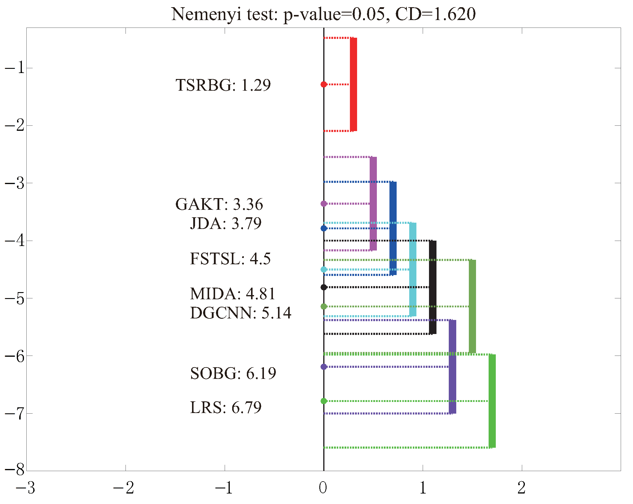
According to the recognition results of different models in Table 1, Table 2 and Table 3, we calculate that the average rankings of them are [3.79, 3.36, 4.81, 4.5, 6.19, 5.14, 6.79, 1.29]. Based on (37) and (38), we obtain the value of variable ${\tau }_{\mathcal{F}}$ is 35.682. If the significance level $\alpha$ is 0.05, then the critical value of Friedman test is 2.0416, which can be obtained through MATLAB expression ‘$icdf$(‘F’, $\alpha ,K-1,(K-1)\ast (N-1))$’ [49]. Since 35.682 is far greater than 2.0416, the assumption “the performance of all models is the same” is rejected. It is necessary to further distinguish the algorithms through the Nemenyi test-based post-hoc test. The results are shown in Figure 2. The models are sorted based on the value of average ranking $r_i$ and the model with higher ranking is closer to the figure top. The length of the corresponding vertical line of these models is called the critical distance (CD), whose value 1.620 is calculated by

$$CD=q_{\alpha }\sqrt{{\displaystyle \frac{K(K+1)}{6N}}},$$

(39)

where the critical value $q_{\alpha }$ is 3.031 when $\alpha =0.05$. We can judge whether there are significant differences between models by whether there are overlaps in the vertical lines corresponding to the models in Figure 2. For example, the rank value of TSRBG is 1.29 while it is 3.36 for GAKT, the gap between them is 2.07, which is greater than the CD value 1.620, so there is no overlap between their corresponding vertical lines. Therefore, the TSRBG is significantly better than GAKT in the cross-subject EEG emotion recognition tasks. Similar analysis can be performed on the other models.

Further, the average recognition results of these models are reorganized by confusion matrices to analyze the recognition performance of each model in each emotional state. The results are shown in Figure 3. We find that TSRBG has a high average recognition accuracy of 82.48% in neutrality state, which is the highest recognition accuracy among the four kinds of emotional states. The proportions of the neutral EEG samples were wrongly divided into sadness, fear, and happiness by 6.90%, 6.56%, and 4.06%, respectively. Compared with the other models, the recognition accuracies of the sadness and neutrality states were significantly improved by TSRBG. For example, the recognition rate of sad EEG emotional states was improved by at least 16.85% compared with the other models. Moreover, the recognition accuracy of the fear emotion category was improved slightly, at 3.45%.

3.4. Subspace Analysis and Mining

In this work, the process of EEG feature transfer is to seek dual subspaces, which are expected to reduce distribution differences between the source and the target domain data as much as possible. For each domain, subspace data representation is obtained by projecting the original data with a projection matrix. In order to intuitively reflect the alignment effect of two domain data in the subspace, we use the t-SNE method [50] to visualize two groups of experimental data before and after alignment. As shown in Figure 4, we see that the data distributions of source and target domain in the subspace have been effectively aligned.

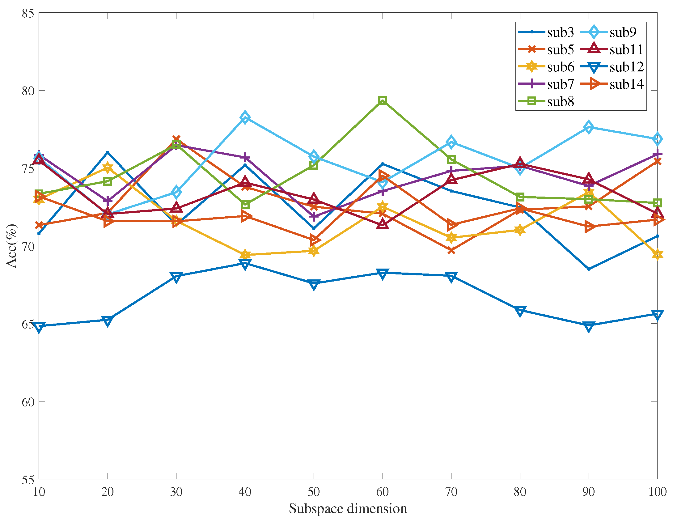
The subspace feature dimension is p. In order to obtain the subspace dimension suitable for data distribution alignment, we show the change of model recognition accuracy with the adjustment of subspace dimension in Figure 5. It is observed that TSRBG is generally insensitive to the subspace dimension. When the subspace dimension is adjusted within the interval [30, 60], TSRBG generally have satisfactory recognition accuracies.

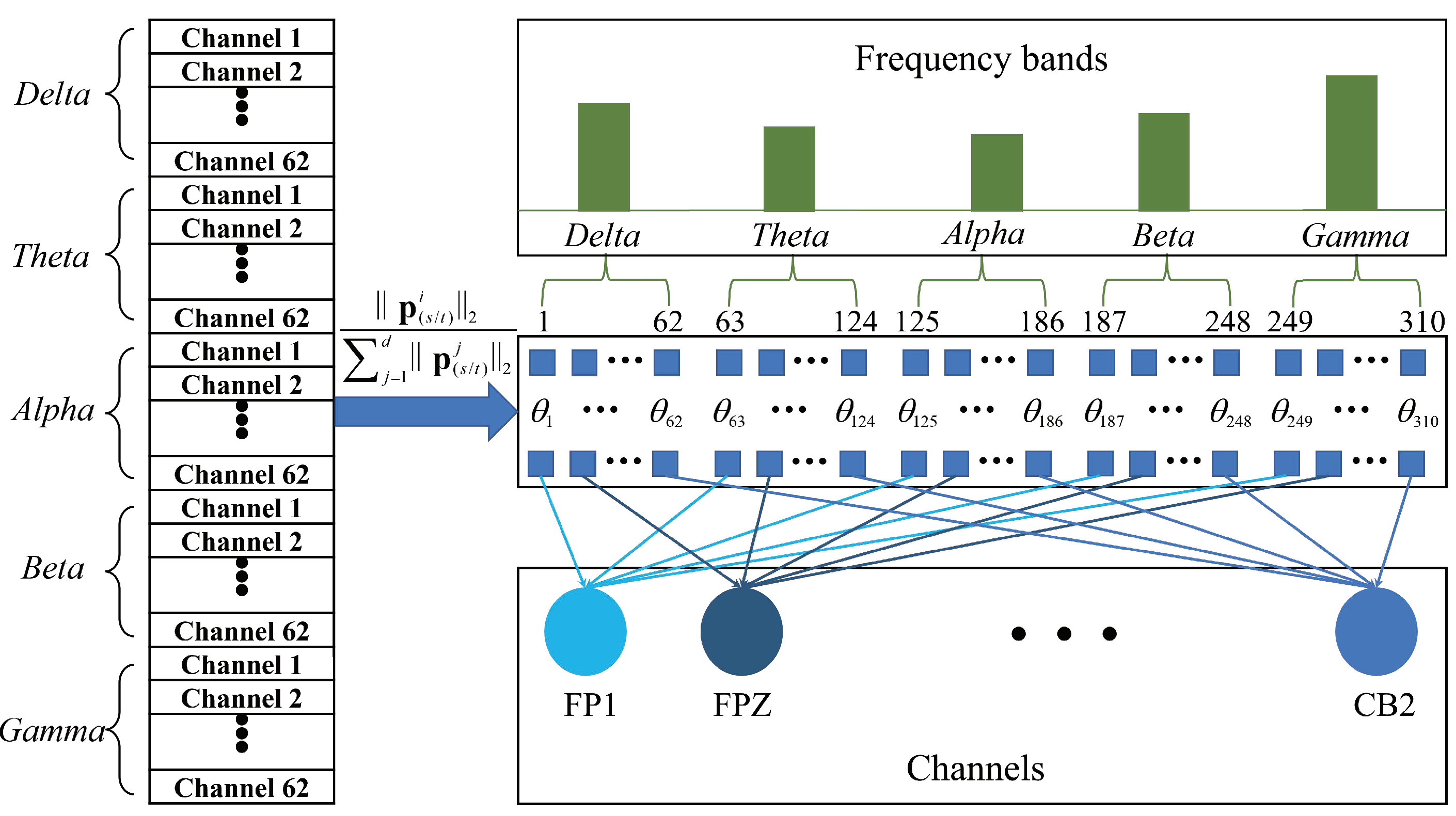
From the perspective of transfer learning, the subspace should reserve the common information and exclude the non-common information between subjects; that is, in the learned subspace, the common components between the source and the target domain should be preserved while the subject-dependent components should be excluded. The subject-independent common components are considered as the intrinsic component of emotion that does not change between subjects. The subject-dependent non-common components are considered as the unique external information of different subjects. From the perspective of EEG features, the subject-independent common EEG features should have larger weights and contribute more to cross-subject emotion recognition. By contrast, the subject-dependent non-common EEG features should have smaller weights and contribute less in cross-subject emotion recognition. If we can quantify the importance of different EEG feature dimensions, according to the corresponding relationship between EEG feature dimension and frequency band [51], the common EEG activation patterns in cross-subject emotion recognition can be explored.

We assume that ${{\theta }_s}_i$ and ${{\theta }_t}_i$ are the importance measurement factors of the i-dimensional features of the source and target domain respectively. Based on the ${\ell }_{2,1}$-norm feature selection theory [52], ${{\theta }_s}_i$ and ${{\theta }_t}_i$ can be obtained by calculating the normalized ${\ell }_2$-norm of the i-row vector of the subspace projection matrix of the source and target domain, respectively. That is,

$${{\theta }_{(s/t)}}_i={\displaystyle \frac{\parallel {{\mathbf{p}}_{(s/t)}}^i{\parallel }_2}{{\sum }_{j=1}^d{\parallel {{\mathbf{p}}_{(s/t)}}^j\parallel }_2}},$$

(40)

where ${{\mathbf{p}}_{(s/t)}}^i$ is the i-th row vector of the subspace projection matrix. Then, we can quantitatively calculate the importance of the a-th frequency band and the l-th channel through

$$\begin{array}{cc}\hfill \omega \left(a\right)& ={\theta }_{(a-1)\ast 62+1}+{\theta }_{(a-1)\ast 62+2}+\cdots +{\theta }_{a\ast 62},\hfill \\ \hfill \psi \left(l\right)& ={\theta }_l+{\theta }_{l+62}+{\theta }_{l+124}+{\theta }_{l+186}+{\theta }_{l+248},\hfill \end{array}$$

(41)

where a = 1, 2, 3, 4, 5 denote the Delta, Theta, Alpha, Beta, and Gamma frequency bands, respectively. l = 1, ⋯, 62 denote the 62 channels, which are FP1, FPZ, ⋯, CB2.

In SEED-IV, the DE features are extracted from five frequency bands and 62 channels. Therefore, the corresponding relationship between the feature importance measurement and different frequency bands (channels) can be established, as shown in Figure 6.

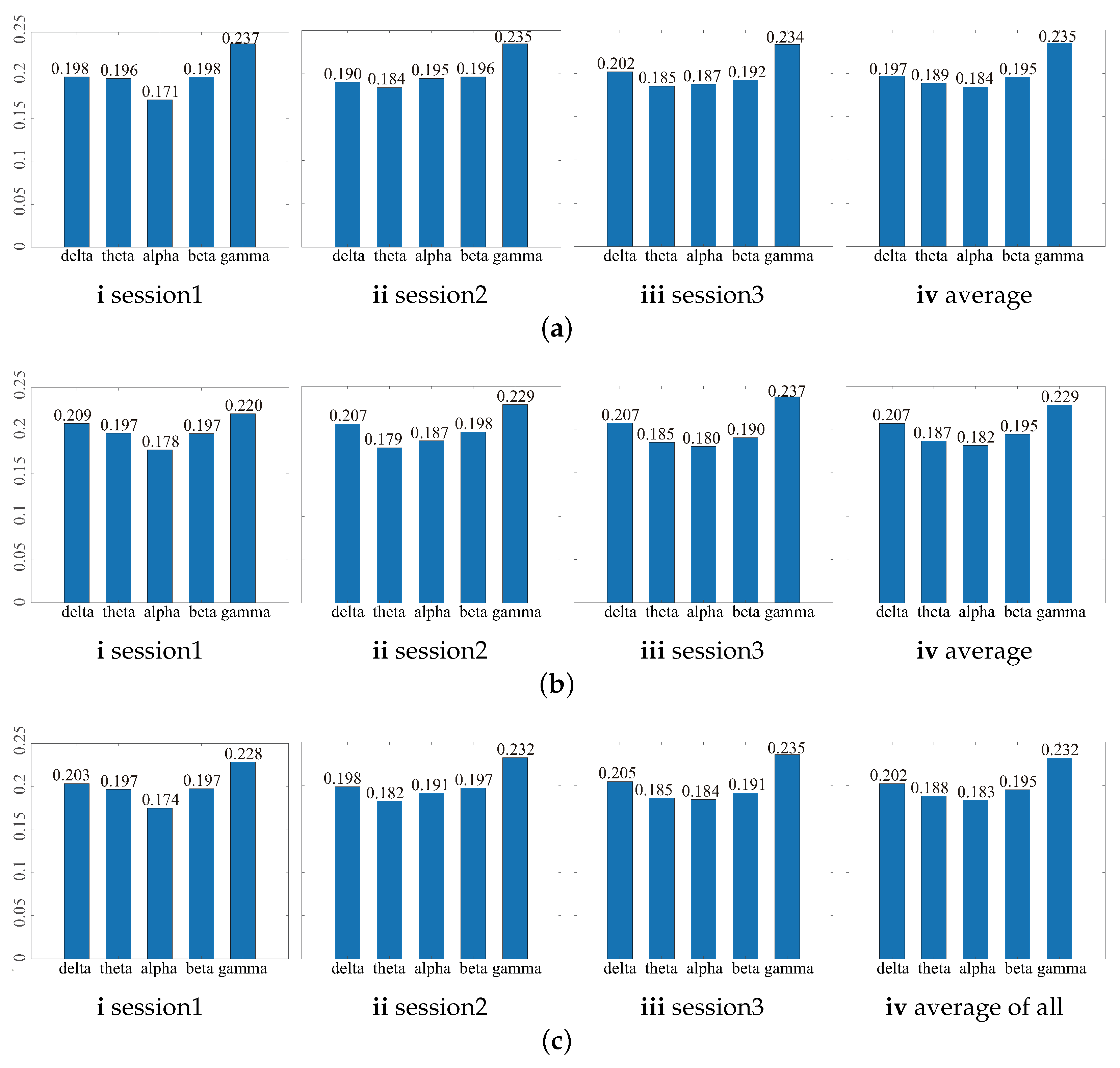
As shown in Figure 7, we quantify the importance of different EEG frequency bands in cross-subject emotion recognition, according to the above analysis. Figure 7a presents the results obtained by analyzing the source projection matrix ${\mathbf{P}}_s$ in three sessions, respectively, and their average results. Figure 7b displays the results obtained by analyzing the target projection matrix ${\mathbf{P}}_t$ in three sessions, and their average result. Figure 7c presents the average results of the source and target domains in three sessions, and the average results of both across all sessions. From the perspective of data-driven and pattern recognition, it is believe that the Gamma frequency band is the most important one in the cross-subject EEG emotion recognition.

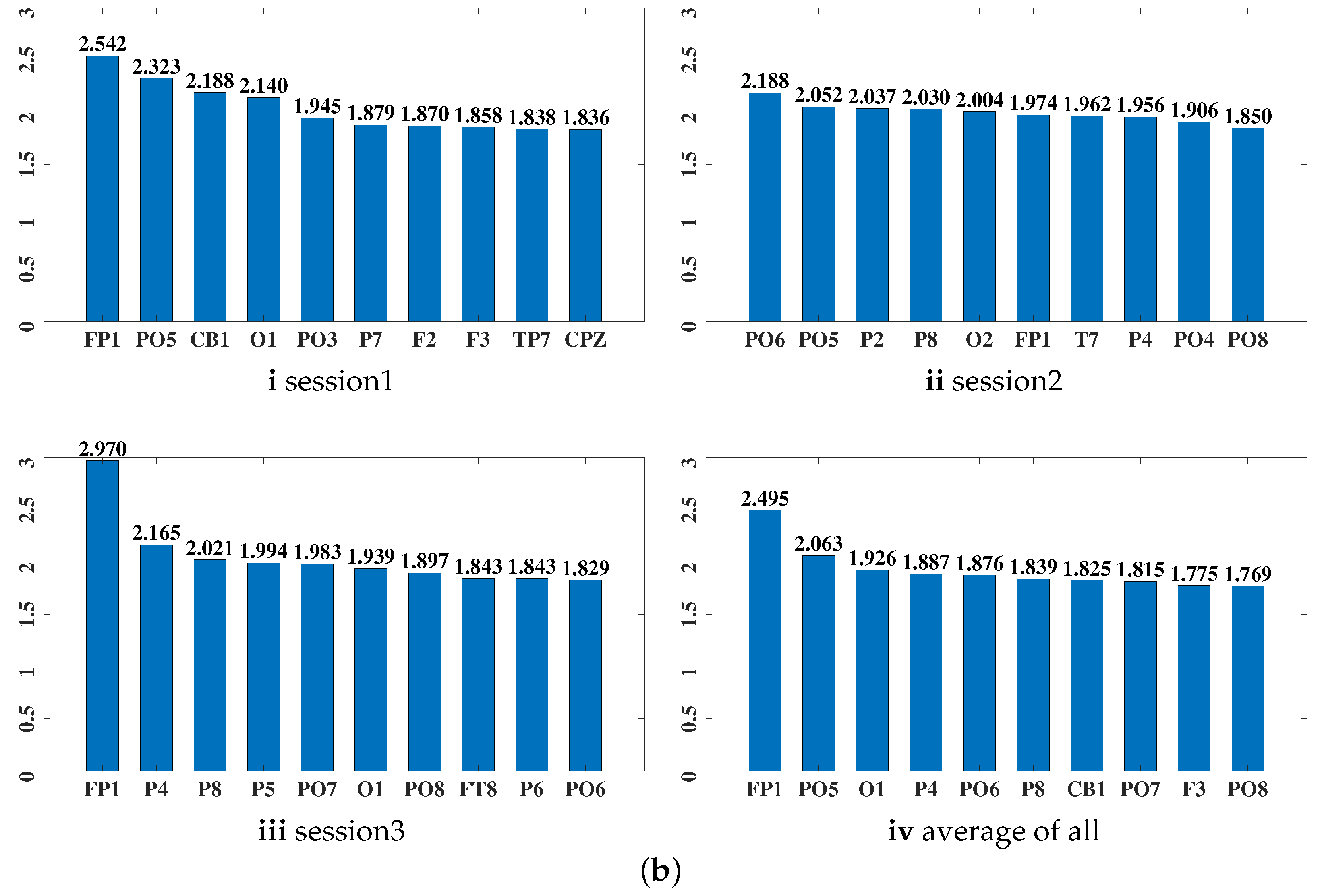
Furthermore, we calculated the importance of different EEG channels, as shown in Figure 8. In Figure 8a, we showed the importance of each brain region in the form of the brain topographic map. We observed that the position of the left side of the prefrontal lobe had high weight in all results, and believe that this brain region should have higher importance in cross-subject EEG emotion recognition. The top 10 important channels of each session and the overall average are quantitatively analyzed in Figure 8b. We believe that FP1, P06, P05, O1, P4, and P8 are more important for the cross-subject EEG emotion recognition. Considering that the model has good performance for sadness and neutral EEG emotional states, the above brain region and channels might be more closely related to these two emotional states.

4. Conclusions

In this paper, we proposed a new model termed TSRBG for cross-subject emotion recognition from EEG, whose main merits are generally summarized as follows. (1) The unification of the feature domain adaptation and the target domain label estimation was effectively realized in a unified framework. Better-aligned source and target data can effectively improve the target domain label estimation performance; in turn, more accurately estimated target domain label information can better facilitate the modeling of conditional distribution modeling, leading to better domain adaptation performance. (2) The intra- and inter-domain connections were investigated based on the subspace aligned data, which formulated a bi-model fusion strategy for target domain label estimation, leading to significantly better recognition accuracy. (3) The learned subspace of TSRBG provided us with a quantitative way to explore the key EEG frequency bands and channels in emotional expression. The experimental results on the SEED-IV data set demonstrated that: (1) The joint learning mode in TSRBG effectively improved the cross-subject EEG emotion state recognition performance; (2) The Gamma frequency band and the prefrontal brain region are identified as more important components in emotion expression.

References

1. Beldoch, M. Sensitivity to expression of emotional meaning in three modes of communication. In The Communication of Emotional Meaning; McGraw-Hill: New York, NY, USA, 1964; pp. 31–42. [Google Scholar]
2. Salovey, P.; Mayer, J.D. Emotional intelligence. Imagin. Cogn. Personal. 1990, 9, 185–211. [Google Scholar] [CrossRef]
3. Chen, L.; Wu, M.; Pedrycz, W.; Hirota, K. Emotion Recognition and Understanding for Emotional Human-Robot Interaction Systems; Springer: Cham, Switzerland, 2020; pp. 1–247. [Google Scholar]
4. Papero, D.; Frost, R.; Havstad, L.; Noone, R. Natural systems thinking and the human family. Systems 2018, 6, 19. [Google Scholar] [CrossRef] [Green Version]
5. Li, W.; Huan, W.; Hou, B.; Tian, Y.; Zhang, Z.; Song, A. Can emotion be transferred?—A review on transfer learning for EEG-Based Emotion Recognition. IEEE Trans. Cogn. Dev. Syst. 2021. [Google Scholar] [CrossRef]
6. Nie, Z.; Wang, X.; Duan, R.; Lu, B. A survey of emotion recognition based on EEG. Chin. J. Biomed. Eng. 2012, 31, 12. [Google Scholar]
7. Ko, B.C. A brief review of facial emotion recognition based on visual information. Sensors 2018, 18, 401. [Google Scholar] [CrossRef] [PubMed]
8. Akçay, M.B.; Oğuz, K. Speech emotion recognition: Emotional models, databases, features, preprocessing methods, supporting modalities, and classifiers. Speech Commun. 2020, 116, 56–76. [Google Scholar] [CrossRef]
9. Alswaidan, N.; Menai, M.E.B. A survey of state-of-the-art approaches for emotion recognition in text. Knowl. Inf. Syst. 2020, 62, 2937–2987. [Google Scholar] [CrossRef]
10. Khare, S.K.; Bajaj, V.; Sinha, G.R. Adaptive tunable Q wavelet transform-based emotion identification. IEEE Trans. Instrum. Meas. 2020, 69, 9609–9617. [Google Scholar] [CrossRef]
11. Becker, H.; Fleureau, J.; Guillotel, P.; Wendling, F.; Merlet, I.; Albera, L. Emotion recognition based on high-resolution EEG recordings and reconstructed brain sources. IEEE Trans. Affect. Comput. 2020, 11, 244–257. [Google Scholar] [CrossRef]
12. Wang, H.; Pei, Z.; Xu, L.; Xu, T.; Bezerianos, A.; Sun, Y.; Li, J. Performance enhancement of P300 detection by multiscale-CNN. IEEE Trans. Instrum. Meas. 2021, 70, 1–12. [Google Scholar] [CrossRef]
13. Hondrou, C.; Caridakis, G. Affective, natural interaction using EEG: Sensors, application and future directions. In Lecture Notes in Computer Science, Proceedings of the Artificial Intelligence: Theories and Applications—7th Hellenic Conference on AI (SETN 2012), Lamia, Greece, 28–31 May 2012; Maglogiannis, I., Plagianakos, V.P., Vlahavas, I.P., Eds.; Springer: Berlin/Heidelberg, Germany, 2012; Volume 7297, pp. 331–338. [Google Scholar] [CrossRef] [Green Version]
14. Marei, A.; Yoon, S.A.; Yoo, J.U.; Richman, T.; Noushad, N.; Miller, K.; Shim, J. Designing feedback systems: Examining a feedback approach to facilitation in an online asynchronous professional development course for high school science teachers. Systems 2021, 9, 10. [Google Scholar] [CrossRef]
15. Mammone, N.; De Salvo, S.; Bonanno, L.; Ieracitano, C.; Marino, S.; Marra, A.; Bramanti, A.; Morabito, F.C. Brain network analysis of compressive sensed high-density EEG signals in AD and MCI subjects. IEEE Trans. Ind. Inform. 2018, 15, 527–536. [Google Scholar] [CrossRef]
16. Murugappan, M.; Rizon, M.; Nagarajan, R.; Yaacob, S.; Hazry, D.; Zunaidi, I. Time-frequency analysis of EEG signals for human emotion detection. In Proceedings of the 4th Kuala Lumpur International Conference on Biomedical Engineering 2008, Kuala Lumpur, Malaysia, 25–28 June 2008; Springer: Berlin/Heidelberg, Germany, 2008; pp. 262–265. [Google Scholar]
17. Thejaswini, S.; Ravi Kumar, K.M.; Aditya Nataraj, J.L. Analysis of EEG based emotion detection of DEAP and SEED-IV databases using SVM. SSRN Electron. J. 2019, 8, 576–581. [Google Scholar]
18. Li, X.; Song, D.; Zhang, P.; Zhang, Y.; Hou, Y.; Hu, B. Exploring EEG features in cross-subject emotion recognition. Front. Neurosci. 2018, 12, 162. [Google Scholar] [CrossRef] [PubMed] [Green Version]
19. Ali Olamat, P.O.; Atasever, S. Deep learning methods for multi-channel EEG-based emotion recognition. Int. J. Neural Syst. 2022, 32, 2250021. [Google Scholar] [CrossRef]
20. Lew, W.C.L.; Wang, D.; Shylouskaya, K.; Zhang, Z.; Lim, J.H.; Ang, K.K.; Tan, A.H. EEG-based emotion recognition using spatial-temporal representation via Bi-GRU. In Proceedings of the 2020 42nd Annual International Conference of the IEEE Engineering in Medicine & Biology Society (EMBC), Montreal, QC, Canada, 20–24 July 2020; pp. 116–119. [Google Scholar]
21. Gong, S.; Xing, K.; Cichocki, A.; Li, J. Deep learning in EEG: Advance of the last ten-year critical period. IEEE Trans. Cogn. Dev. Syst. 2022, 14, 348–365. [Google Scholar] [CrossRef]
22. Li, J.; Qiu, S.; Du, C.; Wang, Y.; He, H. Domain adaptation for EEG emotion recognition based on latent representation similarity. IEEE Trans. Cogn. Dev. Syst. 2020, 12, 344–353. [Google Scholar] [CrossRef]
23. Gong, B.; Shi, Y.; Sha, F.; Grauman, K. Geodesic flow kernel for unsupervised domain adaptation. In Proceedings of the IEEE Conference on Computer Vision and Pattern Recognition, Providence, RI, USA, 16–21 June 2012; pp. 2066–2073. [Google Scholar]
24. Yan, K.; Kou, L.; Zhang, D. Learning domain-invariant subspace using domain features and independence maximization. IEEE Trans. Cybern. 2018, 48, 288–299. [Google Scholar] [CrossRef] [Green Version]
25. Li, Y.; Fu, B.; Li, F.; Shi, G.; Zheng, W. A novel transferability attention neural network model for EEG emotion recognition. Neurocomputing 2021, 447, 92–101. [Google Scholar] [CrossRef]
26. Zheng, W.L.; Lu, B.L. Investigating critical frequency bands and channels for EEG-based emotion recognition with deep neural networks. IEEE Trans. Auton. Ment. Dev. 2015, 7, 162–175. [Google Scholar] [CrossRef]
27. Zheng, W.L.; Zhu, J.Y.; Lu, B.L. Identifying stable patterns over time for emotion recognition from EEG. IEEE Trans. Affect. Comput. 2017, 10, 417–429. [Google Scholar] [CrossRef] [Green Version]
28. Quan, X.; Zeng, Z.; Jiang, J.; Zhang, Y.; Lu, B.; Wu, D. Physiological signals based affective computing: A systematic review. Acta Autom. Sin. 2021, 47, 1769–1784. (In Chinese) [Google Scholar]
29. Suhaimi, N.S.; Mountstephens, J.; Teo, J. EEG-based emotion recognition: A state-of-the-art review of current trends and opportunities. Comput. Intell. Neurosci. 2020, 2020, 1–19. [Google Scholar] [CrossRef] [PubMed]
30. Lu, B.; Zhang, Y.; Zheng, W. A survey of affective brain-computer interface. Chin. J. Intell. Sci. Technol. 2021, 3, 36–48. (In Chinese) [Google Scholar]
31. Niu, S.; Liu, Y.; Wang, J.; Song, H. A decade survey of transfer learning (2010–2020). IEEE Trans. Artif. Intell. 2020, 1, 151–166. [Google Scholar] [CrossRef]
32. Zhuang, F.; Qi, Z.; Duan, K.; Xi, D.; Zhu, Y.; Zhu, H.; Xiong, H.; He, Q. A comprehensive survey on transfer learning. Proc. IEEE 2020, 109, 43–76. [Google Scholar] [CrossRef]
33. Zheng, W.L.; Lu, B.L. Personalizing EEG-based affective models with transfer learning. In Proceedings of the 25th International Joint Conference on Artificial Intelligence, New York, NY, USA, 9–15 July 2016; pp. 2732–2738. [Google Scholar]
34. Zhou, R.; Zhang, Z.; Yang, X.; Fu, H.; Zhang, L.; Li, L.; Huang, G.; Dong, Y.; Li, F.; Liang, Z. A novel transfer learning framework with prototypical representation based pairwise learning for cross-subject cross-session EEG-based emotion recognition. arXiv 2022, arXiv:2202.06509. [Google Scholar]
35. Bahador, N.; Kortelainen, J. Deep learning-based classification of multichannel bio-signals using directedness transfer learning. Biomed. Signal Process. Control 2022, 72, 103300. [Google Scholar] [CrossRef]
36. Jayaram, V.; Alamgir, M.; Altun, Y.; Scholkopf, B.; Grosse-Wentrup, M. Transfer learning in brain-computer interfaces. IEEE Comput. Intell. Mag. 2016, 11, 20–31. [Google Scholar] [CrossRef] [Green Version]
37. Ding, Z.; Li, S.; Shao, M.; Fu, Y. Graph adaptive knowledge transfer for unsupervised domain adaptation. In Proceedings of the European Conference on Computer Vision, Munich, Germany, 8–14 September 2018; pp. 37–52. [Google Scholar]
38. Lan, Z.; Sourina, O.; Wang, L.; Scherer, R.; Müller-Putz, G.R. Domain adaptation techniques for EEG-based emotion recognition: A comparative study on two public datasets. IEEE Trans. Cogn. Dev. Syst. 2019, 11, 85–94. [Google Scholar] [CrossRef]
39. Cui, J.; Jin, X.; Hu, H.; Zhu, L.; Ozawa, K.; Pan, G.; Kong, W. Dynamic Distribution Alignment with Dual-Subspace Mapping For Cross-Subject Driver Mental State Detection. IEEE Trans. Cogn. Dev. Syst. 2021. [Google Scholar] [CrossRef]
40. Gretton, A.; Sriperumbudur, B.; Sejdinovic, D.; Strathmann, H.; Balakrishnan, S.; Pontil, M.; Fukumizu, K. Optimal kernel choice for large-scale two-sample tests. In Curran Associates, Incorporated, Proceedings of the 26th Annual Conference on Neural Information Processing Systems (NIPS 2012); Pereira, F., Burges, C., Bottou, L., Weinberger, K., Eds.; Curran Associates, Incorporated: Lake Tahoe, NV, USA, 2012; Volume 25, pp. 1205–1213. [Google Scholar]
41. Abdi, H.; Williams, L.J. Principal component analysis. Wiley Interdiscip. Rev. Comput. Stat. 2010, 2, 433–459. [Google Scholar] [CrossRef]
42. Bartels, R.H.; Stewart, G.W. Solution of the matrix equation AX + XB = C [F4]. Commun. ACM 1972, 15, 820–826. [Google Scholar] [CrossRef]
43. Peng, Y.; Zhu, X.; Nie, F.; Kong, W.; Ge, Y. Fuzzy graph clustering. Inf. Sci. 2021, 571, 38–49. [Google Scholar] [CrossRef]
44. Zheng, W.L.; Liu, W.; Lu, Y.; Lu, B.L.; Cichocki, A. Emotionmeter: A multimodal framework for recognizing human emotions. IEEE Trans. Cybern. 2018, 49, 1110–1122. [Google Scholar] [CrossRef]
45. Long, M.; Wang, J.; Ding, G.; Sun, J.; Yu, P.S. Transfer feature learning with joint distribution adaptation. In Proceedings of the IEEE International Conference on Computer Vision, Sydney, NSW, Australia, 1–8 December 2013; pp. 2200–2207. [Google Scholar]
46. Song, P.; Zheng, W. Feature selection based transfer subspace learning for speech emotion recognition. IEEE Trans. Affect. Comput. 2018, 11, 373–382. [Google Scholar] [CrossRef]
47. Nie, F.; Wang, X.; Deng, C.; Huang, H. Learning a structured optimal bipartite graph for co-clustering. In Proceedings of the 31st International Conference on Neural Information Processing Systems, Long Beach, CA, USA, 4–9 December 2017; pp. 4132–4141. [Google Scholar]
48. Song, T.; Zheng, W.; Song, P.; Cui, Z. EEG Emotion Recognition Using Dynamical Graph Convolutional Neural Networks. IEEE Trans. Affect. Comput. 2020, 11, 532–541. [Google Scholar] [CrossRef] [Green Version]
49. Zhou, Z. Machine Learning Beijing; Tsinghua University Press: Beijing, China, 2016; pp. 42–44. [Google Scholar]
50. Van der Maaten, L.; Hinton, G. Visualizing data using t-SNE. J. Mach. Learn. Res. 2008, 9, 2579–2605. [Google Scholar]
51. Peng, Y.; Qin, F.; Kong, W.; Ge, Y.; Nie, F.; Cichocki, A. GFIL: A unified framework for the importance analysis of features, frequency bands and channels in EEG-based emotion recognition. IEEE Trans. Cogn. Dev. Syst. 2021. [Google Scholar] [CrossRef]
52. Nie, F.; Huang, H.; Cai, X.; Ding, C. Efficient and robust feature selection via joint 2,1-norms minimization. In Proceedings of the 23rd International Conference on Neural Information Processing Systems, Vancouver, BC, Canada, 6–9 December 2010; Volume 2, pp. 1813–1821. [Google Scholar]
Figure 1. The overall framework of TSRBG.
Systems 10 00111 g001
Figure 2. Nemenyi test on the emotion recognition results of the compared models in our experiments. The critical distance value is 1.620.
Systems 10 00111 g002
Figure 3. The recognition results organized by confusion matrices.
Systems 10 00111 g003
Figure 4. Source and target data distributions. (a) Original space of session2 subject8; (b) subspace of session2 subject8; (c) original space of session3 subject12; (d) subspace of session3 subject12.
Systems 10 00111 g004
Figure 5. Recognition performance of TSRBG in terms of different subspace dimensions.
Systems 10 00111 g005
Figure 6. The framework of emotion activation mode analysis.
Systems 10 00111 g006
Figure 7. Quantitative importance measures of EEG frequency bands in emotion expression. (a) Source domain; (b) Target domain; (c) Average.
Systems 10 00111 g007
Figure 8. Critical brain regions correlated to emotion expression and the top 10 EEG channels. (a) Critical brain regions; (b) Top 10 EEG channels (%).
Systems 10 00111 g008aSystems 10 00111 g008b