1. Introduction
Taxation for meeting public expenditure is an age-old norm that dates to the medieval times when the sovereign took away a part of the crop from the farmers and relied on a feudal system to use serf labor in the name of the ruler. Treasuries and granaries were an integral part of the sovereign infrastructure to horde wealth and food grains collected through revenue officials. Later, precious commodities became a way to exchange goods and services and to pay taxes. It has also been reported in the history of taxation that some sovereigns issued base metal tokens and promissory notes in return for goods and services. These tokens and notes could be used later to pay taxes and they as well began to be traded in the everyday exchange of goods and services, which laid the foundation of the fiat currency system. The origins of money and its evolution into fiat currency are eloquently discussed in literature [
1,
2] and are not further elaborated in this paper which is focused on the relevance of the present-day tax regimens to the fiat currency system and exploring ways to reform them.
Even though fiat currency has now become the norm and the modern money theory [
3], built on its premises is quite widely disseminated [
4,
5,
6], the budgeting operations of the governments continue to use the treasury analogy to run their tax collection and spending functions. They implicitly assume money to be a commodity of value which must first be raised through taxation and stored in the treasury before it can be exchanged for goods and services. The collection of taxes continues to be an expensive and oppressive process that is a legacy of the origins of taxation for supporting autocratic rulers. Its burden remains regressive in spite of advocacy of progressive taxation and the many complex proposals to implement it [
7,
8]. The tax collection process has created rampant corruption in the developing countries where recordkeeping is poor and collection calls for exercise of discretion by the state officials [
9]. It has also created scams that extract ransoms from unknowing victims in the industrialized countries through phishing and fraud [
10]. These taxes are though collected in the form of fiat currency which the sovereign state is empowered to create out of thin air anyways.
It should be recognized that when taxpayers write checks to the treasury, they are reducing the money supply. Since money tokens they are foregoing also reduce their ability to buy goods and services, the tax payments simultaneously reduce the household demand for goods and services. Writing a check to pay for goods and services purchased from a private vendor is different from writing a check to pay taxes. When used for purchases, writing a check reduces the payer’s bank balance, but the money stays in the system since it is transferred to another account. On the other hand, government expenditure funded by fiat money increases money supply in addition to augmenting the demand for goods and services [
11]. Thus, the taxes collected at the outset sponge away excess money in the financial system of the economy, which increases the velocity of money thus slowing down transactions [
12]. Since money also entitles households to buy goods and services, taxes additionally reduce this entitlement, thus limiting economic growth potential [
13]. The statistical evidence for this progression of events, however, varies since a multitude of processes are at work in the economy and causality between two variables can often not be established through association using statistical analysis [
14,
15]. For example, while taxation may exert a downward pressure on prices by limiting household demand, it might simultaneously push prices up by increasing money velocity that also drives up interest rates—increasing capital costs on the supply side.
This paper constructs a parsimonious and aggregate model of the financial system of a sovereign state subsuming both fiscal and monetary interventions. This model is then linked to a one-sector one-factor macroeconomic system adapted from [
16]. The larger model so created is applied to understanding the role of taxation in a fiat currency system. The model is programmed in Stella Architect
1 using system dynamics modeling framework briefly described in
Section 2 and elaborated at length in [
15]. The impact of unlinking public spending from taxation and completely meeting it through deficits is tested using computer simulation. Also, the impact of using taxation and open-market operations for regulating money supply using dynamic feedback control [
17] is investigated. It is demonstrated that taxation must not be seen only as a purely fiscal instrument, but should be tied also to monetary policy [
18]. A market-determined interest rate is proposed as a controller for driving both taxation and open-market operations. Based on the results of computer simulations of the model, a public finance regimen that unlinks taxation from public expenditure and is dynamically controlled by market-determined interest rate is proposed. Limitations of the analysis and further research agendas are outlined.
2. System Dynamics Modeling
System dynamics modeling, originally introduced by Jay Forrester in the1950s to address problems of industrial management [
19], came in limelight with the publication of the
Limits to Growth study [
20] which drew many criticisms [
21,
22]. However, since then, system dynamics has become one of the most popular simulation techniques [
23], and it has been applied to many topics spanning such fields as management [
24], economics [
25,
26], and health [
27].
The underlying computational process in a model representing the microstructure of a theory can be expressed as a set of ordinary nonlinear integral equations, but models are constructed using icons and connections that can be easily assembled using dedicated software such as
ithink,
Stella,
Vensim,
and Powersim 2.
Table 1 shows the icons and the processes they represent in a typical system dynamics model. A rectangle denotes a stock that integrates the flows connected to it. A flow is a rate of change associated with a stock, which may conserve more than one flows. These two types of variables are the basic components of an abstract system implicit in a theory. Information links from stocks to flows define decision rules or policies that drive flows. Intermediate computations transforming information in stocks into policy components are represented by the converter symbol. A converter is an algebraic function of stocks, other converters, and constant parameters. When an intermediate computation involves a nonlinear relationship between two variables, a tilde is added to the converter symbol. The software allows this relationship to be specified graphically.
Once a model has been constructed using these icons, the software allows the modeler to specify initial values of stocks, constant parameters, algebraic functions, and graphical relationships that define each stock, flow, and converter. Non-quantifiable variables can be represented by indices that are tied to tangible variables and normalized with respect to a given ambient condition. The software also allows us to generate the behavior of these models through numerical simulation on a computer. Building confidence in the model involves both structure validation and behavior validation experiments [
28]. Furthermore, simulation experiments are often designed to understand the behavioral patterns arising out of the model structure rather than give point predictions of the future or replicate exact history [
29]. When exploring new regimens with no history, a hypothetical equilibrium may be used to test impact of interventions disturbing that equilibrium as often used in analyzing servomechanisms in engineering systems [
30].
The model of this paper is sketched using the icons of
Table 1 and programmed in
Stella Architect software. The model and its mathematical logic are described in
Section 3. Computer simulations of the model behavior, described in
Section 4, demonstrate implications of the proposed policies. Since the model presented in the paper does not pertain to any specific case and represents an aggregate generic system, an extensive effort to identify parameter spaces unique to classes of model behavior would have little relevance to a more complex real-world, hence it is not attempted. Also, since the policy experiments involve dynamic control driven by
ex post error as in engineering, their outcomes would be relatively insensitive to policy related parameters. Selected sensitivity simulations are nonetheless included to demonstrate this point and discuss the possibilities of improving control by using more complex functions of error.
Section 5 summarizes the results also outlining limitation of this study and suggesting future research directions.
Section 6 concludes the discussion of the paper.
3. A Parsimonious System Dynamics Model of the Public Finance System
The model of this paper portrays an aggregate, homogenous and closed economy.
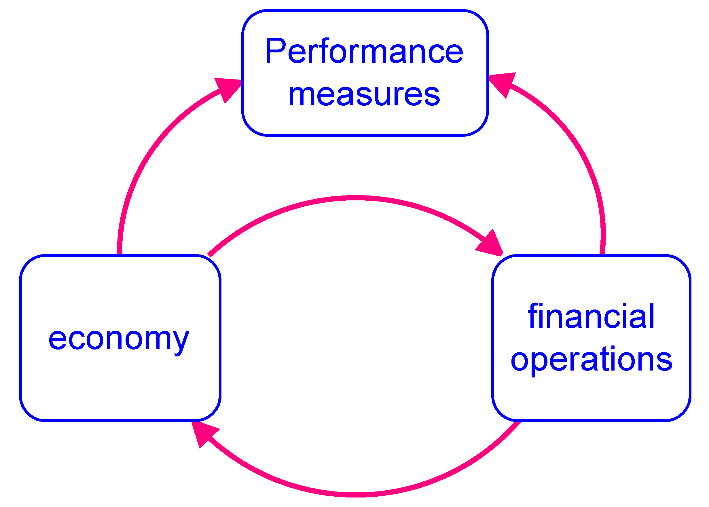
Figure 1 gives a summary view of the model, which includes the macroeconomic processes as well as the financial policy interventions typically exercised by the state institutions.
The module on the left represents an aggregate macroeconomic system while the one on the right is a sub-model of the financial operations manifest in fiscal and monetary interventions. The model behavior over time is described in terms of several representative variables designated as performance measures placed in a separate module to avoid clutter in the model organization. The logic of the three components of the model shown in
Figure 1 is described below.
3.1. Financial Operations
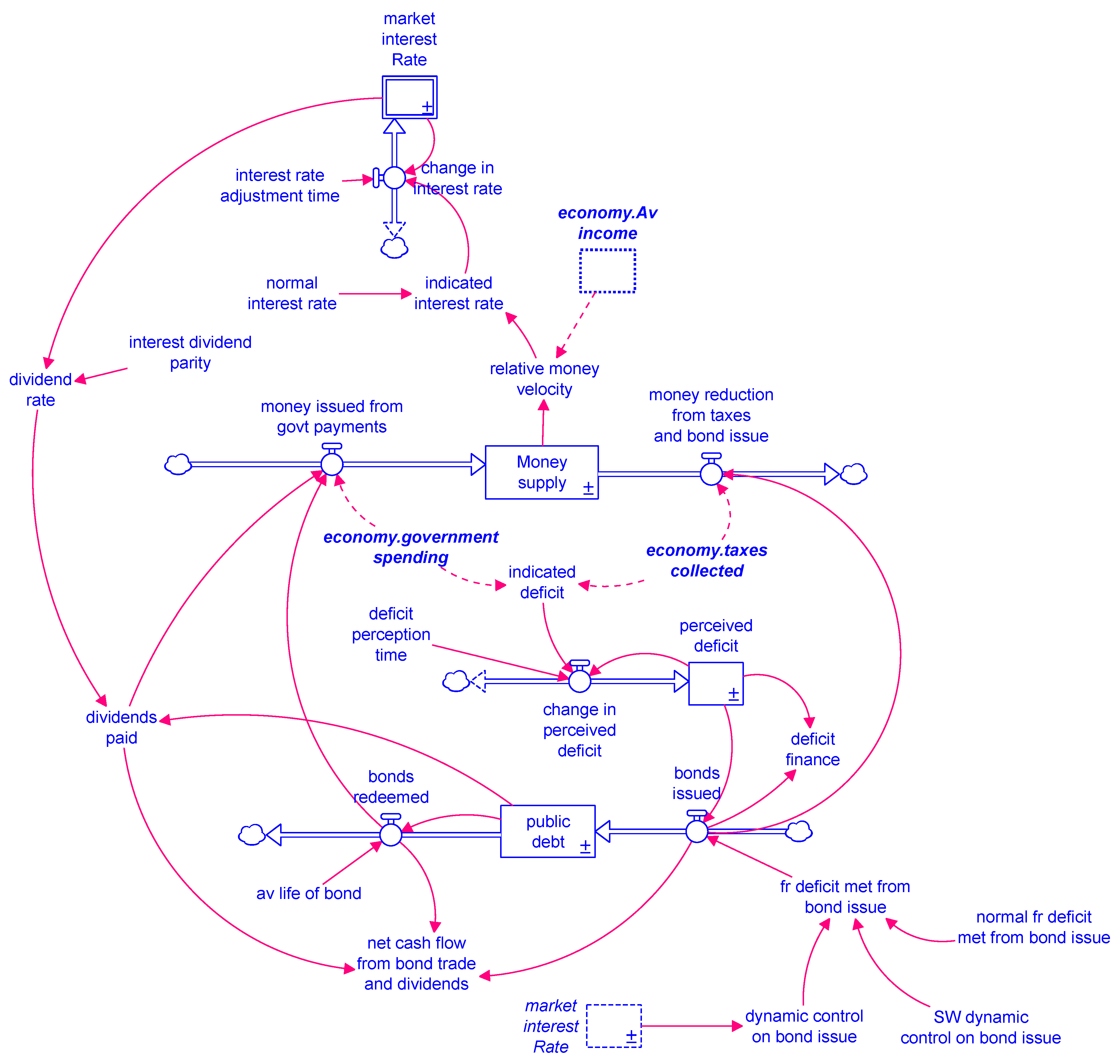
Figure 2 shows the stock and flow structure of the financial operations module. It captures the determination of interest rate based on income velocity of money by a competitive financial market. It also subsumes the government budgetary actions such as taxation and spending, and open market operations such as bond issue and redemption, and how they all affect money supply.
The financial system is represented by three stocks: market interest rate, money supply and public debt. Additionally, indicated deficit consisting of the difference between budgeted government spending and taxation is averaged into a fourth stock of “perceived deficit” to create actionable information.
The central bank actions affect the money supply through buying and selling of government bonds and securities and payment of dividends on public debt. The treasury collects taxes and processes payments of budgeted public spending, which also impact money supply. The bonds issued by the government are viewed as public debt, but they also serve as a secure investment portfolio for the public where it can park surplus cash for future use as well as get guaranteed returns on it. These stocks and the regulatory operations controlling them are described below as integral equations.
3.1.1. Interest Rate
The interest rate adjusts towards an indicated value determined by the relative money velocity that represents the imbalance between money demand created by average income and money supply held in bank accounts and currency notes in circulation.
In the equation above and in the following equations, INIT(·) means the initial value of a variable. It should be recognized that interest rate, as with any other price, can be efficiently linked to money velocity only when it is not fixed by a central bank, but arrived at by a competitive financial market, which is an implicit assumption of Equation (1).
3.1.2. Money Supply
The money supply is an aggregate of currency notes in circulation and the balances held in bank accounts. It is equivalent of money with zero maturity (MZM) that represents the total liquidity of the economy [
31]. Money supply increases through bond and T-bill redemption, payment of dividends on bonds and money creation for meeting government expenditure such as payroll, infrastructure construction, and the purchase of goods and services. Money supply decreases through bond issue and taxation.
The model does not track the change in money supply from changes in saving behavior driven by interest rate that would move money into time deposits, as it would be offset by corresponding changes in lending by the banks. The government can reduce money supply by shredding or erasing money, but it must first capture it from the economy. Taxation is a possible way to capture excess money, although it will also reduce economic growth since it affects household entitlements. In extreme circumstances, governments have removed money by demonetizing certain currency denominations so their holders can no longer exchange them for goods and services, or devaluing money so its holders can exchange the bills they hold with fewer goods and services. Those measures are excluded from the model of this paper.
3.1.3. Perceived Deficit
Although expenditure and taxation are considered fiscal policies, they concomitantly impact money supply, thus affecting the transactions in the economy as monetary policies would. When the government says it has a balanced budget, it really means the money removed from the system through taxes equals the money injected through spending. When the government says it has deficit, it means that the money spent is more than the money removed through tax collection. The difference between taxation and spending is the indicated deficit and its average represents its perceived value that can be acted upon to determine bond issue and deficit finance. Deficit finance implies creating new money for government spending, but whose injection into the economy would also accommodate the transactions demand of a growing economy.
3.1.4. Public Debt
Government bonds held by the public are represented as the stock of public debt. It consists of the currency tokens soaked up from the households and put away until they are redeemed. Bond issue is therefore deflationary in the short run. The outflow from the Public debt stock represents redemption rate after the life of the bond. Bond issue is often sporadic and motivated by the need for funds to spend by a government. From a control perspective, it is proposed to be linked to the market interest rate which mimics money velocity. Several bond issue policies, including a control regimen, are tested. All aim to use public debt to regulate money supply rather than meet government expenditure.
All bonds issued by the government must be redeemed after the promised period. It is assumed that bonds earn a dividend equal to the market interest rate and have an average life of 10 years before they are redeemed. In general, it would also be possible to model a portfolio of short-and long-term bonds, even though such a portfolio is not part of this model.
3.2. The Macroeconomic System
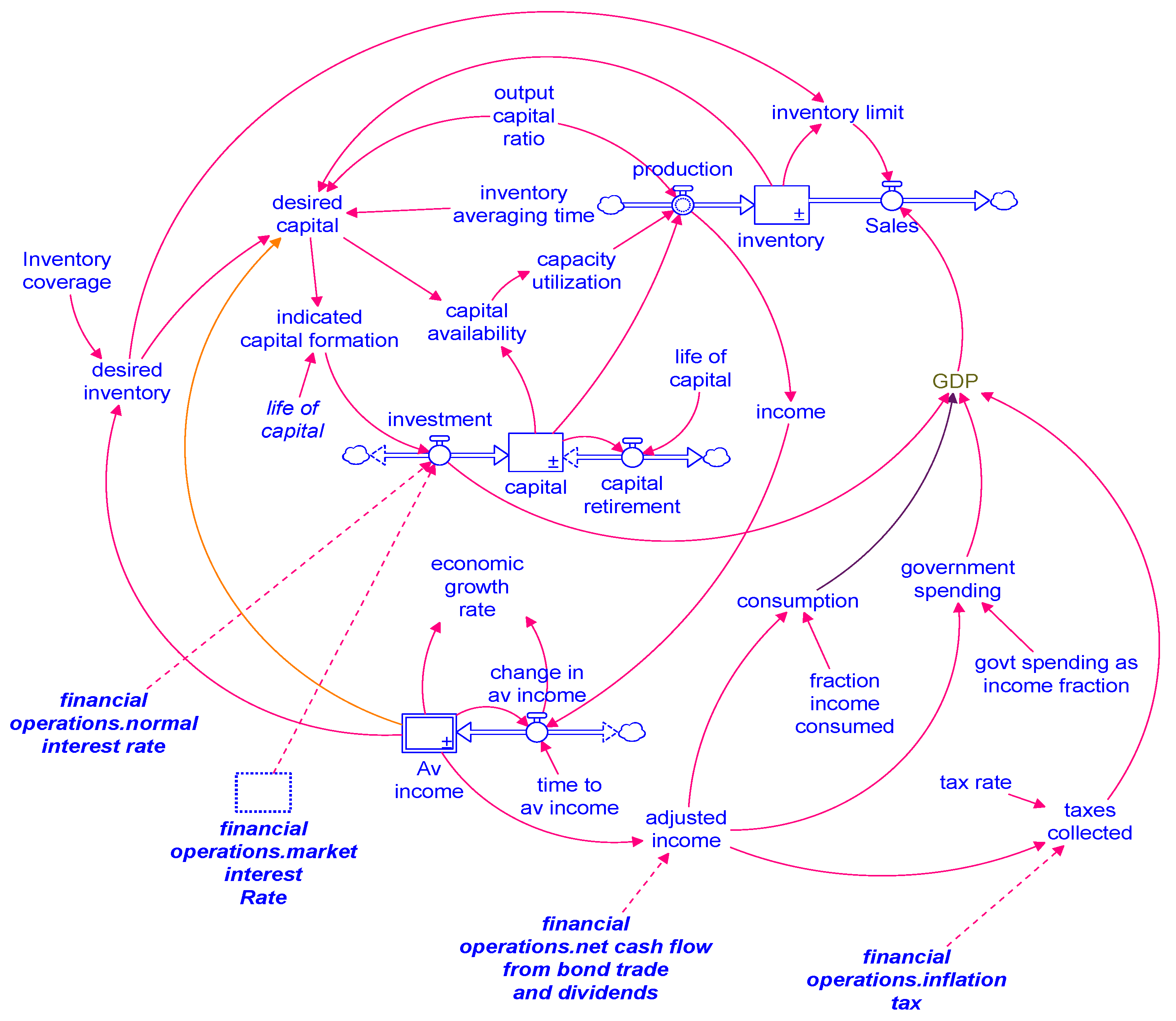
All fiscal and monetary actions affect the economy one way or the other, hence the model of the financial operations is linked with a compact model of the macroeconomic system shown in
Figure 3. It represents a closed and aggregate one-sector and one-factor macroeconomic system subsuming consumption, production, and investment [
32].
3 All flows represent real values measured in dollars/year while capital and inventory are also designated in terms of dollars.
3.2.1. Income
Income is computed on the production side, which depends on capital, capital output ratio, and capacity utilization. On the demand side, it is represented by the quintessential GDP identity consisting of the summation of consumption, investment and government spending less taxes collected. Government spending is assumed to be pegged at a percentage of the national income since a rise in income would entail enlarging the social services infrastructure. The following integral equations describe the stocks and their respective flows in this simple model of the economic system adapted from [
16]:
where income equal production in real terms when the general price level is assumed to remain steady.
3.2.2. Inventory
Inventory separates supply and demand. The general price level (GPL) is not included in the model for simplification, but inventory limitation restricts sales while the unmet demand is not tracked, which implicitly assumes price adjustment to clear any surplus or deficit of demand and sales:
Since money is a legal tender for transactions, a reduction in the household money balance, whether incurred through taxation or by purchase of government bonds) would also reduce demand for goods and services. Thus, both taxation of fiat money and money reduction through bond issue have impacts similar to the medieval taxation practice where tax often constituted a part of the crop or real commodities. Following equations describe the composition of demand and its components:
Taxes collected combine a simplified version of the traditional taxation modeled as a fraction of adjusted income and the suggested version of remedial taxation for inflation control proposed in this paper, which is driven by the market interest rate. For experimentation with the model, either type of taxation can be activated or disabled.
where max inflation tax rate defines an upper bound for such taxation. This limit determines the rate of adjustment of the inflation tax rate in response to the changes in interest rate. Note it can become negative when market interest rate is high. Inflation tax in such a case would be a rebate.
3.2.3. Capital
All production capital is aggregated into a single stock that is increased through investment and decreased through retirement:
In case of an open economy, trade imbalance, together with remittances and factor income flows will create current account balance, which integrates into the national reserves of foreign currency in addition to affecting GDP. Foreign trade, remittances and factor income flows are excluded from the model of this paper, which focusses primarily on the internal financial management of the economy.
3.3. Performance Measures
The model, although not calibrated for any specific case, must be supplied numbers for implementing the numerical simulation process. Its output is also plotted in terms of numbers. The model has many variables and representing all of them in the output would be confusing. Several relative performance measures have therefore been created, which are independent of the size of the economy. These measures are used to compare the various simulations. Not all performance measures are reported in each simulation experiment. These performance measures are discussed below.
3.3.1. Economic Growth Rate
Economic growth rate is computed as a fractional growth rate as follows:
3.3.2. Relative Money Velocity
Relative money velocity is a measure of the adequacy of money supply
It computes to 1.0 in the initial equilibrium when
3.3.3. Market Interest Rate
Market interest rate is the price of money determined by a competitive financial market. It is computed in Equation (1) and initially set at 0.05 corresponding to relative income velocity of 1.0.
3.3.4. Deficit Finance GDP Parity
Deficit finance GDP parity is defined as the ratio of deficit finance to GDP:
It initially computes to zero when there is no deficit.
3.3.5. Public Debt GDP Ratio
Public debt GDP ratio, as the name implies, is the ratio of outstanding public debt to GDP:
This measure keeps track of public debt as a fraction of GDP. If public debt supports welfare expenditure, it indirectly measures private sector contribution to collective good and it can be seen as excess private capital drawn into social projects. This ratio initially computes to zero with no public debt.
3.3.6. Inflation Tax Rate
The proposed inflation tax rate is dynamically controlled by the market interest rate. It is defined in Equation (2) and is initially set at zero, when interest rate is at its initial value of 0.05.
4. Model Behavior
The model is calibrated to initialize in a hypothetical equilibrium, which serves as a point of reference to compare the policy simulations with. It has not been calibrated for any specific case, hence, relative rather than absolute comparison of the performance measures would be meaningful in the simulation experiments that follow. The model is initialized with GDP = 100 units (say billions of dollars), taxes = govt spending set at 10% of average income, no deficit, and no public debt. The model was simulated for 100 years but only 25 years of behavior is shown since thereafter the system soon settles into a new equilibrium.
When taxes are abolished and all government spending is financed by newly minted fiat money, the increased disposable income from not having to pay taxes stimulates the economy into growth. Indeed, deficits extensively fueled postwar recovery in Europe and USA and successfully mitigated economic stagnation [
33]. Since govt spending is tied to income in our model, the economy receives continuous stimulus, and the growth rate rises, tapering off at about 5% (Graph 1 in
Figure 4). In reality, there would be economic cycles of various periodicities arising out of inherent delays in workforce adjustment, over-investment and capital self-ordering [
34]. There would also be constraints arising from resource limitations [
35] and conflict [
36]. The structure for those behaviors is outside of the scope of the model of this paper.
The health of the monetary system is reflected in the simulation representing the relative money velocity (Graph 2), which declines from its designated normal value of 1-tapering off at about 0.5, indicating considerable inflation. Market interest rate (Graph 3), being the true price of money, is strongly correlated with the velocity of money and can serve as an accurate indicator for it since measurement of money velocity is often a challenge. Although the causal relation between the velocity of money and market interest rate is difficult to infer from their association, it makes sense to postulate that price of money would be determined by its availability evident in its velocity, provided interest rates are determined by a competitive lending market and not modified by the central bank
4.
The current deficit as a fraction of GDP (Graph 4) rises at first but then declines slightly over time since growth in national income eventually exceeds the growth in government spending due to multiplier and acceleration effects as postulated by Keynes [
37] and first modeled by Samuelson [
38]. It levels off at a value lower than the fraction of income it is based on, since GDP without taxation will always exceed income.
Subsequent experiments with the model are aimed at creating control processes using open market operations and taxation as remedial instruments that should maintain reasonable economic growth without causing excessive inflation.
4.1. Remedial Open Market Operations for Regulating Money Supply
Open market operations are already quite widely used although for supporting public expenditure [
39]. The first group of experiments aims to assess the impact of open market operations on money supply. Several options subsuming combinations of meeting a part or whole of the deficit by bond issue and applying feedback control using the interest rate deviation from its normal value as a controller are tested. The results of these experiments are summarized in
Figure 5 in which Graphs 1 replicate the results of
Figure 4 and act as the base case for evaluating various policy sets.
The first experiment entails an effort to defray 100% of the perceived deficit through bond issue. Note, bond issue here is not linked to public spending but to deficit. It is therefore meant for soaking away surplus money in the economy and transferring it to public debt. An externality of this process is that surplus private cash, which might otherwise chase speculative portfolios, is drawn and held in a socially beneficial portfolio. The results of this experiment are shown in Graphs 2 in
Figure 5.
When the volume of bond issue completely offsets all deficit, the economic growth rate is considerably reduced since the investment in bonds reduces adjusted income. The concomitant reduction in money supply also increases money velocity, which can further inhibit growth. Bond redemption and dividend payments later stimulate the economy into growth while also decreasing money velocity. Public debt rises as the growing economy calls for increasing deficit finance of public expenditure and eventually tapers off at about 50% of the GDP.
When labeled as public debt, that proportion might appear huge. When seen as a revolving fund that soaks excess money from the market and parks excess entitlements of the wealthy, it seems to mobilize private surplus into supporting public expenditure. It is supported by the wealthy not out of charitable intentions, but due to the profit motive when the dividends are seen to be a low-risk investment. Bond issue therefore can be deemed to play as a voluntary tax that is rewarded by dividends. Such a tax will also be quite progressive as the rich will have more spare cash to invest into the bonds than the poor. Note also, the net cash flow from bond issue, redemption, and bond dividends factors into the calculation of adjusted income as it affects the entitlement of the households. When excess money is soaked away by bond issue, money velocity is at first sustained, but then declines as bond redemption and dividends start adding to the money supply.
When bond issue is set to defray only a part of the deficit (set at 50% in the simulation shown in Graphs 3), economic growth rate improves, while money velocity declines more rapidly than in Graphs 2, but ends up at more or less the same place towards the end of the simulation. Public debt is reduced while deficits continue at a reduced level, but some of the increase in money supply this creates is accommodated by the transactions need of a growing economy.
When bond issue is regulated by the market interest rate, the proportion of deficit met through bond issue can be dynamically controlled and not arbitrarily set. Such a regulatory process is embodied in Graphs 4 of
Figure 5. Economic growth rate in Graphs 4 is only slightly lower than Graphs 3, but money velocity is maintained at a higher level and deficit is considerably reduced. Public debt-GDP parity is higher in Graphs 4 than in Graphs 3. However, as pointed out earlier, internal public debt may point to the extent of privately supported social services, which should not raise concerns.
4.2. Remedial Taxation to Regulate Money Supply
The simulations of the last section have addressed the implications of delinking taxation from public expenditure and meeting the later through deficit financing. The deficit can then be soaked up through open market operations. However, while the monetary authority can sponge away extra cash through open market operations, when the bonds it issues are redeemed, cash is injected back into the economy. Also, the dividends the government must pay on the bonds further inject more cash into the economy. Last, but not least, a growing economy might offer better investment opportunities than government bonds and the demand for bonds may fall short of the new bond issue need dictated by the money regulation process. When excess cash cannot be removed effectively through open market operations, some sort of taxation would be needed to capture it from the economy before it is erased to avoid inflation. A remedial taxation recourse for regulating money supply is explored in this section.
Figure 6 shows three simulations for understanding the use of remedial taxation for regulation of money supply. As in case of bond issue regulation, experimented in the last section, market interest rate is again used as a controller for driving the rate of remedial taxation.
The behavior of four performance measures is shown: economic growth rate, deficit finance GDP parity, relative money velocity and tax rate. Graphs 1 represent the base case from
Figure 4. Note that the inflation tax rate shown in Graph 1 of the inflation tax graphs is hypothetical, since it is calculated, but not applied.
Graphs 2 show the case when remedial taxation is aggressively regulated by market interest rate (max inflation tax rate = 0.5). Indeed, it greatly reduces the deficit and increases the money velocity. However, since it reduces entitlement of the households, it also considerably reduces economic growth rate. The case of moderate inflation taxation regimen (max inflation tax rate = 0.25) is shown in Graphs 3, which exhibit improvement in economic growth rate with a concomitant reduction of money velocity, indicating a higher rate of inflation, which is often equated with implicit taxation [
40].
These experiments show that public expenditure can be unlinked from taxation while remedial taxation driven by a measurable indicator of money velocity can be used to control inflation. It should be noted however that while open market operations can also be used to that end, taxation is not voluntary unlike investment in government bonds. Also, since bonds would most likely draw surplus cash from the rich into public spending, their tax burden will be progressive. On the other hand, a remedial income tax would affect all income cross-sections and if tax rate is flat for simplicity, the taxation process will be regressive. A remedial tax can be slapped on wealth instead of income with impact no different from income tax, but its impact on investment is not investigated by the model of this paper.
It should be noted that when money supply has changed to the desired value, the inflation tax should go to zero. Also, when money is in short supply, a negative tax can be levied in the form of rebate checks mailed out to people or government spending can rise to inject additional money into the economy. A remedial tax would however be highly variable and must not be driven by public expenditure which can often not be changed easily.
4.3. Combining Remedial Open Market Operations and Taxation
The simulations of the last two sections show that the open market operations and remedial taxation are complementary ways to control inflation. Both also change private entitlements that will impact demand. The former however integrates into the stock of public debt, which is in fact a revolving fund that soaks excess money supply from the market and parks excess entitlements of the wealthy.
Through combining open market operations with remedial taxation, a government can first create the money it needs for public spending, then reduce the excess currency so created by bond issue and taxation, both of which must be regulated by the market interest rate. The deficit reduction process driving bond issue does yield a higher level of public debt. In this section, we compare the performance of open market operations, remedial taxation, and their combination.
Figure 7 shows the simulation of these options. As in other simulations, Graphs 1 in
Figure 7 replicate the base run of
Figure 4.
Graphs 2 replicate Graphs 4 of
Figure 5 that embody dynamic control on bond issue driven by market interest rate. Graphs 3 replicate Graphs 3 of
Figure 6 that show the behavior when moderate remedial taxation is driven by market interest rate. Finally, Graphs 4 combine bond issue and remedial taxation, both driven by market interest rate and thus both addressing inflation.
Using dynamic control on bond issue only yields high rates of economic growth but little inflation control (Graphs 2), especially when bond redemption and dividends start injecting money back into the economy. It, however, transfers much of the deficit into public debt. Using dynamic control of inflation taxation (Graphs 3) yields a sustained but lower rate of economic growth as it reduces disposable income. It albeit more effectively sponges away surplus money to control inflation even though it maintains a higher level of deficit since no part of it is transferred into public debt. Using both controls (Graphs 4) yields economic growth rates and money velocity similar to Graphs 3, but with the lowest level of deficit and moderate public debt.
The simultaneous regulation of inflation tax and bond issue, both driven by market interest rate, create compensatory feedback processes that can reduce the sensitivity of parametric variations in each. They also draw both the surplus of the rich and an across board tax into reducing the deficit. This combination can be quite robust even when behavioral responses of an authority implementing the regulation vary within reasonable limits, which can often happen when individuals manning the process change.
4.4. Sensitivity of Policy Parameters
While a sensitivity analysis is an important part of model testing and in the policy context, it helps to identify parameters tied to effective policy intervention, in this case, the proposed policies are based on dynamic control that allows for the system to adjust the magnitude of the intervention iteratively. The last policy experiment described in
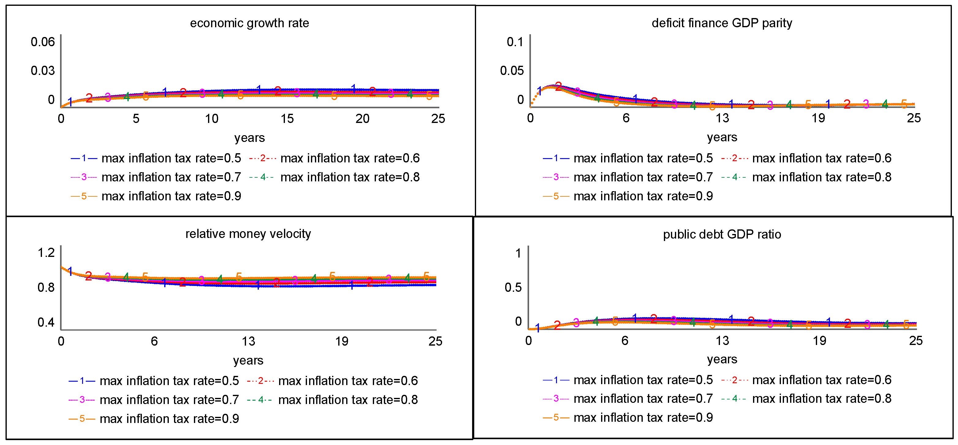
Section 4.3 also explored two compensating negative feedback loops that further reduce sensitivity to parameter values. What really matters for this analysis is recognizing the structure that drives the adjustments. If in the first iteration, a parameter value may lead to a weak adjustment, in the subsequent iteration, the remaining error will force a stronger adjustment. To confirm this assertion, the sensitivity of the outcomes to changes in the inflation tax rate cap (max inflation tax rate in model) in the policy proposed in
Section 4.3 was tested beyond the aggressive level 0.5 simulated in
Figure 6. Note values of 0 and 1 are not included in the sensitivity experiment as 0 would disable the control process in the model while 1 would mean that 100% of disposable income can be taxed, which would never be the case. In fact, all values for the max inflation tax rate beyond 50% are impractical but are included in the sensitivity run to demonstrate the robustness of the control process.
Figure 8 shows the results of this test.
As expected, there is almost no change in the patterns of behavior, while some spread is observed in the steady state values towards the end of the simulation that may arise from the fact that only proportional functions of
ex post error in the market interest rate were used to drive the corrections, which is known to generate steady state error [
41,
42]. Experimentation with more complex functions of error is suggested in
Section 5.2 as a future research direction.
5. Discussion
5.1. All Taxation Can Be Remedial
First proposed by Arthur Pigou, remedial taxation is often used to affect costs and benefits of targeted activities to either encourage or discourage them in modern day economies [
43]. Examples of remedial taxation include carbon taxes to contain environmental degradation, trade tariffs to correct balance of payments, taxes on fossil fuels to shift consumption to alternative energy sources, progressive wealth taxes aimed at reducing income disparities, and taxes on tobacco and alcohol to discourage their use. The operational criteria for implementing environment-related taxes is outlined in [
44]. The dynamic energy basket composition is studied in [
45]. The taxation of unearned income as a tool for remedying income distribution is explored in [
46] and trade tariffs and foreign exchange reserves in the context of the foreign trade regulations are examined in [
47].
The yield from all remedial taxes should decline to a very small amount when the problems they are addressing have been mitigated. Yet, such taxes often become a staple for meeting the budgetary needs of public expenditure. This can be avoided when public spending is met at the outset through money creation while remedial taxes together with open market operations alter money supply by soaking up the excess cash in the system. Government spending when not tied to taxes anymore can remain stable and targeted to increasing public welfare.
The use of dynamic control process applied to the currency instruments presently in use also point towards the possibility of dispensing with all taxation and using programmable electronic currency instruments with taxation built into them. The so-called
blockchain technology for electronic currency is already available, but it must be backed and regulated by a country government if taxation is to be subsumed into it. A discussion on the use of a central bank issued digital currency (CBDC) has already started [
48]. Taxation can be implemented in the currency by building into it a devaluation process driven by the inflation indicators used in our experiments. However, a currency that depreciates over time or through transaction can lose its value as a vehicle of exchange, hence a transaction tax, regulated by market interest rate as discussed in our experiments, would be a better way to sponge away extra currency from the system, which can also be programmed into CBDC. Income tax can be eliminated while the regressivity of the transactions tax can be mitigated by expenditure instruments such as permanent basic income and provision of free healthcare and education. Further research is needed to explore those options.
It is often surmised that a central bank would be able to contain proliferation of money through interest rate changes that are driven by the imbalance between money demand and money supply and drive changes in money supply through precise interventions, which might be a heroic assumption for most countries where central bank actions are often unsystematic, sporadic, and largely ineffective. Interest rate, if it is to represent the true price of money, must be determined by the market. Only then will it precisely follow money velocity. It should be a driver of the monetary policy, not driven by it. Changing it amounts to shooting at the messenger.
5.2. Model Limitations and Future Research Agendas
The economic growth sector of the model presented in this paper at the outset represents a homogenous and closed economy with elastic labor supply. This simple and aggregate model also does not address resource and environmental constraints, allocation inefficiencies manifest in competition between defense and economy, leakages due to corruption and illegal production and the problems arising out of obsolescence of the capital in use. Also, while this simple model helps to understand the role of taxation in a fiat currency system and propose alternative mechanisms for meeting public expenditure. It does not address the implications of maintaining high levels of public debt and cumulative deficit on foreign trade and factor payments. Nor does it incorporate structure for understanding the impact of proposed public finance regimen on labor market dynamics, income distribution, governance, and environment.
It should be recognized that the balance of payments pertaining to foreign trade and factor income transfers is different from public debt, which is a part of the indigenous economic management. A control from the payments balance on trade tariffs can be applied along with the consideration of the value flows accompanying trade. This needs to be further investigated by extending the simple model of the macroeconomic system used in this paper.
The dynamics of income distribution and the challenges they offer for the developing countries are explored in [
49]. The financial policy sector can indeed be linked with a more complex economic system incorporating labor market dynamics, income distribution and trade and factor income flows, which is suggested as a valuable direction for future research. The role of resource and environmental constraints are outlined in [
34], and environmental remediation processes are outlined in [
50]. Allocation inefficiencies and leakages are discussed in [
36]. Elements of these can be included in an extended model of the economy to understand the impact of proposed tax reform.
Finally, the control mechanism used to regulate remedial policy instruments suggested in this paper are simple proportional functions of the controller, which might be the cause of the steady state error in velocity of money and interest rate in the policy simulations. Complex functions of controller used as drivers of correction can possibly alleviate steady state error as well as instability in adjustment [
41,
42]. Further investigation should include experimentation with such functions of error.
Last, but not least, how soon the proposed taxation reform can be adopted in the existing system of institutions is a subject related to the evolution of economic systems and how they are affected by other institutions as outlined in [
51]. Further research may also address the evolution process in the adoption of dynamic control process in taxation systems.
6. Conclusions
Taxation continues to be perceived as necessary for public finance in the tradition of the commodity view of money, while deficit finance has been widely used to support public expenditure even though its use has drawn much debate [
52]. The Gramm-Rudman-Hollings act of 1985 [
53] is a testimony of the continued perception of money as a commodity, which is removed from reality. All politicians have talked about tax reform but have often carried out little more than rearranging chairs on the deck of the Titanic that is sinking in an ocean of confusion about the nature of money we use. Fiat money is already an integral part of the modern-day economies and any tax reform must deal with this fact [
54,
55].
This paper has presented a system dynamic model subsuming the macroeconomic growth processes and the fiscal and monetary policies exercised by the government. It has employed computer simulations to understand the impact of financial management policies and the impact of replacing the expenditure-driven taxation completely with two remedial instruments (i.e., open-market operations and an inflation tax) both regulated through feedback control by a market -determined interest rate. This analysis accepts the universal use of a fiat currency system and explores how the regulatory process can be modified to delink taxation from public expenditure.
A sovereign government can create fiat money tokens to pay for expenditure, while taxation and open market operations sponge excess money away, so monetary inflation is minimized. Taxation and open market operations can therefore be unlinked from public spending and driven not by the need for funds, but by a measure of inflation, which is proposed as the centerpiece of the tax reform in the face of widespread use of fiat money.
When all public spending is met at the outset from deficits that are partly offset by public debt, the public debt indirectly draws the surplus wealth of the rich to fund public expenditure. The wealthy thus support public expenditure though not out of charitable intentions but due to the profit motive when the dividends are seen as a low-risk investment. Taxation might still have a place in the fiat currency system as a remedial process for soaking up surplus money for controlling its velocity. For this, it must be driven by a free-floating interest rate determined by the market, which will reflect the true price of money, rather than by a central bank that may in fact corrupt this indicator by basing it on multiple considerations.
Automating tax collection through depreciation of money can be built into an electronic currency system, but this would discourage its holding and use as a medium of exchange. However, income tax that is most expensive to collect can be dispensed with, while all surplus money is sponged away using a transaction tax and open market operations. Regressivity of transaction tax can be offset by social expenditure policies and transfer payments such as provision of permanent basic income, free education, and universal healthcare.
Remedial taxation driven by a market indicator of discrepancy between goal and existing condition can also be used to address problems such as resource shortages, environmental degradation, income disparities, use of harmful substances, trade imbalances, allocation inefficiencies etc., for which further research on tax reform is proposed.
To close, this article represents a preliminary exploration of taxation as a monetary instrument in the fiat money context and how this mechanism can be implemented using dynamic control to contain inflation. It is expected to stimulate further thinking on this subject rather than being the final word.


