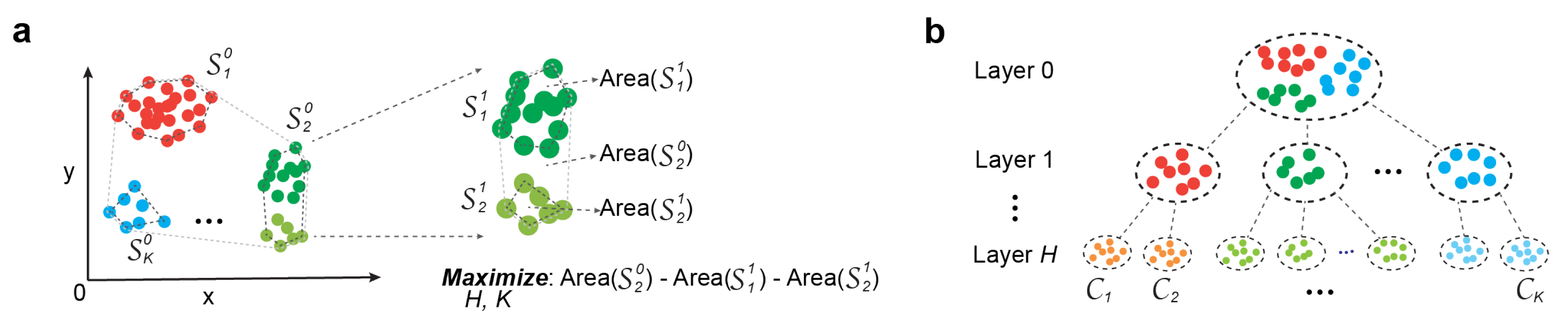
Figure 1.
Illustration of optimization strategies: (a) Convex hull-based optimization. (b) Identification of cell types and their hierarchical organization from scRNA-seq data.
Figure 1.
Illustration of optimization strategies: (a) Convex hull-based optimization. (b) Identification of cell types and their hierarchical organization from scRNA-seq data.
Figure 2.
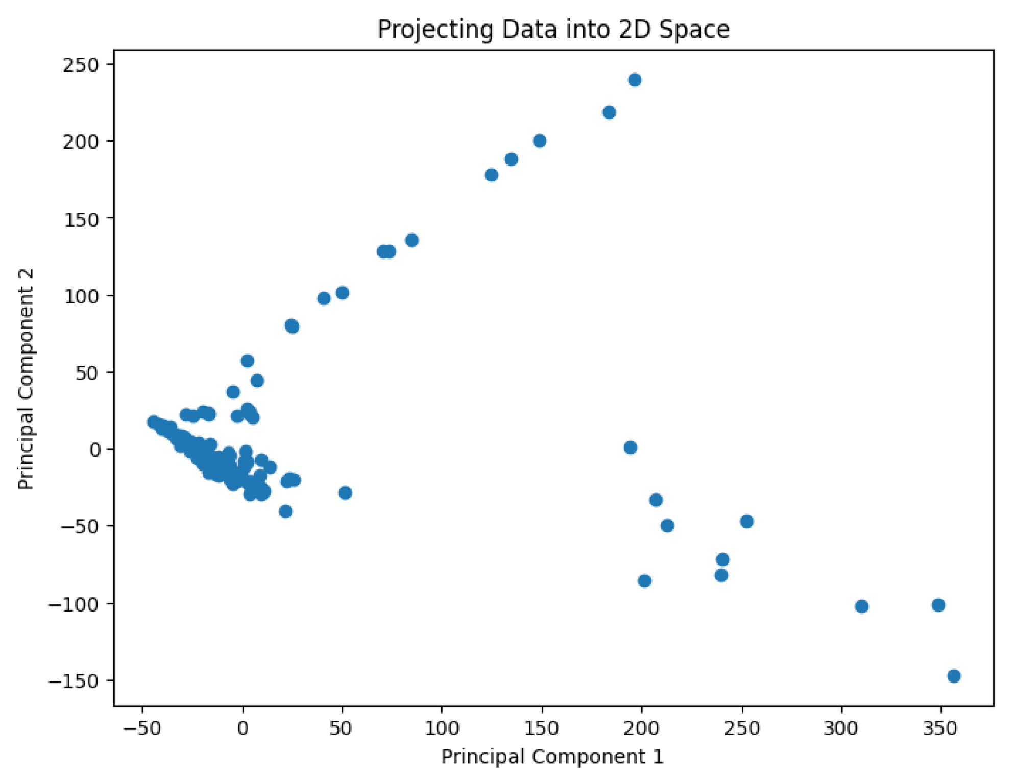
The projected data in the 2D space for the dataset Biase.
Figure 2.
The projected data in the 2D space for the dataset Biase.
Figure 3.
The projected data in the 2D space for the dataset Deng.
Figure 3.
The projected data in the 2D space for the dataset Deng.
Figure 4.
The projected data in the 2D space for the dataset Goolam.
Figure 4.
The projected data in the 2D space for the dataset Goolam.
Figure 5.
The projected data in the 2D space for the dataset Ting.
Figure 5.
The projected data in the 2D space for the dataset Ting.
Figure 6.
The projected data in the 2D space for the dataset Yan.
Figure 6.
The projected data in the 2D space for the dataset Yan.
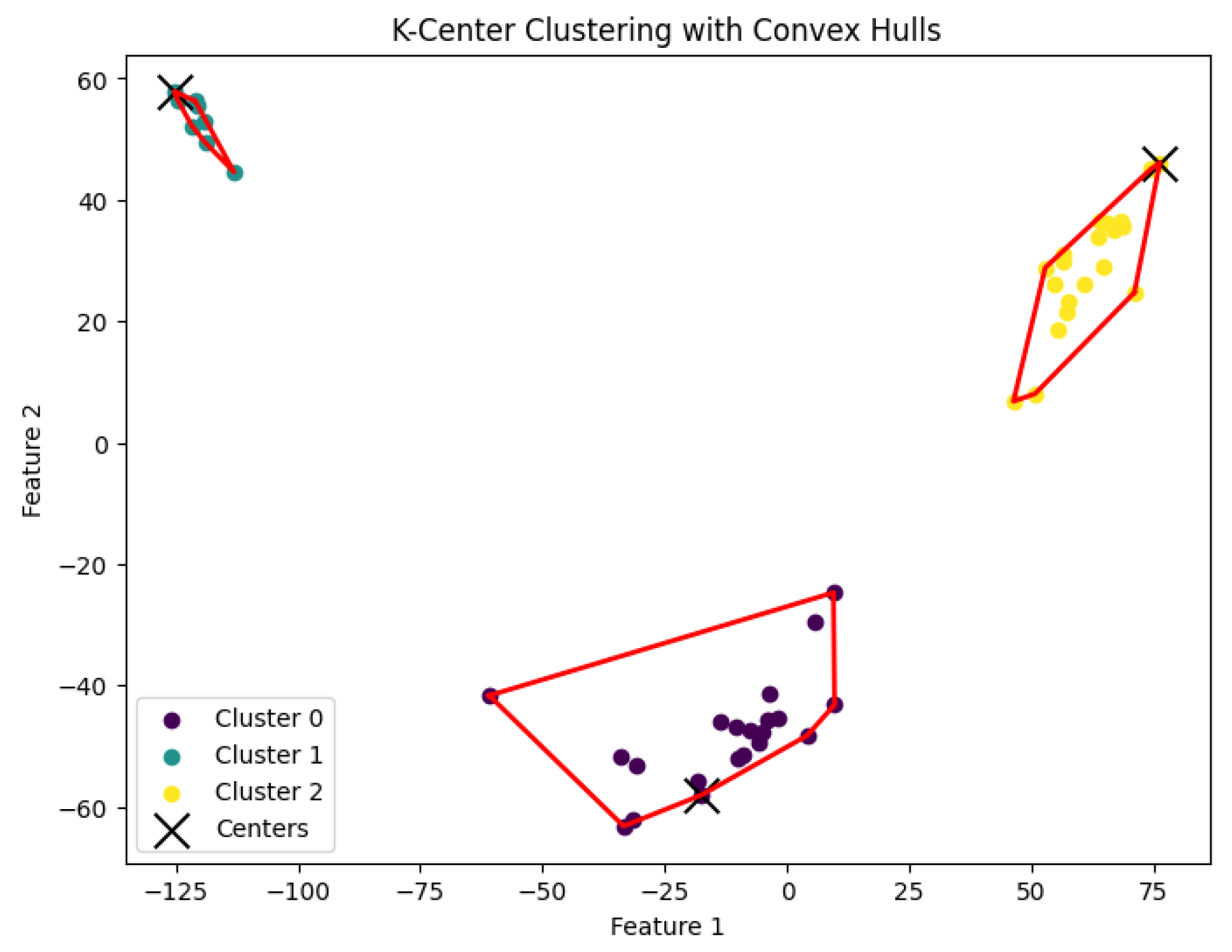
Figure 7.
The K-center clustering algorithm’s result with for the dataset Biase.
Figure 7.
The K-center clustering algorithm’s result with for the dataset Biase.
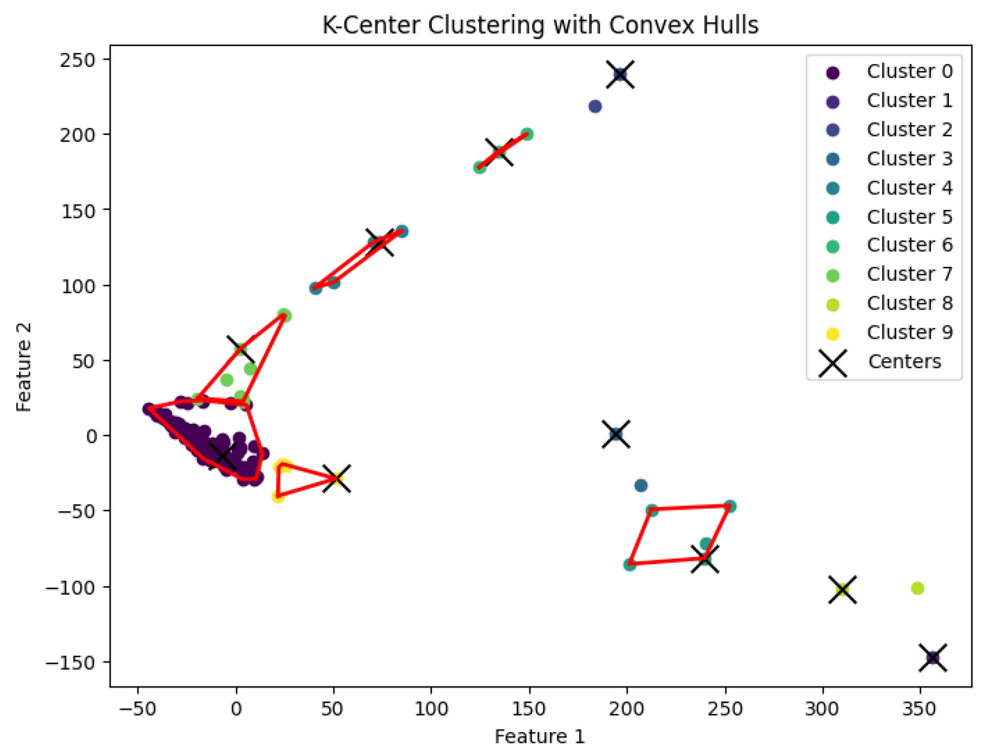
Figure 8.
The K-center clustering algorithm’s result with for the dataset Deng.
Figure 8.
The K-center clustering algorithm’s result with for the dataset Deng.
Figure 9.
The K-center clustering algorithm’s result with for the dataset Goolam.
Figure 9.
The K-center clustering algorithm’s result with for the dataset Goolam.
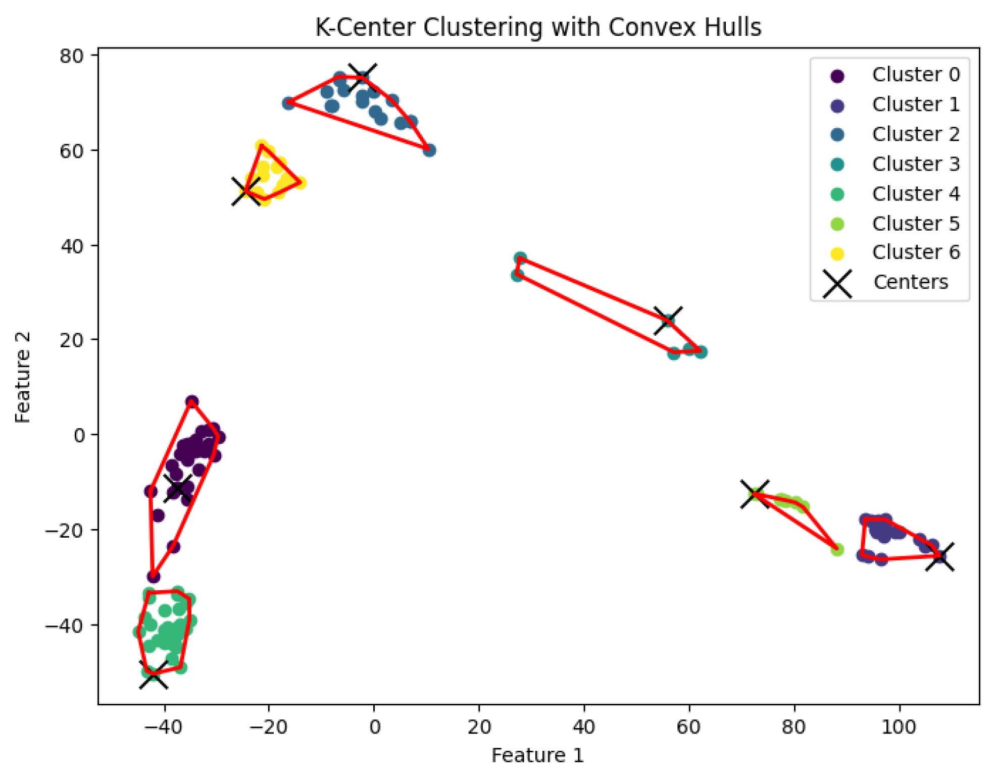
Figure 10.
The K-center clustering algorithm’s result with for the dataset Ting.
Figure 10.
The K-center clustering algorithm’s result with for the dataset Ting.
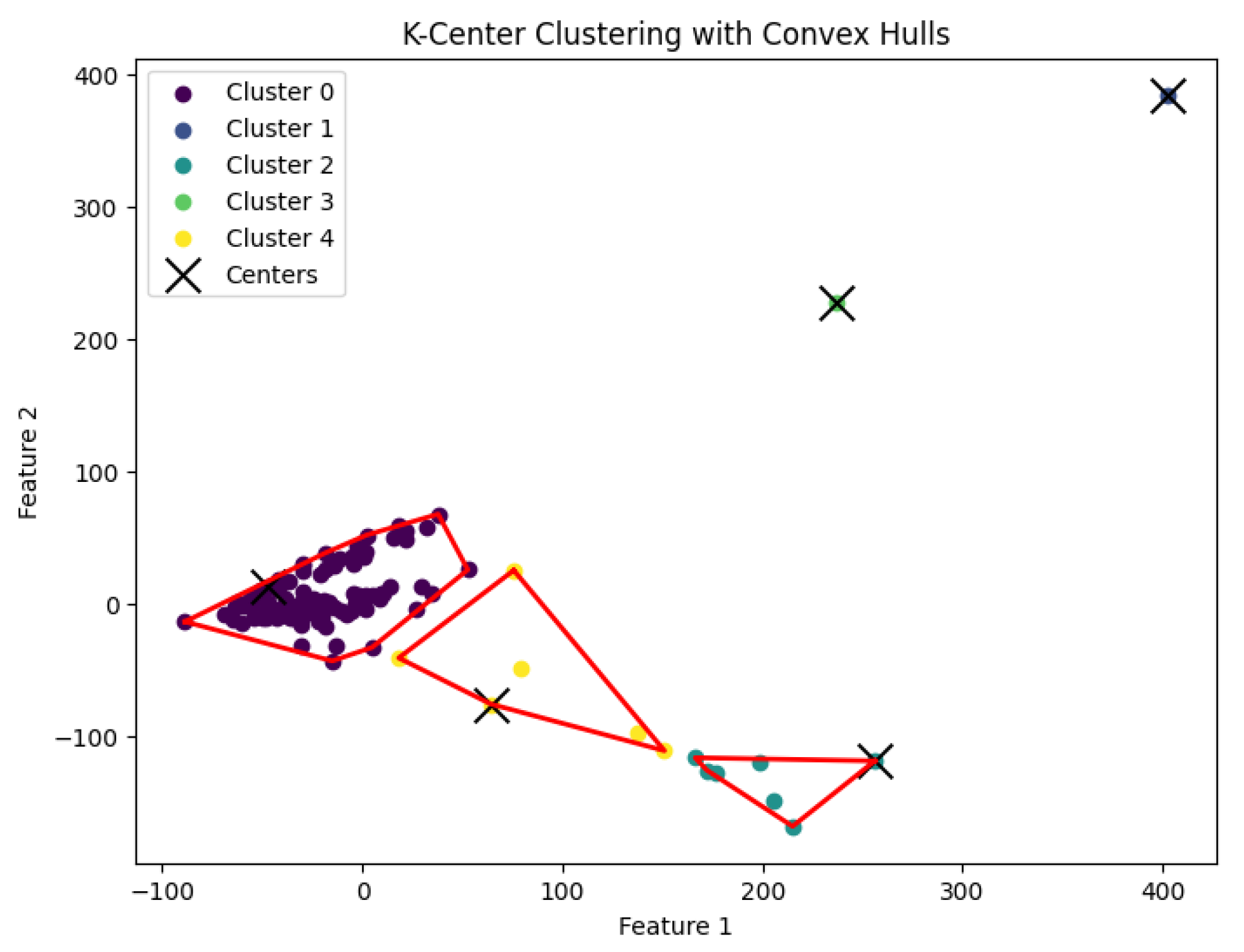
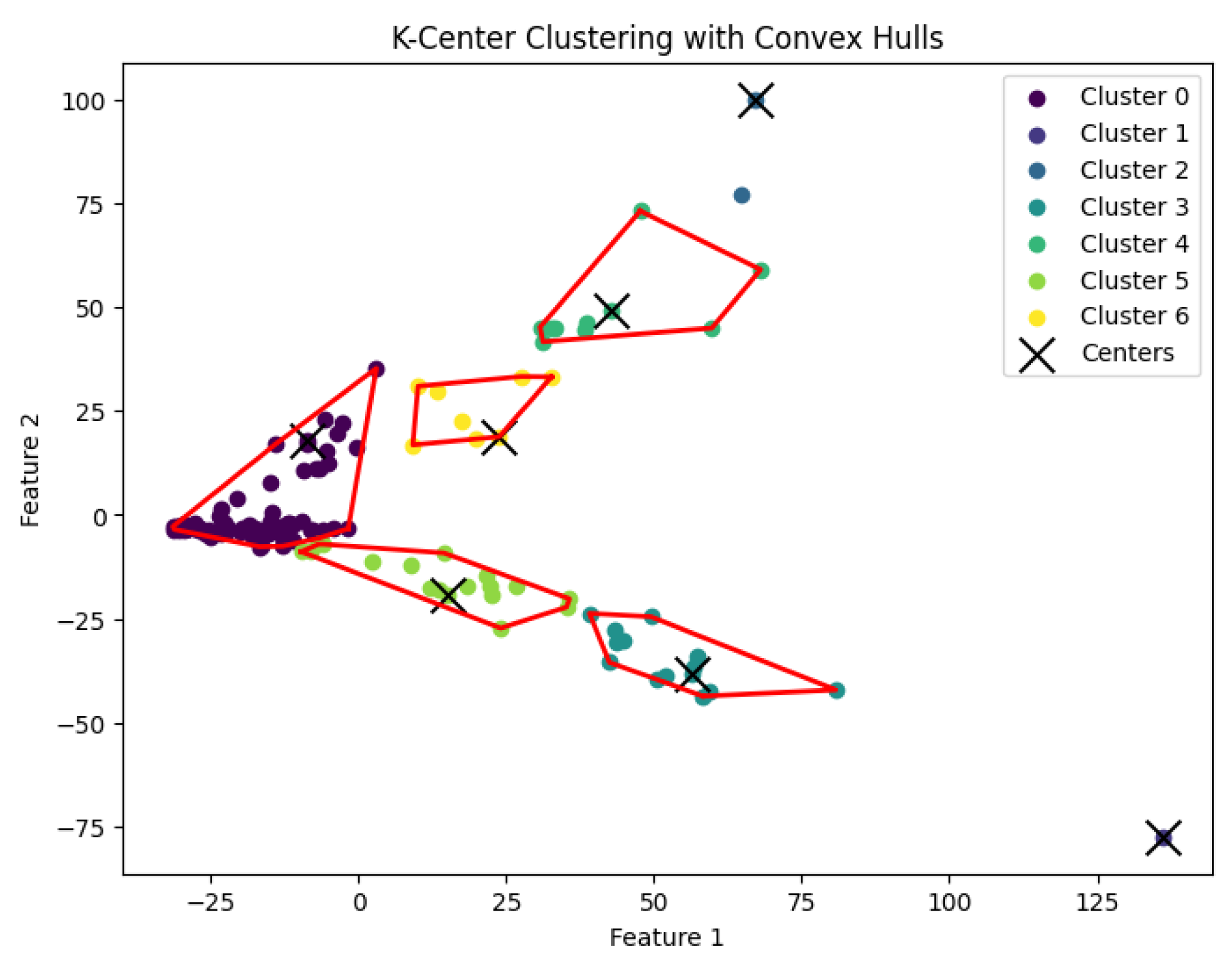
Figure 11.
The K-center clustering algorithm’s result with for the dataset Yan.
Figure 11.
The K-center clustering algorithm’s result with for the dataset Yan.
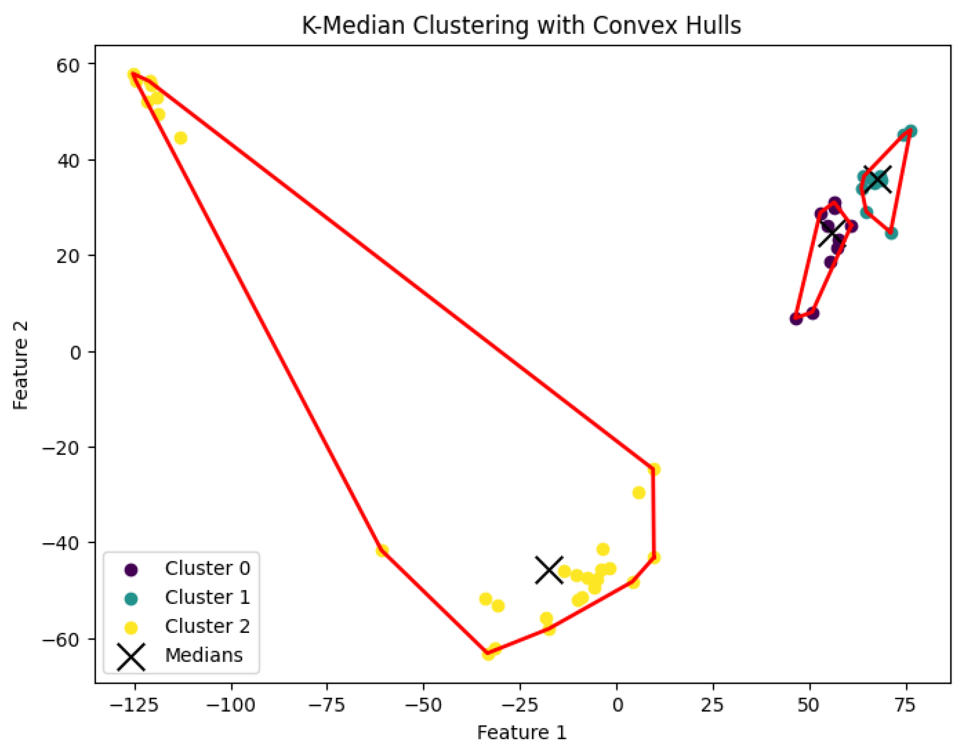
Figure 12.
The K-median clustering algorithm’s result with for the dataset Biase.
Figure 12.
The K-median clustering algorithm’s result with for the dataset Biase.
Figure 13.
The K-median clustering algorithm’s result with for the dataset Deng.
Figure 13.
The K-median clustering algorithm’s result with for the dataset Deng.
Figure 14.
The K-median clustering algorithm’s result with for the dataset Goolam.
Figure 14.
The K-median clustering algorithm’s result with for the dataset Goolam.
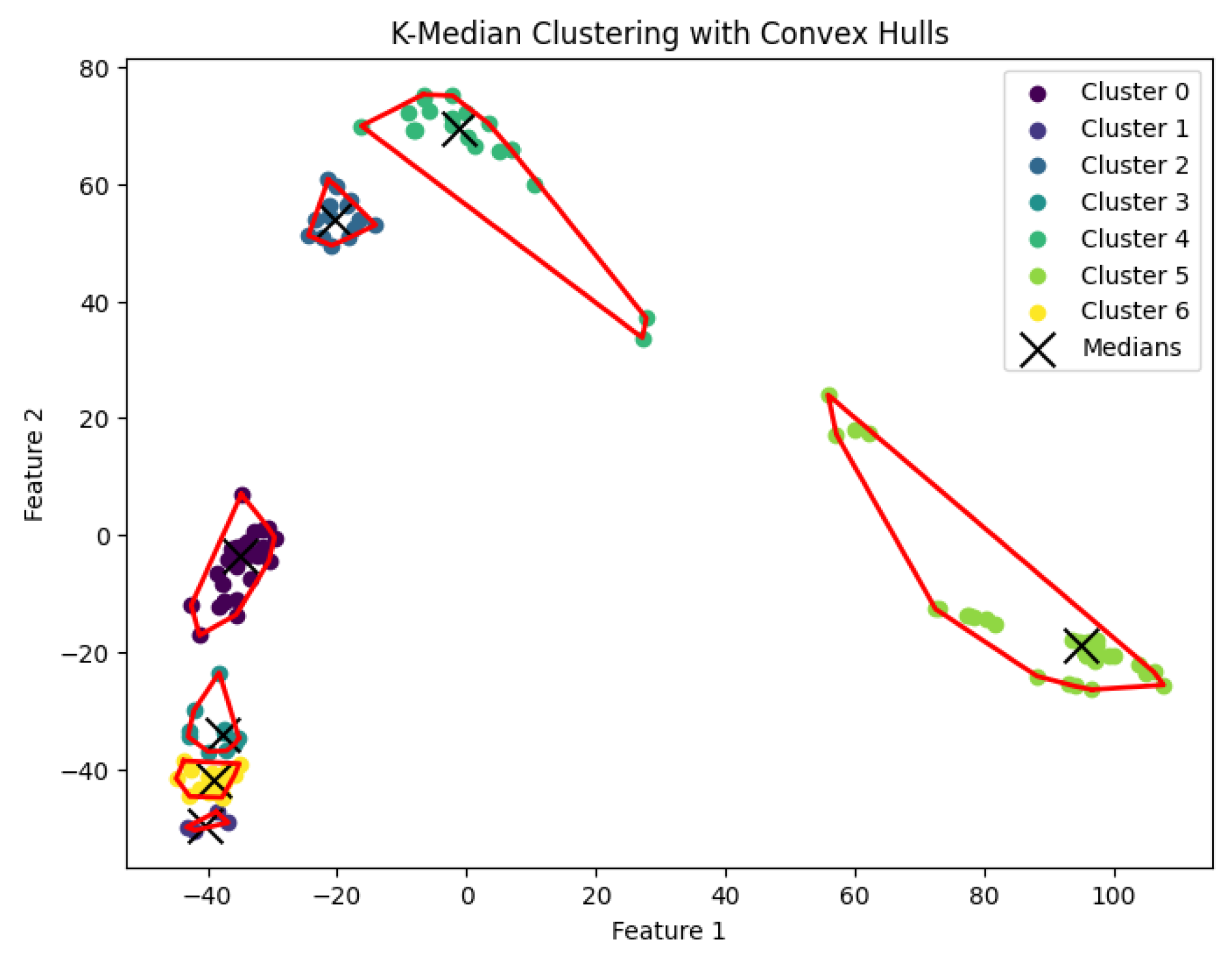
Figure 15.
The K-median clustering algorithm’s result with for the dataset Ting.
Figure 15.
The K-median clustering algorithm’s result with for the dataset Ting.
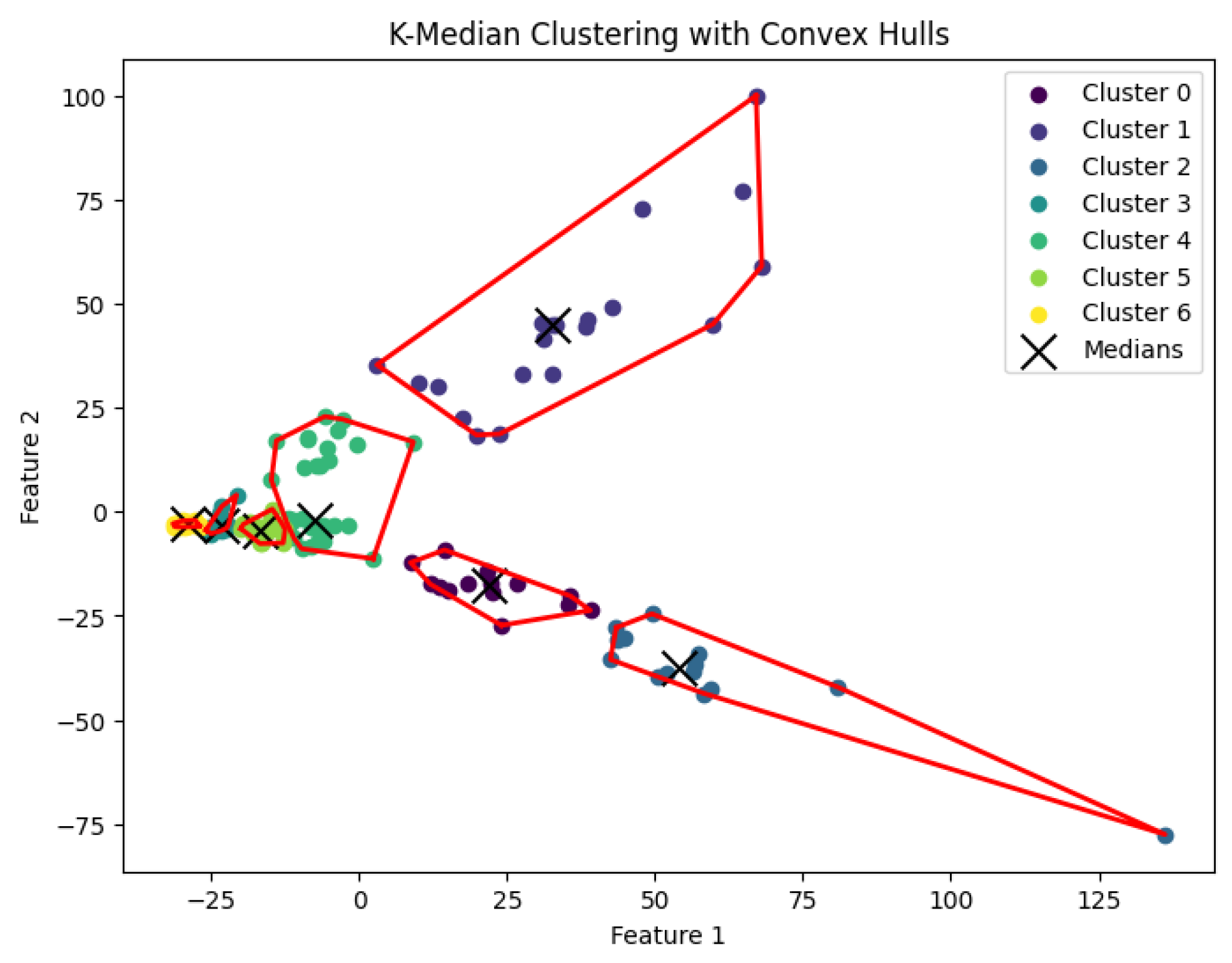
Figure 16.
The K-median clustering algorithm’s result with for the dataset Yan.
Figure 16.
The K-median clustering algorithm’s result with for the dataset Yan.
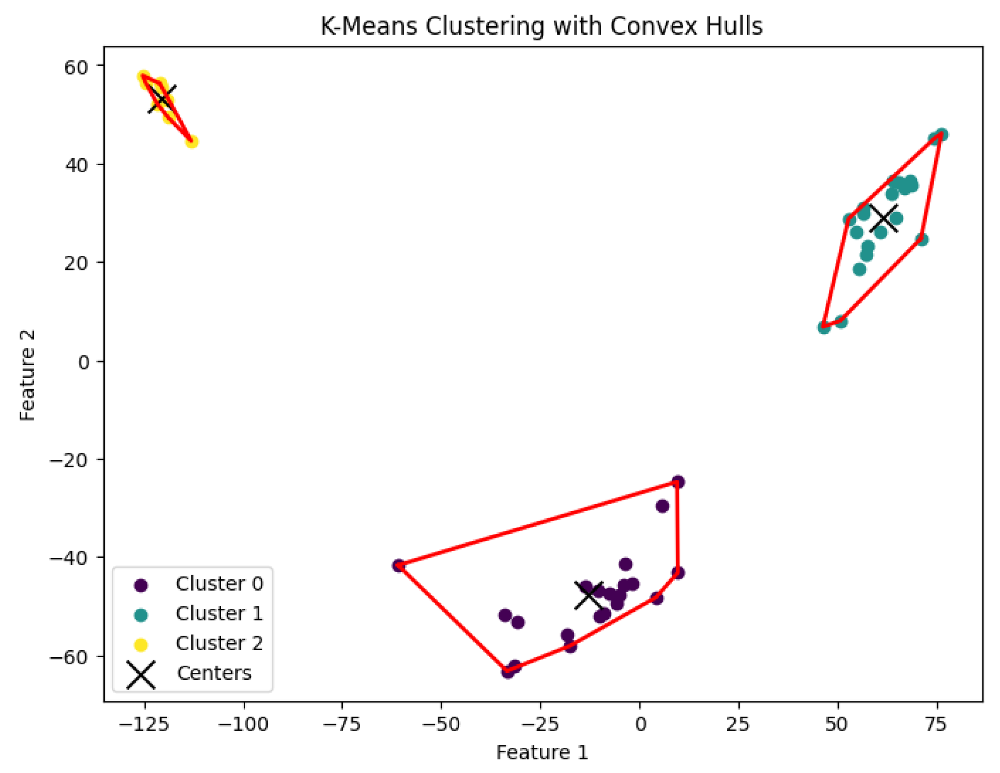
Figure 17.
The K-means clustering algorithm’s result with for the dataset Biase.
Figure 17.
The K-means clustering algorithm’s result with for the dataset Biase.
Figure 18.
The K-means clustering algorithm’s result with for the dataset Deng.
Figure 18.
The K-means clustering algorithm’s result with for the dataset Deng.
Figure 19.
The K-means clustering algorithm’s result with for the dataset Goolam.
Figure 19.
The K-means clustering algorithm’s result with for the dataset Goolam.
Figure 20.
The K-means clustering algorithm’s result with for the dataset Ting.
Figure 20.
The K-means clustering algorithm’s result with for the dataset Ting.
Figure 21.
The K-means clustering algorithm’s result with for the dataset Yan.
Figure 21.
The K-means clustering algorithm’s result with for the dataset Yan.
Figure 22.
The K-area clustering algorithm’s result with for the dataset Biase. The red dotted circle highlights an outlier.
Figure 22.
The K-area clustering algorithm’s result with for the dataset Biase. The red dotted circle highlights an outlier.
Figure 23.
The K-area clustering algorithm’s result with for the dataset Deng.
Figure 23.
The K-area clustering algorithm’s result with for the dataset Deng.
Figure 24.
The K-area clustering algorithm’s result with for the dataset Goolam.
Figure 24.
The K-area clustering algorithm’s result with for the dataset Goolam.
Figure 25.
The K-area clustering algorithm’s result with for the dataset Ting. MEF: mouse embryonic fibroblast; WBC: white blood cell; NB508: pancreatic cancer cell line; CTC: circulating tumor cell.
Figure 25.
The K-area clustering algorithm’s result with for the dataset Ting. MEF: mouse embryonic fibroblast; WBC: white blood cell; NB508: pancreatic cancer cell line; CTC: circulating tumor cell.
Figure 26.
The K-area clustering algorithm’s result with for the dataset Yan.
Figure 26.
The K-area clustering algorithm’s result with for the dataset Yan.
Figure 27.
Comparison of four clustering algorithms based on their performance, evaluated using NMI values.
Figure 27.
Comparison of four clustering algorithms based on their performance, evaluated using NMI values.
Figure 28.
Comparison of four clustering algorithms based on their performance, evaluated using convex area sizes.
Figure 28.
Comparison of four clustering algorithms based on their performance, evaluated using convex area sizes.
Figure 29.
The area ratios reveal the number of clusters needed.
Figure 29.
The area ratios reveal the number of clusters needed.
Figure 30.
One cluster for Yan.
Figure 30.
One cluster for Yan.
Figure 31.
Two clusters for Yan.
Figure 31.
Two clusters for Yan.
Figure 32.
Three clusters for Yan.
Figure 32.
Three clusters for Yan.
Figure 33.
Four clusters for Yan.
Figure 33.
Four clusters for Yan.
Figure 34.
Five clusters for Yan.
Figure 34.
Five clusters for Yan.
Figure 35.
Six clusters for Yan.
Figure 35.
Six clusters for Yan.
Figure 36.
Seven clusters for Yan.
Figure 36.
Seven clusters for Yan.
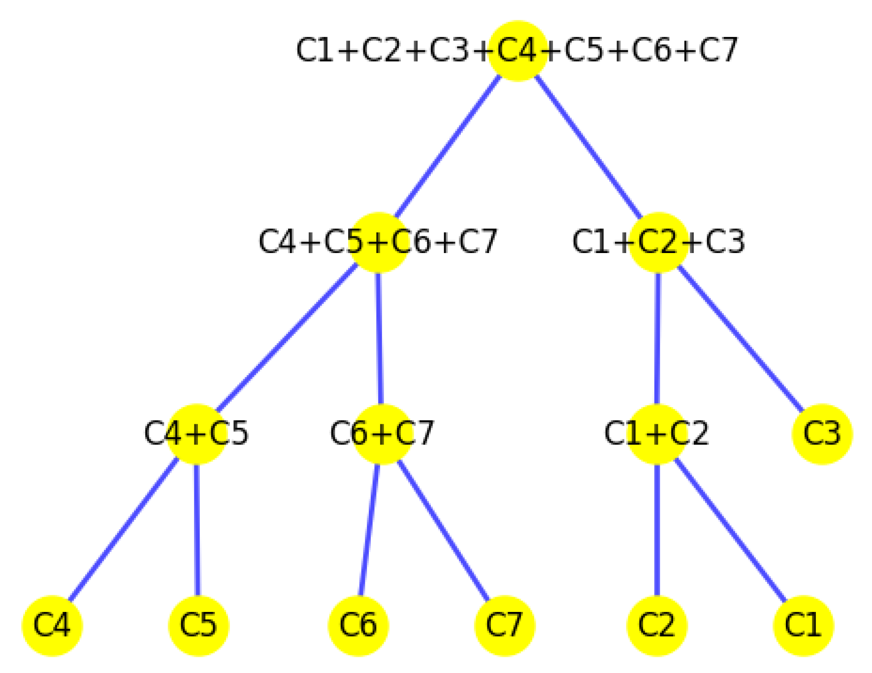
Figure 37.
The tree structure representing the partition made by the K-area algorithm.
Figure 37.
The tree structure representing the partition made by the K-area algorithm.
Table 1.
Different types of clustering algorithms. ∗: denotes our approach in this paper.
Table 1.
Different types of clustering algorithms. ∗: denotes our approach in this paper.
| Center-Based Clusters | High-Density Clusters | Center-Based Density Clusters ∗ |
|---|
| K-center clustering | K-median clustering | K-means clustering | K-high-density regions | K-volume clustering ∗ |
| NP-hard | NP-hard | NP-hard | NP-hard | - |
| An iterative greedy algorithm [4] | An iterative greedy algorithm [5] | An iterative greedy algorithm [24] | An iterative greedy algorithm [25] | An iterative greedy algorithm ∗ |
Table 2.
Datasets that we use for the experimental study of clustering algorithms.
Table 2.
Datasets that we use for the experimental study of clustering algorithms.
| Name | Size (# of Cells) | Size (# of Genes) | : # of Optimal Clusters | PubMed ID |
|---|
| Biase | 49 | 25,738 | 3 | 25096407 |
| Deng | 268 | 22,431 | 10 | 24408435 |
| Goolam | 124 | 41,480 | 5 | 27015307 |
| Ting | 149 | 29,018 | 7 | 25242334 |
| Yan | 90 | 20,214 | 7 | 23934149 |
Table 3.
Detailed NMI scores of four clustering algorithms. We use ∗ to denote the best results.
Table 3.
Detailed NMI scores of four clustering algorithms. We use ∗ to denote the best results.
| Dataset/Algorithms | K-Center | K-Median | K-Means | K-Area |
|---|
| Biase | | | | 0.533 ∗ |
| Deng | | 0.567 ∗ | | |
| Goolam | | | | 0.474 ∗ |
| Ting | | 0.544 ∗ | | |
| Yan | | | | 0.542 ∗ |
Table 4.
Comparison of four clustering algorithms’ running time (in seconds).
Table 4.
Comparison of four clustering algorithms’ running time (in seconds).
| Dataset/Algorithms | K-Center | K-Median | K-Means | K-Area |
|---|
| Biase | 23 | 20 | 21 | 5 |
| Deng | 26 | 25 | 28 | 641 |
| Goolam | 20 | 23 | 22 | 59 |
| Ting | 19 | 20 | 22 | 66 |
| Yan | 14 | 14 | 19 | 50 |
Table 5.
Detailed convex area sizes of four clustering algorithms.
Table 5.
Detailed convex area sizes of four clustering algorithms.
| Dataset/Algorithms | K-Center | K-Median | K-Means | K-Area |
|---|
| Biase | | | | |
| Deng | | 13,640.09 | | |
| Goolam | 17,083.75 | 28,588.06 | 15,519.73 | 11,270.08 |
| Ting | | | 11,114.86 | |
| Yan | | | | |
Table 6.
The total clusters’ area and the ratios of the convex hull areas between two neighboring rounds help determine the value K.
Table 6.
The total clusters’ area and the ratios of the convex hull areas between two neighboring rounds help determine the value K.
| # of Total Cluster | Total Convex Hull’s Area | Area Ratios of Two Neighboring Rounds |
|---|
| 1 | 10,530.41 | 0 |
| 2 | 3110.62 | 0.30 |
| 3 | 2271.75 | 0.73 |
| 4 | 1613.22 | 0.71 |
| 5 | 1167.92 | 0.72 |
| 6 | 956.11 | 0.82 |
| 7 | 770.70 | 0.81 |
| 8 | 654.54 | 0.85 |
| 9 | 590.55 | 0.90 |


