
Support Vector Machine-Based Classification of Vasovagal Syncope Using Head-Up Tilt Test


Abstract
:Simple Summary
Abstract
1. Introduction
2. Related Work
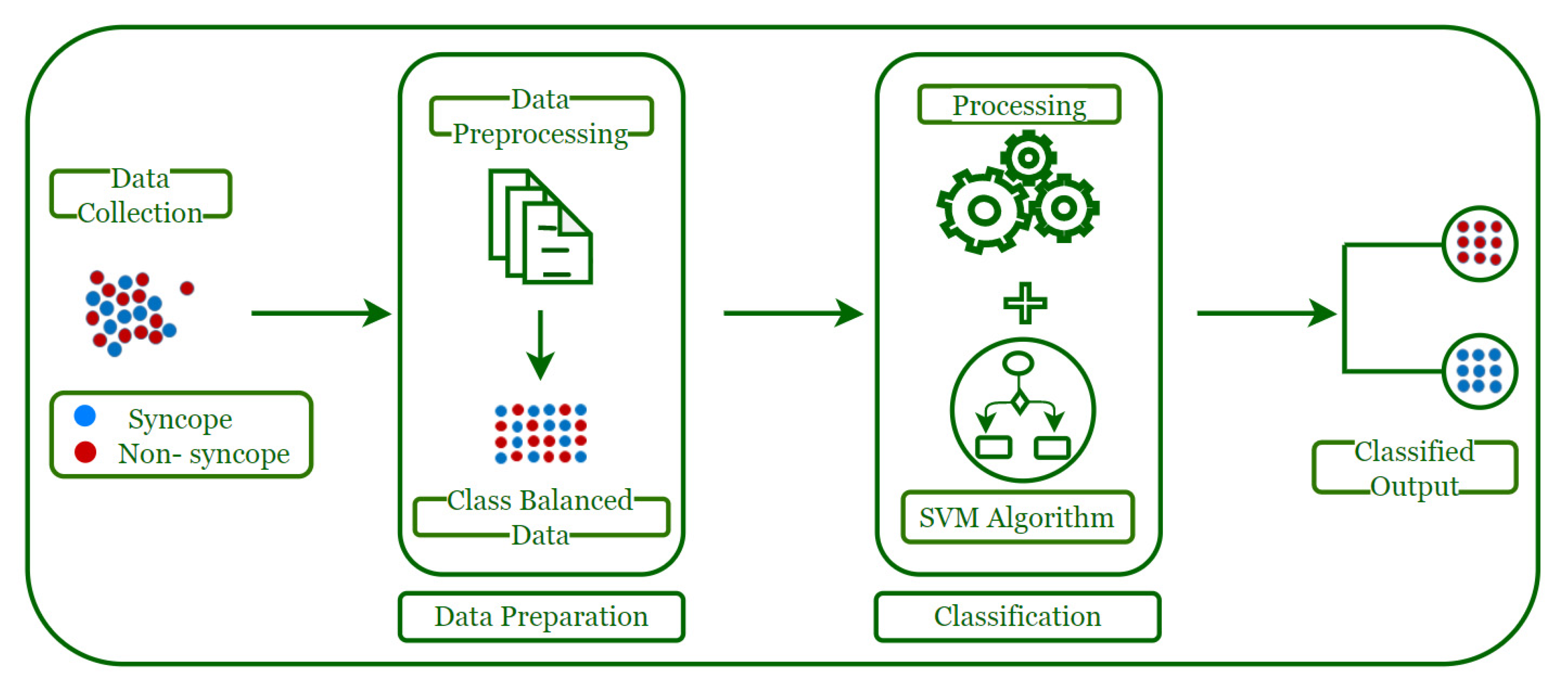
3. Syncope Classification Model
3.1. Data Collection
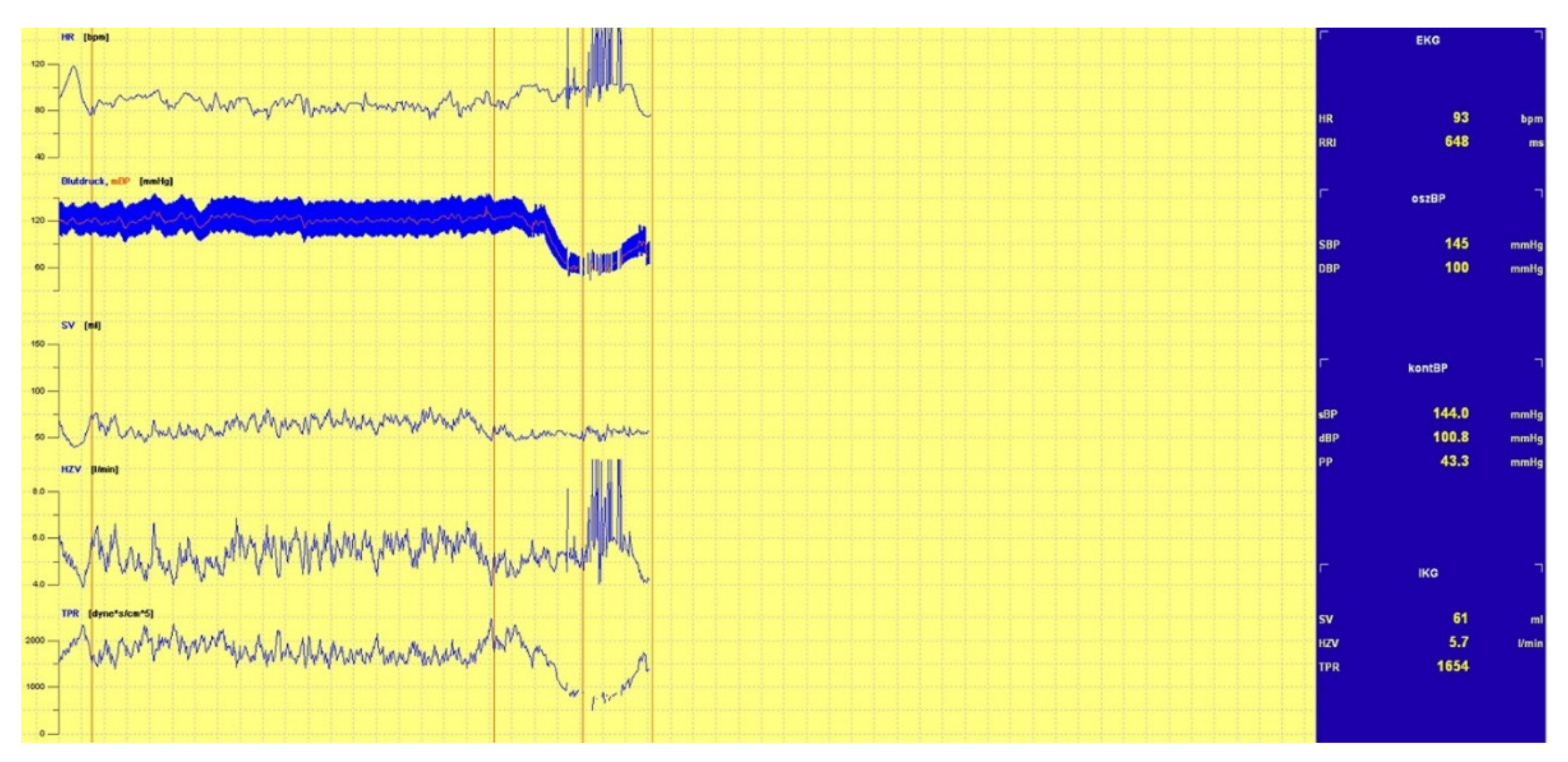
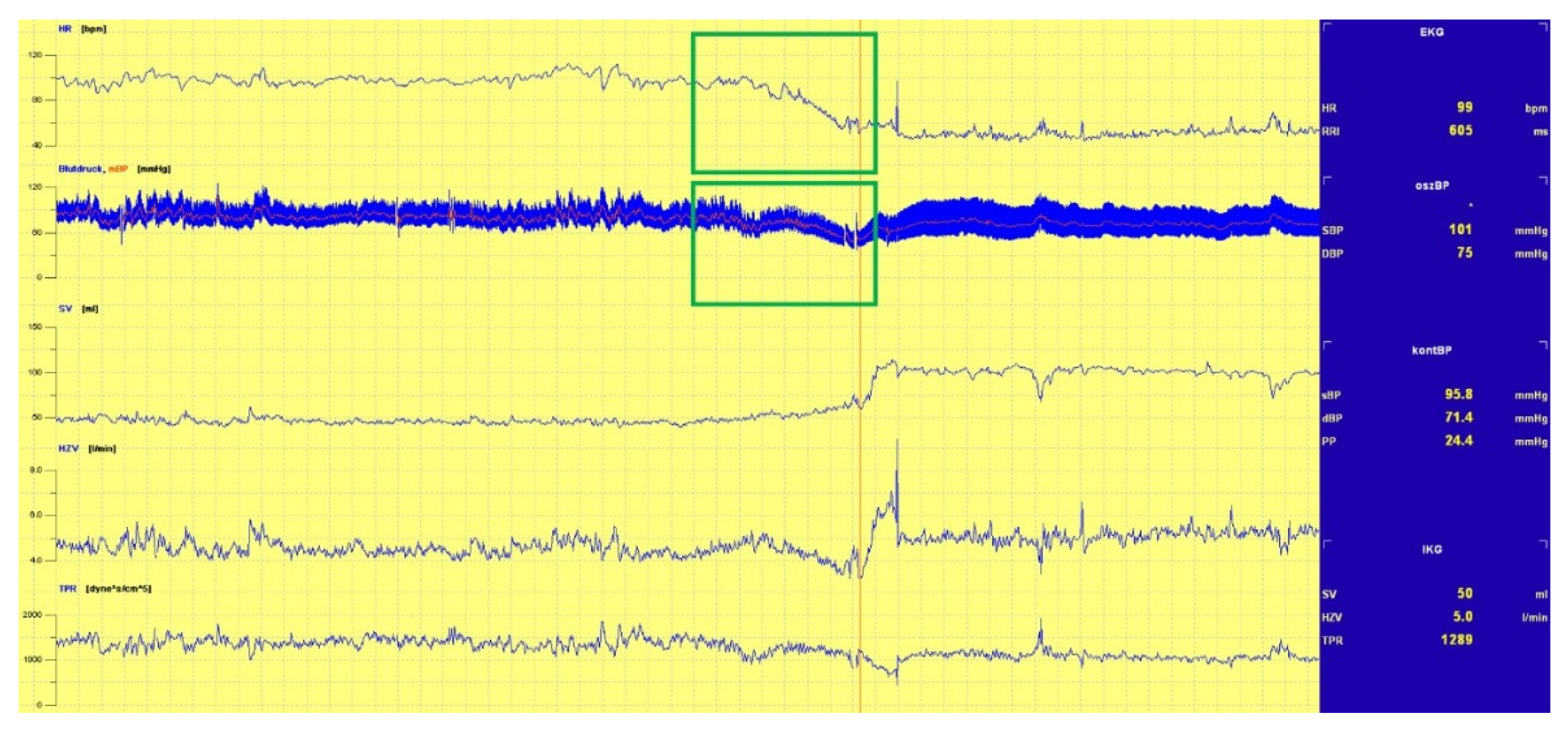
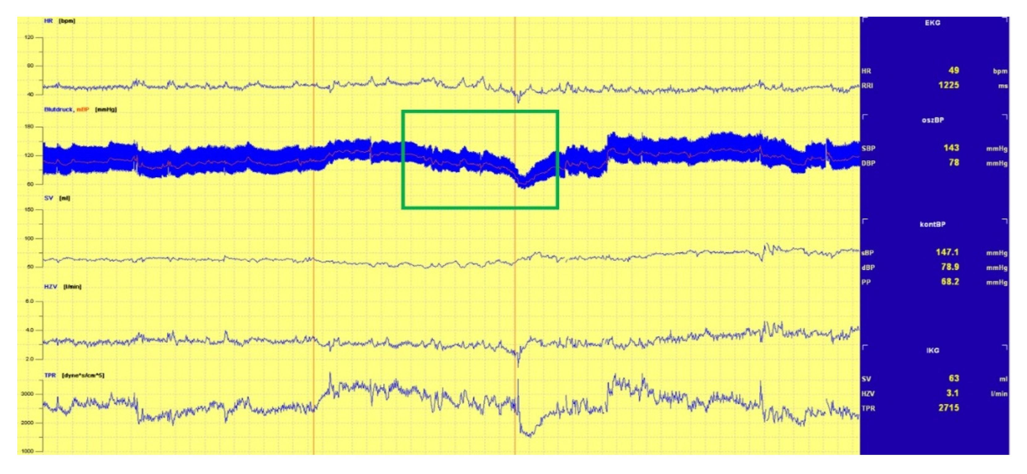
3.1.1. Head-Up Tilt (HUT) Test
3.1.2. Data Organization
3.2. Data Preparation
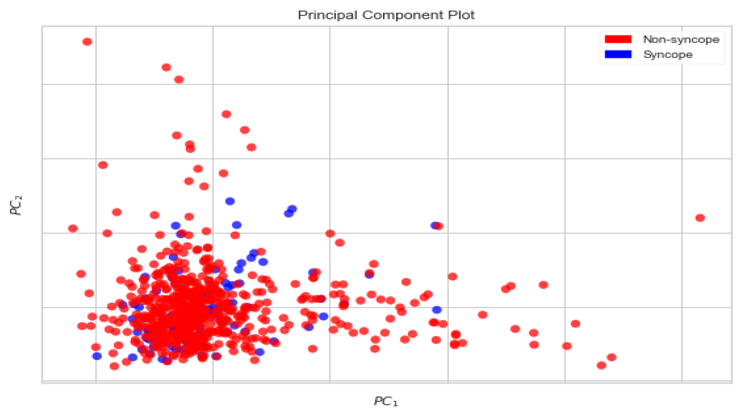
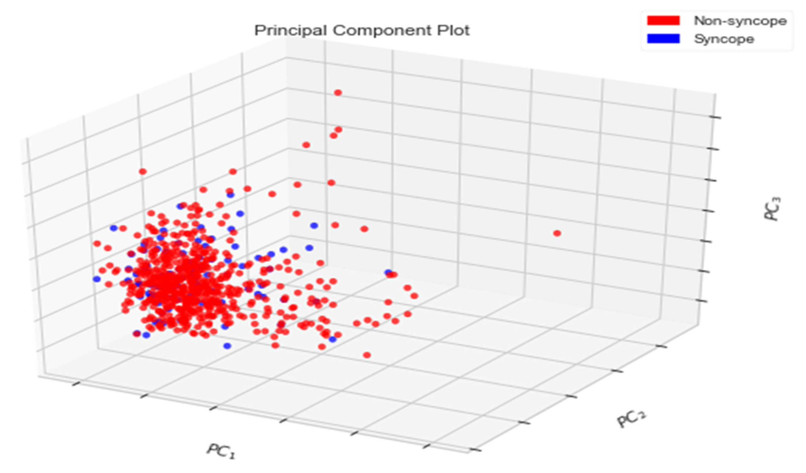
Principal Components Analysis
3.3. Data Classification
3.3.1. Support Vector Machine
= 2/||w||
3.3.2. Performance Metrics
3.4. Classified Output
- The imbalance in classes of data has not been addressed;
- The generated dataset is based on responses to a questionnaire instead of the true physiological data;
- The generated dataset is based on the observations made by individual physicians and not on continuous observation of the heart rate and beat-to-beat recording of blood pressure.
3.4.1. Contributing Features
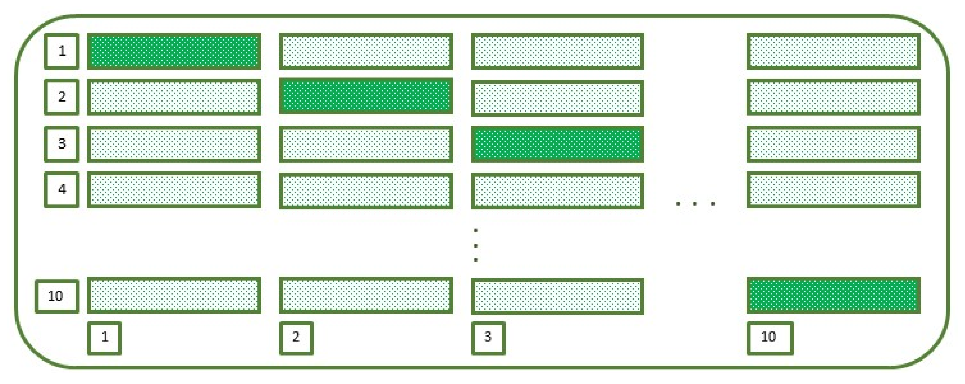
3.4.2. Train–Test–Split Evaluation
3.4.3. K-Fold Cross-Validation Evaluation
4. Limitations and Future Work
5. Conclusions
Author Contributions
Funding
Institutional Review Board Statement
Informed Consent Statement
Data Availability Statement
Conflicts of Interest
References
- Brignole, M. ‘Ten Commandments’ of ESC syncope guidelines 2018: The new European Society of Cardiology (ESC) clinical practice guidelines for the diagnosis and management of syncope were launched 19 March 2018 at EHRA 2018 in Barcelona. Eur. Heart J. 2018, 39, 1870–1871. [Google Scholar] [CrossRef] [PubMed]
- Brignole, M.; Moya, A.; De Lange, F.J.; Deharo, J.-C.; Elliott, P.M.; Fanciulli, A.; Fedorowski, A.; Furlan, R.; Kenny, R.A.; Martínez, A.M.; et al. Practical Instructions for the 2018 ESC Guidelines for the diagnosis and management of syncope. Eur. Heart J. 2018, 39, e43–e80. [Google Scholar] [CrossRef] [PubMed]
- Puppala, V.K.; Dickinson, O.; Benditt, D.G. Syncope: Classification and risk stratification. J. Cardiol. 2014, 63, 171–177. [Google Scholar] [CrossRef] [PubMed] [Green Version]
- Sutton, R. Clinical classification of syncope. Prog. Cardiovasc. Dis. 2013, 55, 339–344. [Google Scholar] [CrossRef] [PubMed]
- Dolley, S. Big data’s role in precision public health. Front. Public Health 2018, 6, 68. [Google Scholar] [CrossRef]
- Jayaraman, P.P.; Forkan AR, M.; Morshed, A.; Haghighi, P.D.; Kang, Y.B. Healthcare 4.0: A review of frontiers in digital health. Wiley Interdiscip. Rev. Data Min. Knowl. Discov. 2020, 10, e1350. [Google Scholar] [CrossRef]
- Thanavaro, J.L. Evaluation and Management of Syncope. Clin. Sch. Rev. 2009, 2, 65–77. [Google Scholar] [CrossRef]
- Callahan, A.; Shah, N.H. Machine learning in healthcare. In Key Advances in Clinical Informatics; Academic Press: Cambridge, MA, USA, 2017; pp. 279–291. [Google Scholar]
- Dhillon, A.; Singh, A. Machine learning in healthcare data analysis: A survey. J. Biol. Todays World 2019, 8, 1–10. [Google Scholar]
- Hart, J.; Mehlsen, J.; Olsen, C.H.; Olufsen, M.S.; Gremaud, P. Classification of syncope through data analytics. arXiv 2016, arXiv:1609.02049. [Google Scholar]
- Brignole, M. Diagnosis and treatment of syncope. Heart 2007, 93, 130–136. [Google Scholar] [CrossRef] [PubMed] [Green Version]
- Mehlsen, J.; Kaijer, M.N.; Mehlsen, A.-B. Autonomic and electrocardiographic changes in cardioinhibitory syncope. Europace 2008, 10, 91–95. [Google Scholar] [CrossRef]
- Moya, A.; Sutton, R.; Ammirati, F.; Blanc, J.-J.; Brignole, M.; Dahm, J.B.; Deharo, J.-C.; Gajek, J.; Gjesdal, K.; The Task Force for the Diagnosis and Management of Syncope of the European Society of Cardiology (ESC); et al. Guidelines for the diagnosis and management of syncope (version 2009). Eur. Heart J. 2009, 30, 2631–2671. [Google Scholar] [CrossRef] [Green Version]
- Van Dijk, J.G.; Thijs, R.D.; Benditt, D.G.; Wieling, W. A guide to disorders causing transient loss of consciousness: Focus on syncope. Nat. Rev. Neurol. 2009, 5, 438–448. [Google Scholar] [CrossRef] [PubMed]
- Wardrope, A.; Jamnadas-Khoda, J.; Broadhurst, M.; Grünewald, R.A.; Heaton, T.J.; Howell, S.J.; Koepp, M.; Parry, S.W.; Sisodiya, S.; Walker, M.C.; et al. Machine learning as a diagnostic decision aid for patients with transient loss of consciousness. Neurol. Clin. Pract. 2020, 10, 96–105. [Google Scholar] [CrossRef] [PubMed]
- Khodor, N.; Carrault, G.; Matelot, D.; Amoud, H.; Khalil, M.; du Boullay, N.T.; Carre, F.; Hernández, A. Early syncope detection during head up tilt test by analyzing interactions between cardio-vascular signals. Digit. Signal Process. 2016, 49, 86–94. [Google Scholar] [CrossRef]
- Parry, S.W.; Kenny, R.A. Tilt table testing in the diagnosis of unexplained syncope. QJM 1999, 92, 623–629. [Google Scholar] [CrossRef] [Green Version]
- Goswami, N.; Lackner, H.; Grasser, E.K.; Hinghofer-Szalkay, H.G. Individual stability of orthostatic tolerance response. Acta Physiol. Hung. 2009, 96, 157–166. [Google Scholar] [CrossRef]
- Goswami, N.; Roessler, A.; Lackner, H.K.; Schneditz, D.; Grasser, E.; Hinghofer-Szalkay, H.G. Heart rate and stroke volume response patterns to augmented orthostatic stress. Clin. Auton. Res. 2009, 19, 157–165. [Google Scholar] [CrossRef] [PubMed]
- Trozic, I.; Platzer, D.; Fazekas, F.; Bondarenko, A.I.; Brix, B.; Rössler, A.; Goswami, N. Postural hemodynamic parameters in older persons have a seasonal dependency. Z. Für Gerontol. Und Geriatr. 2020, 53, 145–155. [Google Scholar] [CrossRef] [Green Version]
- Dorogovtsev, V.; Yankevich, D.; Goswami, N. Effects of an Innovative Head-Up Tilt Protocol on Blood Pressure and Arterial Stiffness Changes. J. Clin. Med. 2021, 10, 1198. [Google Scholar] [CrossRef]
- Goswami, N.; Singh, A.; Deepak, K.K. Developing a “dry lab” activity using lower body negative pressure to teach physiology. Adv. Physiol. Educ. 2021, 45, 445–453. [Google Scholar] [CrossRef] [PubMed]
- Laing, C.; Green, D.A.; Mulder, E.; Hinghofer-Szalkay, H.; Blaber, A.P.; Rittweger, J.; Goswami, N. Effect of novel short-arm human centrifugation-induced gravitational gradients upon cardiovascular responses, cerebral perfusion and g-tolerance. J. Physiol. 2020, 598, 4237–4249. [Google Scholar] [CrossRef] [PubMed]
- Goswami, N.; Blaber, A.P.; Hinghofer-Szalkay, H.; Montani, J.-P. Orthostatic Intolerance in Older Persons: Etiology and Countermeasures. Front. Physiol. 2017, 8, 803. [Google Scholar] [CrossRef] [PubMed] [Green Version]
- Winter, J.; Laing, C.; Johannes, B.; Mulder, E.; Brix, B.; Roessler, A.; Reichmuth, J.; Rittweger, J.; Goswami, N. Galanin and Adrenomedullin Plasma Responses During Artificial Gravity on a Human Short-Arm Centrifuge. Front. Physiol. 2019, 9, 1956. [Google Scholar] [CrossRef] [PubMed]
- Chawla, N.V.; Bowyer, K.; Hall, L.O.; Kegelmeyer, W.P. SMOTE: Synthetic Minority Over-sampling Technique. J. Artif. Intell. Res. 2002, 16, 321–357. [Google Scholar] [CrossRef]
- He, H.; Bai, Y.; Garcia, E.A.; Li, S. ADASYN: Adaptive synthetic sampling approach for imbalanced learning. In Proceedings of the IEEE International Joint Conference on Neural Networks, IEEE World Congress on Computational Intelligence, Hong Kong, China, 1–8 June 2008. [Google Scholar]
- Arozi, M.; Caesarendra, W.; Ariyanto, M.; Munadi, M.; Setiawan, J.D.; Glowacz, A. Pattern Recognition of Single-Channel sEMG Signal Using PCA and ANN Method to Classify Nine Hand Movements. Symmetry 2020, 12, 541. [Google Scholar] [CrossRef] [Green Version]
- Weston, J.; Watkins, C. Support vector machines for multi-class pattern recognition. In Proceedings of the ESANN—European Symposium on Artificial Neural Networks, Bruges, Belgium, 21–23 April 1999; Volume 99, pp. 219–224. [Google Scholar]
- Luque, A.; Carrasco, A.; Martín, A.; Heras, A.D.L. The impact of class imbalance in classification performance metrics based on the binary confusion matrix. Pattern Recognit. 2019, 91, 216–231. [Google Scholar] [CrossRef]
- Goutte, C.; Gaussier, E. A probabilistic interpretation of precision recall and F-score, with implication for evaluation. In European Conference on Information Retrieval; Springer: Berlin/Heidelberg, Germany, 2005; pp. 345–359. [Google Scholar]
- Metz, C.E. Basic principles of ROC analysis. Semin. Nucl. Med. 1978, 8, 283–298. [Google Scholar] [CrossRef]
- Duda, R.O.; Hart, P.E. Pattern Classification and Scene Analysis; Wiley: New York, NY, USA, 1973; Volume 3, pp. 731–739. [Google Scholar]
- Bottou, L. Stochastic gradient descent tricks. In Neural Networks: Tricks of the Trade; Springer: Berlin/Heidelberg, Germany, 2012; pp. 421–436. [Google Scholar]
- Rodriguez, J.; Blaber, A.P.; Kneihsl, M.; Trozic, I.; Ruedl, R.; Green, D.A.; Broadbent, J.; Xu, D.; Rössler, A.; Hinghofer-Szalkay, H.; et al. Poststroke alterations in heart rate variability during orthostatic challenge. Medicine 2017, 96, e5989. [Google Scholar] [CrossRef] [Green Version]
- Blain, H.; Masud, T.; Dargent-Molina, P.; Martin, F.C.; Rosendahl, E.; van der Velde, N.; Bousquet, J.; Benetos, A.; Cooper, C.; Kanis, J.A.; et al. A comprehensive fracture prevention strategy in older adults: The European Union Geriatric Medicine Society (EUGMS) statement. J. Nutr. Health Aging 2016, 20, 647–652. [Google Scholar] [CrossRef] [Green Version]
- Bousquet, J.; Bewick, M.; Cano, A.; Eklund, P.; Fico, G.; Goswami, N.; Guldemond, N.A.; Henderson, D.; Hinkema, M.J.; Liotta, G.; et al. Building bridges for innovation in ageing: Synergies between action groups of the EIP on AHA. J. Nutr. Health Aging 2017, 21, 92–104. [Google Scholar] [CrossRef] [PubMed] [Green Version]
- Goswami, N. Falls and fall-prevention in older persons: Geriatrics meets spaceflight! Front. Physiol. 2017, 8, 603. [Google Scholar] [CrossRef] [PubMed] [Green Version]
- Batzel, J.J.; Goswami, N.; Lackner, H.K.; Roessler, A.; Bachar, M.; Kappel, F.; Hinghofer-Szalkay, H. Patterns of Cardiovascular Control During Repeated Tests of Orthostatic Loading. Cardiovasc. Eng. 2009, 9, 134–143. [Google Scholar] [CrossRef]
- Evans, J.M.; Knapp, C.F.; Goswami, N. Artificial Gravity as a Countermeasure to the Cardiovascular Deconditioning of Spaceflight: Gender Perspectives. Front. Physiol. 2018, 9, 716. [Google Scholar] [CrossRef] [PubMed]
- Patel, K.; Rössler, A.; Lackner, H.K.; Trozic, I.; Laing, C.; Lorr, D.; Green, D.A.; Hinghofer-Szalkay, H.; Goswami, N. Effect of postural changes on cardiovascular parameters across gender. Medicine 2016, 95, e4149. [Google Scholar] [CrossRef] [PubMed]
- Sachse, C.; Trozic, I.; Brix, B.; Roessler, A.; Goswami, N. Sex differences in cardiovascular responses to orthostatic challenge in healthy older persons: A pilot study. Physiol. Int. 2019, 106, 236–249. [Google Scholar] [CrossRef]
- Goswami, N.; Abulafia, C.; Vigo, D.; Moser, M.; Cornelissen, G.; Cardinali, D. Falls Risk, Circadian Rhythms and Melatonin: Current Perspectives. Clin. Interv. Aging 2020, 15, 2165–2174. [Google Scholar] [CrossRef]


| Age Group | Gender | Numbers | Age Group | Gender | Numbers |
|---|---|---|---|---|---|
| 0–15 | M | 01 | 55–65 | M | 07 |
| F | 02 | F | 13 | ||
| 15–25 | M | 01 | 65–75 | M | 14 |
| F | 04 | F | 09 | ||
| 25–35 | M | 02 | 75–85 | M | 03 |
| F | 02 | F | 11 | ||
| 35–45 | M | 06 | 85–95 | M | 02 |
| F | 03 | F | 01 | ||
| 45–55 | M | 07 | Total | M | 43 |
| F | 08 | F | 53 |
| Beatstats | |||
|---|---|---|---|
| Acronym | Definition | Equations | Units |
| HR | Heart Rate | Primitive | Beats/ min |
| SV | Stroke Volume | Primitive | Litre/beat |
| CO | Cardiac Output | SV[l/beat] × HR[bpm] | Litre/min |
| CI | Cardiac Input | CO[l/min]/Body Surface Area[m2] | Litre/min/m2 |
| SI | Stroke Index | SV[l/beat]/Body Surface Area[m2] × 1000 | Ml/beat/m2 |
| RRI | RR-Interval | Primitive | Seconds |
| TPR | Total Peripheral Resistance | Primitive | Pa·sec/m3 |
| TPRI | Total Peripheral Resistance Index | Primitive | Pa·sec/m5 |
| dBP | Diastolic Blood Pressure | Primitive | mmHg |
| mBp | Mean Blood Pressure | (2/3) × dBP[mmHg] + (1/3) × sBP[mmHg] | mmHg |
| sBP | Systolic Blood Pressure | Primitive | mmHg |
| Cardiacbeatstats | |||
| ACI | Acceleration Index | Primitive | m/s2 |
| CI | Cardiac Input | CO[l/min]/Body Surface Area[m2] | Litre/min/m2 |
| EDI | End-Diastolic Index | Primitive | |
| HR | Heart Rate | Primitive | Beats/ min |
| IC | Index of Contractility | Primitive | Seconds |
| LVET | Left VentricularPrimitiveEjection Time | Primitive | Milliseconds |
| LVWI | Left Ventricular Stroke Work Index | SI[ml/beat/m2] × (LVSP[mmHg]—LVEDP[mmHg]). | Pa.ml/beat/m2 |
| SI | Stroke Index | SV[l/beat]/Body Surface Area[m2] × 1000 | Ml/beat/m2 |
| TFC | Thoracic Fluid Content | Primitive | Litre |
| TPRI | Total Peripheral Resistance Index | Primitive | Pa·sec/m5 |
| dBP | Diastolic Blood Pressure | Primitive | mmHg |
| mBp | Mean Blood Pressure | (2/3) × dBP[mmHg] + (1/3) × sBP[mmHg] | mmHg |
| sBP | Systolic Blood Pressure | Primitive | mmHg |
| HRVstats | |||
| HF_RRI | High-Frequency RR Interval | Primitive | Hz |
| HFnu_RRI | Normalized High-Frequency RR Interval | HF_RRI/(HF_RRI + LF_RRI + VLF_RRI) | |
| LF_HF | Difference Between Low and High Frequency of RR Interval | HF_RRI ~ LF_RRI | Hz |
| LF_HF_RRI | The ratio of Low and High Frequency of RR Interval | LF_RRI/HF_RRI | |
| LF_RRI | Low-Frequency RR Interval | Primitive | Hz |
| LFnu_RRI | Normalized Low-Frequency RR Interval | LF_RRI/(HF_RRI +LF_RRI + VLF_RRI) | |
| PSD_RRI | Power Spectral Density of RR Interval | Primitive | W/Hz |
| VLF_RRI | Very Low Frequency of RR Interval | Primitive | Hz |
| dBPVstats | |||
| HF_dBP | High-Frequency dBP | Primitive | Hz |
| HFnu_dBP | Normalised High-Frequency dBP | HF_dBP/(HF_dBP+ LF_dBP + VLF_dBP) | |
| LF_HF | Difference Between Low and High Frequency of dBP | HF_dBP ~ LF_dBP | Hz |
| LF_HF_dBP | Ratio of Low and High Frequency of dBP | LF_dBP/HF_dBP | |
| LF_dBP | Low-Frequency dBP | Primitive | Hz |
| LFnu_dBP | Normalised Low-Frequency dBP | LF_dBP/(HF_dBP + LF_dBP + VLF_dBP) | |
| PSD_dBP | Power Spectral Density of dBP | Primitive | W/Hz |
| VLF_dBP | Very Low Frequency of dBP | Primitive | Hz |
| sBPVstats | |||
| HF_sBP | High-Frequency sBP | Primitive | Hz |
| HFnu_sBP | Normalised High-Frequency sBP | HF_sBP/(HF_sBP +LF_sBP + VLF_sBP) | |
| LF_HF | Difference Between Low and High Frequency of sBP | HF_sBP ~ LF_sBP | Hz |
| LF_HF_sBP | Ratio of Low and High Frequency of sBP | LF_sBP/HF_sBP | |
| LF_sBP | Low-Frequency sBP | Primitive | Hz |
| LFnu_sBP | Normalised Low-Frequency sBP | LF_sBP/(HF_sBP+ LF_sBP + VLF_sBP) | |
| PSD_sBP | Power Spectral Density of sBP | Primitive | W/Hz |
| VLF_sBP | Very Low Frequency of sBP | Primitive | Hz |
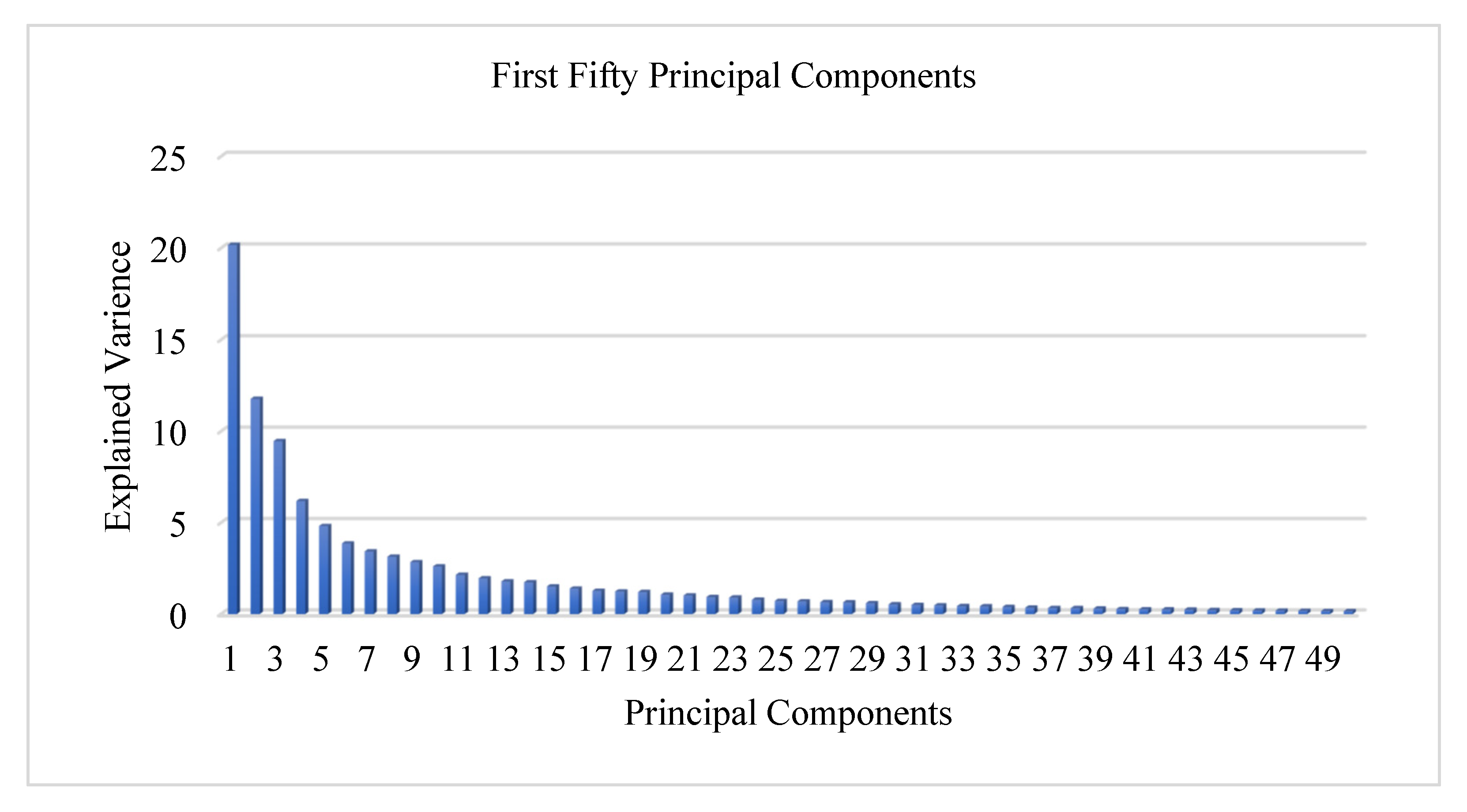
| First PC | 20.17% |
| First two PCs | 31.95% |
| First three PCs | 41.41% |
| First ten PCs | 68.24% |
| First twenty PCs | 83.51% |
| First thirty PCs | 90.93% |
| First forty PCs | 94.70% |
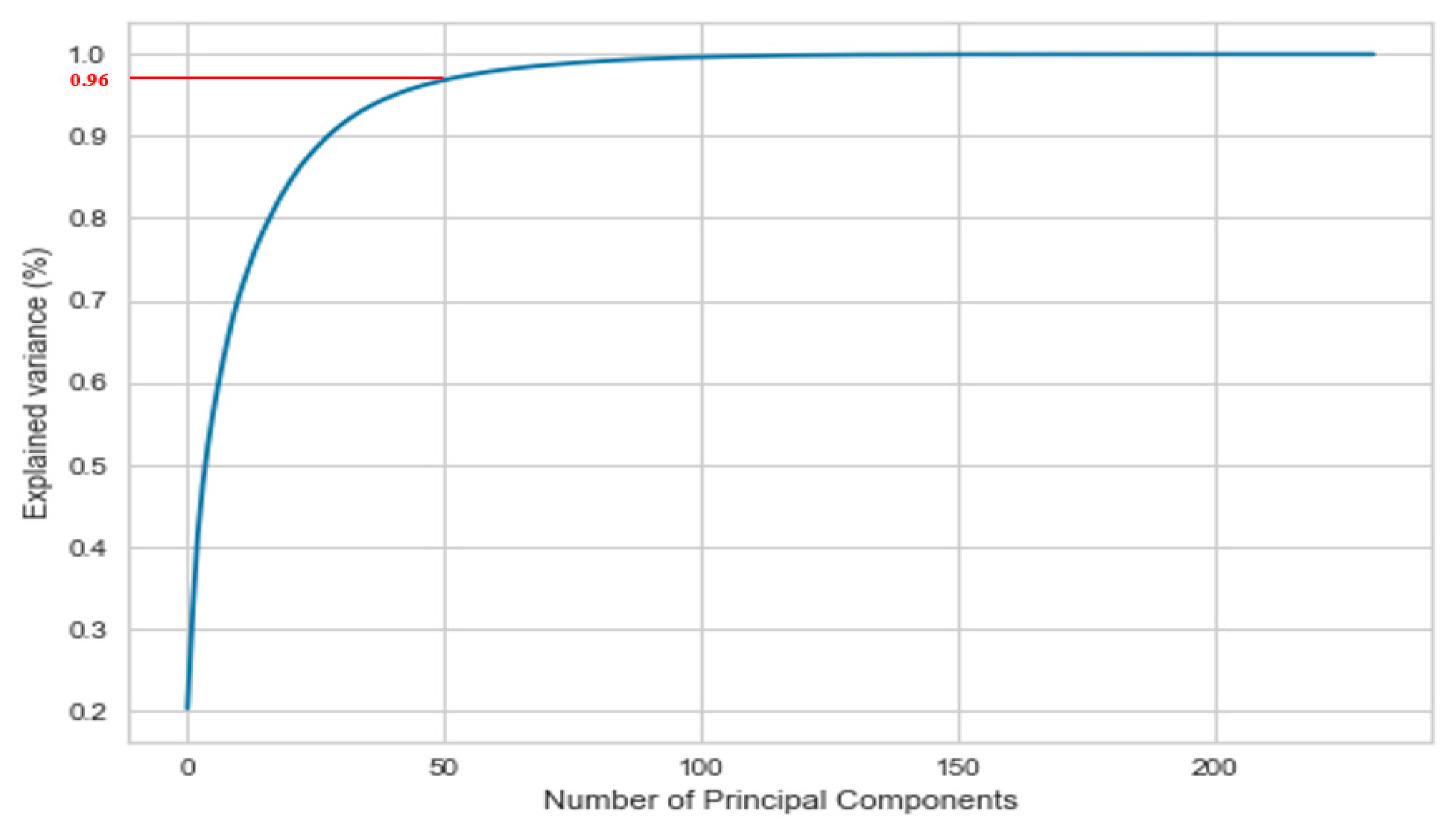
| First fifty PCs | 96.71% |
| C00 | C01 |
| C10 | C11 |
| Hardware Specifications | Software Specifications | ||
|---|---|---|---|
| Processor | Core i5 | OS | 64-bit Windows 10 |
| Processor Clock Speed | 1.8 GHz | Scikit learn | 0.20.3 |
| Number of Cores | 4 | Pandas | 0.23.4 |
| RAM | 8GB | Numpy | 1.14.3 |
| Cache Memory | 6 MB | Matplotlib | 3.0.2 |
| Processor Architecture | 64 bit | Seaborn | 0.11.1 |
| Processor Variant | 8265U | Imblearn | 0.00 |
| SVM Parameters | |||||||
|---|---|---|---|---|---|---|---|
| Parameter | Value | Parameter | Value | Parameter | Value | Parameter | Value |
| C | 2 | kernal | linear | degree | 3 | gamma | auto |
| coef0 | 0.0 | shrinking | True | probability | False | tol | 0.001 |
| cache_ size | 200 | class_ weight | None | verbose | False | max_iter | −1 |
| decision_ function_ shape | ovr | break_ties | False | random_ state | None | ||
| SGD Parameters | |||||||
| Parameter | Value | Parameter | Value | Parameter | Value | Parameter | Value |
| loss | log | penalty | elasticnet | Alpha | 0.0001 | l1_ratio | 0.15 |
| fit_ intercept | true | max_iter | 75 | Tol | 0.001 | shuffle | True |
| verbose | 0 | epsilon | 0.1 | n_jobs | None | random_ state | 0 |
| learning_ rate | optimal | eta0 | 0.0 | power_t | 0.5 | early_ stopping | False |
| validation_ fraction | 0.1 | n_iter_ no_change | 5 | class_ weight | None | warm_start | False |
| KNN Parameters | |||||||
| Parameter | Value | Parameter | Value | Parameter | Value | Parameter | Value |
| n_neighbor | 5 | weight | uniform | algorithm | auto | leaf_ size | 30 |
| p | 2 | metric | minkowski | metric_ param | None | n_jobs | None |
| Elements | TP | FP | FN | TN |
|---|---|---|---|---|
| SVM | 111 | 02 | 01 | 24 |
| KNN | 97 | 08 | 14 | 19 |
| SGD | 101 | 09 | 08 | 20 |
| Measures | SVM | KNN | SGD |
|---|---|---|---|
| Accuracy | 0.9782608 | 0.8405797 | 0.876812 |
| Precision | 0.9823008 | 0.923809 | 0.918182 |
| Recall | 0.9910714 | 0.8738738 | 0.926606 |
| F1-Score | 0.9866666 | 0.8981474 | 0.922375 |
| AUC-ROC | 0.987123 | 0.8366731 | 0.905619 |
| Measures | Min | Max | No. of Max | Mean | SD | |
|---|---|---|---|---|---|---|
| Accuracy | SVM | 0.955882 | 1.00 | 1 | 0.975256 | 0.013813 |
| KNN | 0.855073 | 0.956521 | 0 | 0.908299 | 0.031193 | |
| SGD | 0.594203 | 0.971014 | 0 | 0.83241 | 0.14894 | |
| Precision | SVM | 0.75 | 1.00 | 4 | 0.912387 | 0.092426 |
| KNN | 0.50 | 1.00 | 6 | 0.917188 | 0.155584 | |
| SGD | 0.5 | 0.857143 | 0 | 0.671813 | 0.125704 | |
| Recall | SVM | 0.80 | 1.00 | 4 | 0.921715 | 0.081782 |
| KNN | 0.20 | 0.70 | 0 | 0.434395 | 0.174226 | |
| SGD | 0.496410 | 1.00 | 2 | 0.778064 | 0.194074 | |
| F1-Score | SVM | 0.80 | 1.00 | 2 | 0.913957 | 0.069245 |
| KNN | 0.333333 | 0.823529 | 0 | 0.565863 | 0.173928 | |
| SGD | 0.503737 | 0.923077 | 0 | 0.715369 | 0.146808 | |
| AUC-ROC | SVM | 0.891379 | 1.00 | 1 | 0.949 | 0.038459 |
| KNN | 0.60 | 0.85 | 0 | 0.713385 | 0.086626 | |
| SGD | 0.366071 | 0.984127 | 0 | 0.667223 | 0.267143 | |
Publisher’s Note: MDPI stays neutral with regard to jurisdictional claims in published maps and institutional affiliations. |
© 2021 by the authors. Licensee MDPI, Basel, Switzerland. This article is an open access article distributed under the terms and conditions of the Creative Commons Attribution (CC BY) license (https://creativecommons.org/licenses/by/4.0/).
Share and Cite
Hussain, S.; Raza, Z.; Giacomini, G.; Goswami, N. Support Vector Machine-Based Classification of Vasovagal Syncope Using Head-Up Tilt Test. Biology 2021, 10, 1029. https://doi.org/10.3390/biology10101029
Hussain S, Raza Z, Giacomini G, Goswami N. Support Vector Machine-Based Classification of Vasovagal Syncope Using Head-Up Tilt Test. Biology. 2021; 10(10):1029. https://doi.org/10.3390/biology10101029
Chicago/Turabian StyleHussain, Shahadat, Zahid Raza, Giorgio Giacomini, and Nandu Goswami. 2021. "Support Vector Machine-Based Classification of Vasovagal Syncope Using Head-Up Tilt Test" Biology 10, no. 10: 1029. https://doi.org/10.3390/biology10101029
APA StyleHussain, S., Raza, Z., Giacomini, G., & Goswami, N. (2021). Support Vector Machine-Based Classification of Vasovagal Syncope Using Head-Up Tilt Test. Biology, 10(10), 1029. https://doi.org/10.3390/biology10101029