Highlights
What are the main findings?
- An innovative approach combining acoustic emission (AE) and machine learning (ML) was developed to predict stress levels during mechanical testing of 3D-printed biocomposites.
- AE signal analysis using K-means clustering identified three distinct damage modes: matrix cracking, fiber debonding, and fiber pullout, validated by SEM observations.
What is the implication of the main finding?
- This integrated approach provides a non-destructive monitoring framework for bio-composites, enhancing real-time understanding of damage evolution.
- These findings pave the way for optimizing biocomposite materials by improving fi-ber–matrix bonding to enhance mechanical strength.
Abstract
This paper offers an experimental approach that integrates acoustic emission (AE) monitoring with machine learning (ML) to identify damage mechanisms and predict the mechanical properties of 3D-printed biocomposites. Specimens were fabricated using a bio-filament composed of a PLA matrix reinforced with 10% wt. of Lygeum spartum fibers and were subjected to tensile and flexural tests. The processed dataset, comprising six normalized features (cumulative rise, duration, count, frequency, energy, and amplitude) was used to train four ML models: Random Forest Regression (RFR), Support Vector Regression (SVR), Artificial Neural Networks (ANN), and Decision Trees (DT) implemented in Python using libraries such as scikit-learn, pandas, and numpy. The prediction models were developed using an 80/20 train–test split and further validated by 5-fold cross-validation, with performance evaluated by R-squared (R2) and Mean Squared Error (MSE) metrics. Our results demonstrate robust prediction capabilities, with the RFR model achieving the highest accuracy (R2 > 0.98 and MSE as low as 0.013 for tensile stress prediction). Additionally, unsupervised clustering using K-means was applied to group AE signals into distinct clusters corresponding to different damage modes. This comprehensive methodology not only enhances our understanding of damage evolution in composite materials but also establishes a data-driven framework for non-destructive evaluation and structural health monitoring.
1. Introduction
Advances in 3D printing technology have revolutionized materials science, enabling the rapid prototyping of complex structures with enhanced mechanical and sustainable properties. Among these innovations, biocomposite materials blending natural fibers with biodegradable polymers like polylactic acid (PLA) have emerged as eco-friendly alternatives to conventional synthetic composites. These materials not only reduce environmental impact but also offer competitive strength, stiffness, and lightweight characteristics, making them ideal for automotive, aerospace, and biomedical applications [1,2,3].
A particularly novel aspect of our work is the integration of plant-based Lygeum Spartum fiber into a bio-based PLA polymer for 3D printing to enhance the mechanical performance of printed objects. Numerous studies have examined 3D printing of biocomposites; for example, Le Duigou, A., et al. [4] demonstrated that a 0° printing orientation with reduced thickness yields optimal properties, while Nadir, Ayrilmis, et al. [1] showed that thinner layers improve material performance by influencing porosity and water absorption. Bianchi, Iacopo, et al. [5] compared glass fiber-reinforced polyamide with PLA/hemp composites, highlighting environmental concerns with synthetic reinforcements, and Tao, Yubo, et al. [6] reported that adding wood flour can enhance stress resistance and degradation temperature. Guo, Rui, et al. [7] further illustrated that incorporating toughening agents such as thermoplastic polyurethane improves composite toughness. These studies underscore the potential of natural fibers and optimized printing parameters to enhance composite mechanical properties.
Acoustic emission (AE) analysis has emerged as a crucial tool for real-time monitoring of composite materials by detecting microstructural events such as fiber breakage and matrix cracking [8,9,10]. For instance, Karami et al. [11] employed the Wavelet Packet Transform to identify the factors underlying damage in wood–bioplastic nanocomposites, highlighting AE’s capacity to distinguish between various failure modes. Salje et al. [12] further demonstrated AE’s potential in early failure detection by emphasizing the relationship between AE signals and material degradation. Similarly, Hao et al. [13] utilized wavelet transformation to analyze the time-frequency characteristics of AE signals, effectively classifying damage modes in 3D braided composite shafts. Finally, Ciaburro and Iannace [14] reviewed methodologies for implementing AE techniques in materials and structure condition evaluation, with an emphasis on novel machine learning algorithms for identifying damages, localization, breakage assessment, and failure mode identification. These studies highlight the growing use of AE signal analysis, which could be relevant for studying the characteristics of composite materials. Their applications provide valuable knowledge into the correlation between acoustic signals and the mechanical integrity of composites.
Machine learning (ML) has been increasingly applied for data analysis and predictive modeling in materials science. Several studies have effectively employed ML methods to classify damage mechanisms and estimate mechanical characteristics based on AE features such as cumulative count, energy, and hit to evaluate and quantify damage in composite materials [15,16,17,18,19]. However, predicting the future mechanical properties of composites using AE data remains challenging [20] due to the numerous and overlapping parameters present in AE bursts. Recent advances in ML provide promising solutions for these challenges [9,21,22]. For example, Zhou, W., et al. [23] applied k-means clustering to study damage mechanisms in 3D woven composites, demonstrating that ML can reveal patterns in complex datasets that are difficult to detect using traditional methods. Almeida, Renato SM, et al. [24] introduced an innovative approach to isolate and test individual composite constituents (e.g., matrix, fibers, and interfaces) under tensile loading, enabling precise identification of damage mechanisms such as matrix cracking, fiber breakage, and interfacial debonding through KNN analysis of acoustic emission (AE) signals, achieving 88% classification accuracy. While this method provides critical insights into synthetic composites, its extension to biocomposites and real-time mechanical property prediction remains unexplored. Nonetheless, the quality of training data is critical; researchers like Lu et al. [25] have used ANN models to predict tensile load from AE features, and Sause et al. [26] presented an ANN model for estimating material failure strength, although its predictive capability was limited by the available AE data. To enhance generalizability, larger datasets are required. Random Forest Regression (RFR) has also been widely employed in materials science. Shimamoto et al. [27] used RFR to assess mechanical properties and damage evolution in concrete, while Wang, Zimo, et al. [28] applied it to predict fiber orientation in biocomposites from AE signals. Additionally, Ai et al. [29] tested two techniques, random forest and linear regression, to estimate damage progression, finding that random forest outperformed linear regression.
In this study, a comprehensive framework was developed and validated, integrating biocomposite fabrication, acoustic emission monitoring, and machine learning-based analysis to evaluate and predict the mechanical behavior of a novel biodegradable composite. The key contributions of our work are summarized as follows:
- Development of a biodegradable composite based on a PLA matrix reinforced with plant fiber Lygeum Spartum for 3D printing.
- Evaluation of the mechanical properties of the biocomposite in comparison with neat PLA.
- Application of acoustic emission (AE) monitoring during mechanical testing to capture damage evolution, combined with k-means clustering to classify microstructural damage mechanisms.
- Exploration of various techniques for AE data preparation, including noise reduction, normalization, and feature selection.
- Implementation of four ML models for predicting stress levels, with performance evaluated using metrics such as R2 and MSE.
- Investigation of the most influential AE features to guide future input selection.
This paper is structured as follows: Section 2 describes the experimental methods, including biocomposite production, mechanical testing procedures, and AE data acquisition and cleaning. Section 3 presents the mechanical test results, a comparison between neat PLA and the biocomposite, the evolution and classification of damage using k-means and the ML prediction outcomes. Finally, Section 4 concludes the paper and outlines future directions for research in composite structural health monitoring.
2. Materials and Methods
2.1. Materials and Feed Filament Production
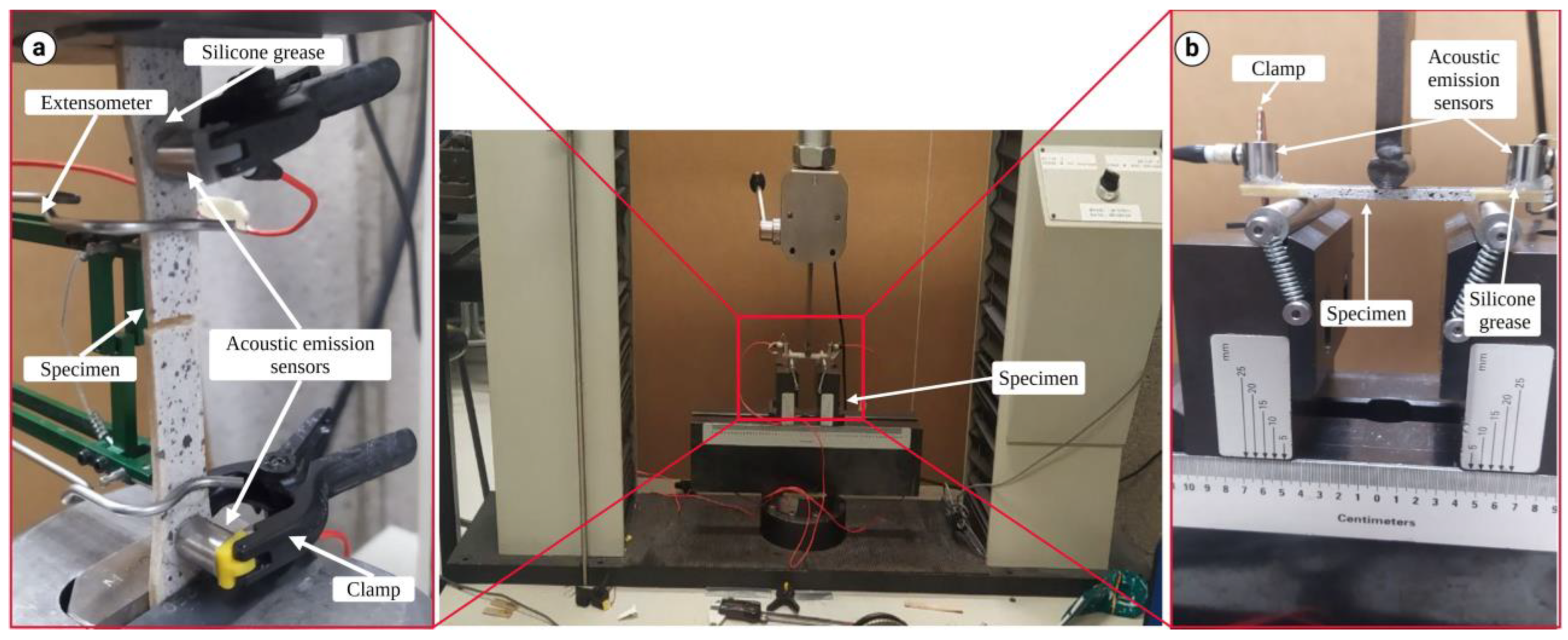
3D printing was used to create biocomposite samples with polylactic acid (PLA) as the matrix material and lignocellulosic (L.S) fibers for reinforcement. Before being introduced into the PLA, the fibers were treated with a 5% sodium hydroxide (NaOH) solution to improve bonding with the polymer matrix. After treatment, the fibers were dried, crushed, and sieved to a small particle size. PLA 4043D Ingeo™ Bio-polymer (NatureWorks LLC, Plymouth, MN, USA; melting point: 150–160 °C, density: 1.24 g/cm3) was combined with treated fibers to produce a composite filament with 10% wt. The resulted composite granules were extruded to produce a 1.75 mm filament diameter for 3D printing. The samples were produced on a 3D printer (CR 10—Creality Technology, Shenzhen, China) equipped with a 0.8 mm nozzle, 900 mm/min print speed, and bed and extrusion temperature of 80 °C and 180 °C, respectively. The mechanical performance of the printed biocomposites (see Figure 1) was assessed using tensile and flexural tests.
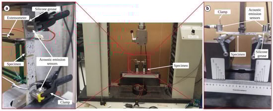
Figure 1.
LS/PLA biocomposite specimens produced through 3D printing and the acoustic emission setup for tensile test (a) and flexural test (b).
2.2. Mechanical Testing and Acoustic Emission Signal Recording
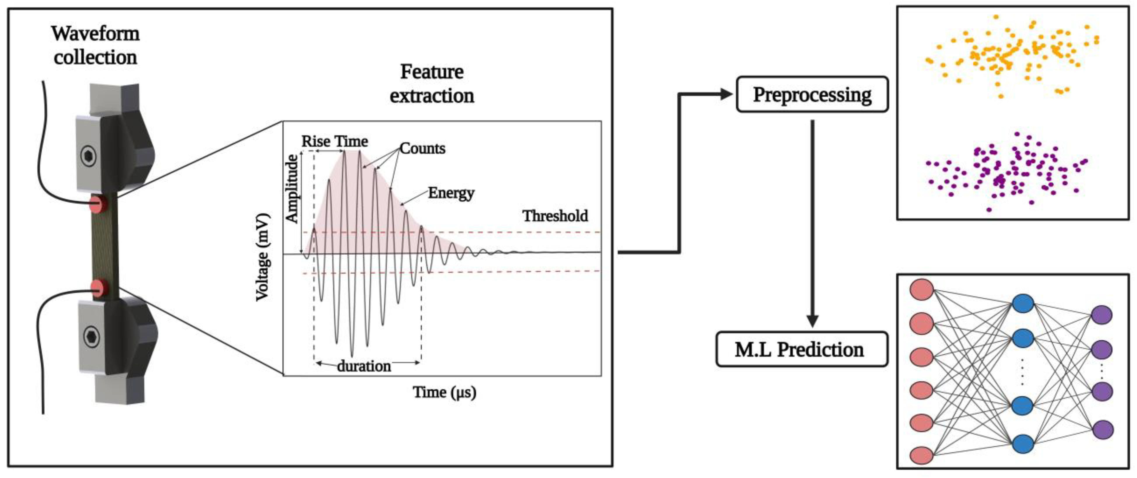
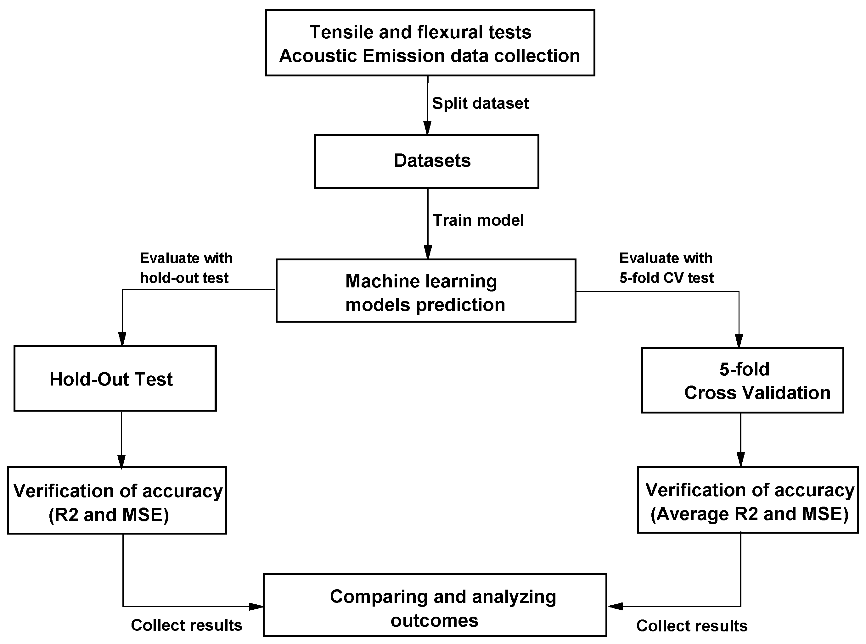
Tensile and flexural tests were performed on these biocomposite samples to evaluate their mechanical properties (Figure 1). An Instron LM-U150 electromechanical testing equipment with a 50 kN load capacity was used for these tests, which were carried out at room temperature. According to ASTM D638 standard [30], specimens with dimensions of 3.2 × 13 × 165 mm (H × W × L) were used for tensile testing. A crosshead speed of 1 mm/min was used, and strain measurements were collected with a 55 mm extensometer. The ASTM D790 [31] standard was followed for performing flexural testing on specimens measuring 3.2 × 13 × 80 mm (H × W × L), a crosshead speed of 2.5 mm/min, and a two-point bending arrangement with a 50 mm support span. Each test was repeated four times. Simultaneously, A two-channel physical data acquisition system (MISTRAS, Princeton Junction, NJ, USA) operating at a 4 MHz sampling rate with 40 dB pre-amplification was used for collecting acoustic emission (AE) data. Two resonant MICRO-80 sensors were used to detect AE signals from 100 to 1000 kHz with a 35 dB threshold to eliminate the noise. The steps for preprocessing acoustic emission data and preparing it for machine learning prediction are shown in Figure 2.

Figure 2.
Experimental procedure for recording acoustic emissions and preparing the data for machine learning prediction.
2.3. Machine Learning Models
In this study, six input features—cumulative rise, duration, count, frequency, energy, and amplitude—from acoustic emission data were utilized to train four machine learning models that predicted stress levels for 3D-printed biocomposite specimens under mechanical testing. These models, including Random Forest Regression (RFR), Support Vector Regression (SVR), Artificial Neural Network (ANN), and Decision Tree (DT) were selected based on their ability to balance performance, interpretability, and computational efficiency. Since we have a limited number of features, normalized data, and a moderate dataset size, RFR, SVR, ANN, and DT provide a robust framework for capturing complex relationships without overcomplicating the training process. Normalization of these features was done to guarantee consistent scaling for all variables. To achieve optimal performance, specific parameters within each model were fine-tuned through hyperparameter optimization (Table 1). Beyond a standard 80/20 train–test split, the training process incorporated rigorous 5-fold cross-validation to assess model generalizability and accuracy. Model performance was evaluated using R-squared and Mean Squared Error (MSE) metrics. These metrics were calculated for each cross-validation fold and the holdout test set (Figure 3).

Table 1.
Hyperparameter tuning and the optimized values for the ML algorithms.
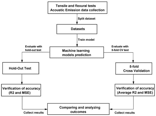
Figure 3.
Machine learning prediction methodology.
To achieve optimal model performance, it is critical to mitigate the risks of overfitting and underfitting. Overfitting occurs when a model fits too much training data, impairing its ability to generalize to unseen data. Techniques such as normalization, early stopping, and hyperparameter tuning [32]. counteract this by simplifying model complexity. Conversely, underfitting arises when a model fails to capture underlying data patterns, performing poorly on both training and test sets. This can be addressed by increasing training time, optimizing hyperparameters, or adopting more sophisticated architectures [33,34].
In this study, normalized data and techniques, such as early stopping and hyperparameter fine-tuning guided by 5-fold cross-validation, struck a balance between these extremes. For example, limiting tree depth in ensemble models and optimizing regularization parameters in support vector regression ensured robustness against noise while retaining predictive power. Similarly, calibrated training epochs and network architectures prevented overtraining in neural networks.
2.4. Preparation of Acoustic Emission Data
The acoustic emission (AE) data was cleaned to eliminate outliers, mostly generated by undesired noise from mechanical friction, electromechanical components, and ambient noise. These disturbances can affect the frequency content and amplitude of the recorded signals. To minimize their impact, a 35 dB amplitude threshold was applied to filter out low-energy noise, ensuring that only meaningful AE events were retained. If not filtered, these disturbances can lead to outliers in the AE data [14,35,36]. The Interquartile Range (IQR) approach was then employed for outlier elimination to improve the accuracy of our predictive and classification models. Extreme values were identified using the IQR technique, making the dataset utilized for machine learning analysis more accurate and representative.
2.5. Cross-Validation and Hold-Out Evaluation
The hold-out method divides the data set into two separate portions, with 80% used for training and the remaining 20% for evaluation. This split offers a simple method to assess how well a model replies to new untested data.
Based on the hold-out method, cross-validation offers a more dependable statistical technique for adjusting hyperparameters. One of the commonly used cross-validation techniques is the 5-fold CV. Using this process, the dataset was divided into five equal portions. In each iteration of the process, the model is trained in four splits, with the remaining parts utilized for validation. During the course of this cycle’s five repetitions, each of the five components acts as the validation set precisely once. This ensures that every data point was utilized exactly once for both training and validation, enabling a full investigation of the model’s performance throughout the whole dataset [37].
2.6. Verification of Accuracy
Metrics like mean squared error (MSE) and coefficient of determination (R2) are frequently used to assess the performance of models. These metrics offer a thorough understanding of the model’s performance when paired with predicted and actual values plots [38]. Whereas MSE measures the average squared difference between predicted and observed values and provides information about the model’s prediction accuracy, R2 indicates the proportion of the dataset’s variance that the model successfully explains. The calculation of R2 and MSE is outlined as follows:
where denotes the actual observed values from the dataset, while represents the estimated values generated by the regression model. Additionally, refers to the mean of the actual data.
where n refers to the total number of observations, represents the actual values, and is the estimated values by the model.
2.7. Damage Mode Identification Using k-Means Clustering Algorithm
The k-means clustering algorithm is a cornerstone in data analysis, praised for its simplicity and efficacy in determining cluster centers that reflect distinct regions within a dataset. It executes through an iterative two-step process: first, each data point is allocated to the closest cluster center, after which every center of the cluster is recalculated as the mean of the data point assigned to it, as noted by [39]. This assignment is reiterated until no data points remain unassigned. Following this, the centroid positions are refined iteratively until the objective function, J, which is defined as follows:
where measures the squared Euclidean distance between each point and its cluster center. This distance indicates how close each n-th data point is to its cluster center. The operation is repeated until the centroids stabilize, thereby segregating the data into distinct classes that minimize intra-cluster distances [40].
In this study, the k-means algorithm (unsupervised machine learning model) was employed to classify acoustic emission (AE) data into predefined categories based on the AE data recorded during mechanical tests. The number of clusters was determined with insights from scanning electron microscopy (SEM) analysis, linking the count of damage modes directly to the microstructural damage observed in SEM images. This method effectively identified distinct damage modes in the biocomposite materials being tested, categorizing the AE data into three main clusters that correspond to variations in AE parameters.
3. Results and Discussion
3.1. Mechanical Properties
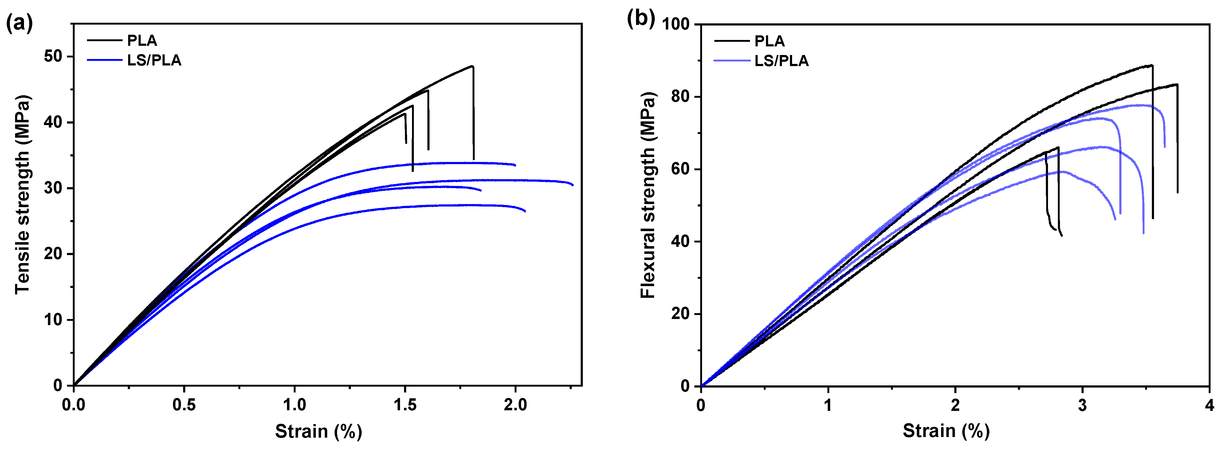
Sixteen specimens of the Lygeum spartum/PLA (LS/PLA) biocomposite and neat PLA were tested for their mechanical properties using tensile and flexural tests. The results are illustrated in a stress–strain curve (Figure 4), representing the relationship between applied stress and material deformation.
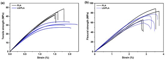
Figure 4.
Typical stress–strain curves for the LS/PLA biocomposite and neat PLA specimens; (a) tensile test, and (b) flexural test.
For tensile testing, LS/PLA specimens exhibited a stress range of 27.45–33.85 MPa, reflecting the biocomposite’s mechanical performance under tensile loading. The strain range was 1.84–2.27%, demonstrating the material’s deformation capacity before failure. The average tensile modulus was 3.24 GPa, indicating stable stiffness and the reinforcing effect of LS fibers. These characteristics highlight the biocomposite’s potential for applications requiring both strength and flexibility.
For flexural testing, LS/PLA specimens displayed a stress range of 64.67–88.76 MPa, with an average value of 75.69 MPa, indicating good flexural strength. The strain range was 2.79–3.74%, with an average value of 3.31%, demonstrating the material’s ability to withstand bending forces.
Regarding neat PLA, the tensile test results showed a higher tensile stress of 44.27 MPa compared to the LS/PLA biocomposite. However, elongation at break was lower (1.61%), indicating reduced ductility. The tensile modulus of 3.4 GPa suggests slightly higher stiffness than the LS/PLA composite. In flexural testing, neat PLA exhibited a flexural stress of 75.69 MPa, with an elongation at break of 3.32% and a flexural modulus of 3.09 GPa. These results indicate that while neat PLA maintains higher tensile strength, the addition of LS fibers improves flexibility and energy absorption, making the biocomposite more suitable for applications requiring a balance of strength, stiffness, and ductility.
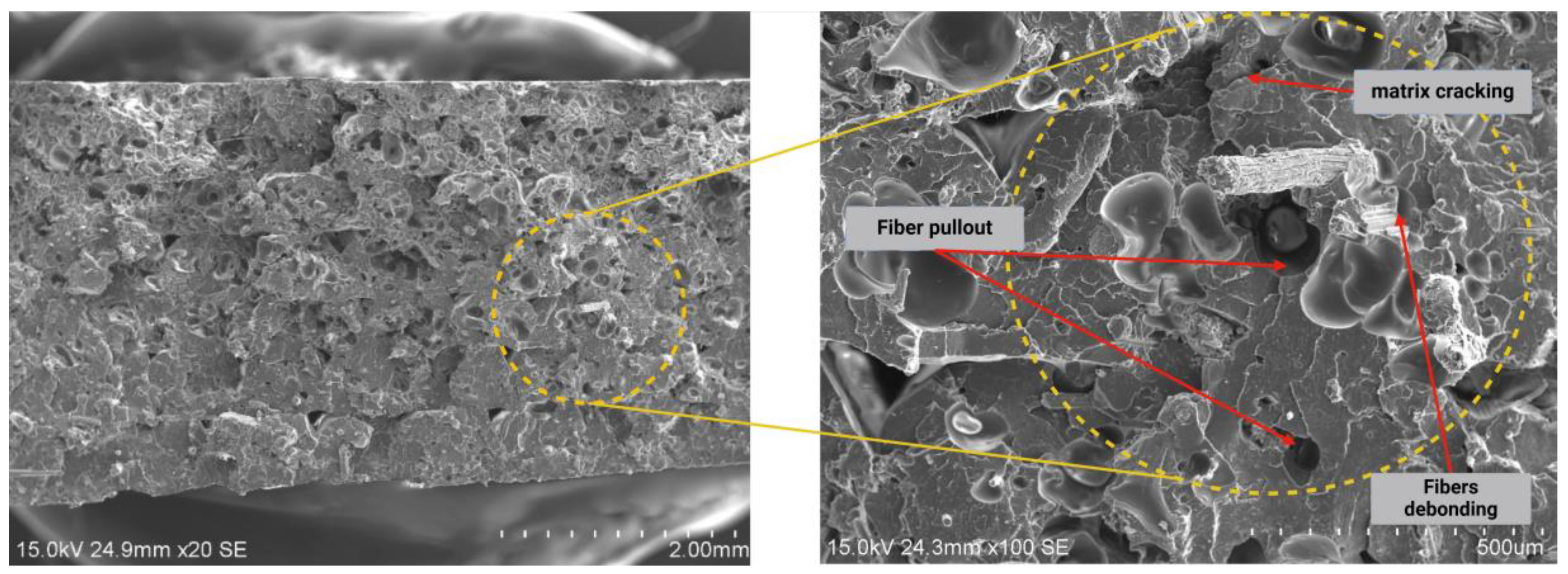
The results indicate the acceptable mechanical properties of the LS/PLA biocomposites, owing to the effective adhesion between the layers and the absence of gaps and voids within the layers. This has been confirmed by SEM images of the cross-sections of the specimens after fracture in Figure 5, showing a coherent and gap-free structure. Such structural integrity in the composite specimens minimizes delamination and enhances material strength, as noted in the literature [41]. The results also showed distinct differences between neat PLA and the LS/PLA biocomposite. Neat PLA exhibited higher tensile strength but lower elongation at break, indicating reduced ductility. In contrast, the LS/PLA composite demonstrated enhanced deformation characteristics, which can be attributed to improved stress transfer between the fiber and the matrix. These findings suggest that further enhancing the bonding at the fiber–matrix interface could optimize the mechanical performance of the biocomposite, improving its energy absorption and overall structural integrity.
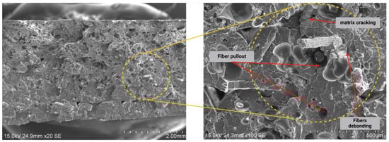
Figure 5.
Fracture surface of the specimen after mechanical testing, highlighting the observed damage mechanisms.
3.2. Analysis of Damage Using Acoustic Emission
3.2.1. Damage Evolution
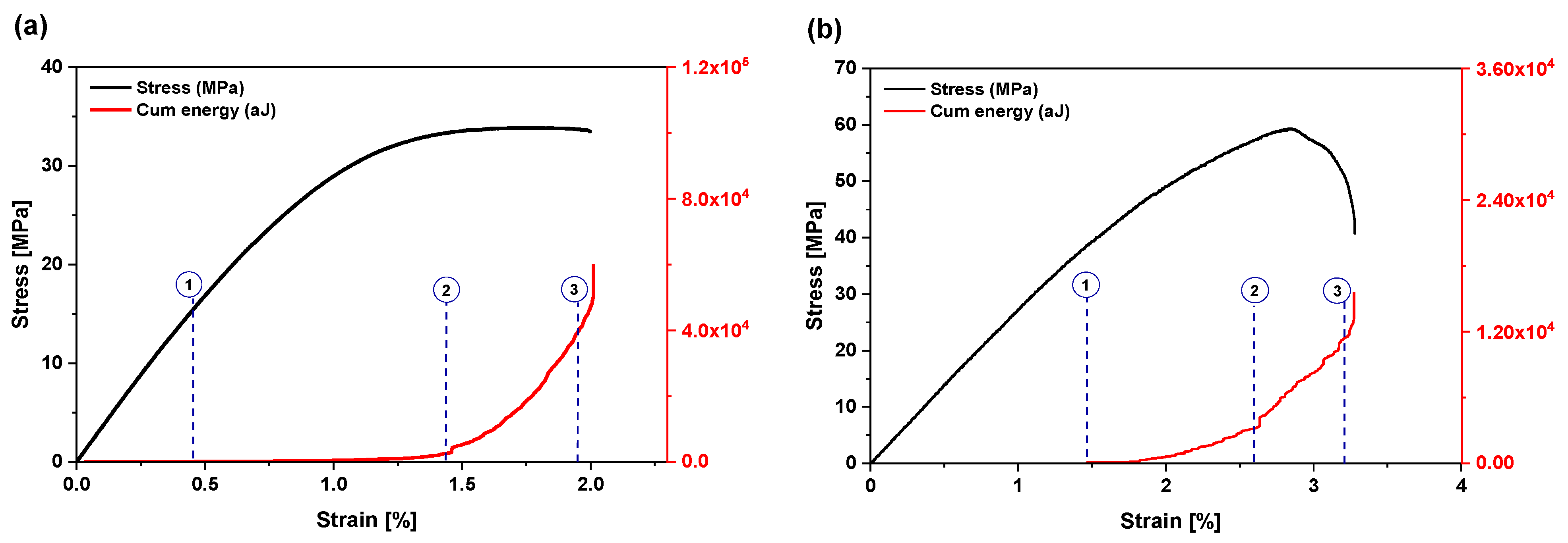
Figure 6 illustrates the curves of stress–strain for LS/PLA composite along with the corresponding AE energy accumulations for both types of tests. For the tensile and flexural tests, the evolution of the acoustic emission (AE) energy shows four distinct phases. The first phase, before position 1 in Figure 6, corresponds to the elastic phase of the deformation curve, where no AE signal is recorded above the noise threshold. The detection of the first significant AE signal marks the beginning of the second phase (zone 1–2). This signal range is related to a specific failure mode in composites, such as matrix cracking. This stage is distinguished by a very low AE activity. At the end of this phase, significant AE activity is observed (point 2). From this point, the AE energy increases exponentially (zone 2–3), indicating an acceleration of damage and the appearance of new failure mechanisms, such as decohesion or fiber–matrix friction. The fourth phase, occurring after point 3, is marked by a sudden increase in energy immediately preceding the final failure.
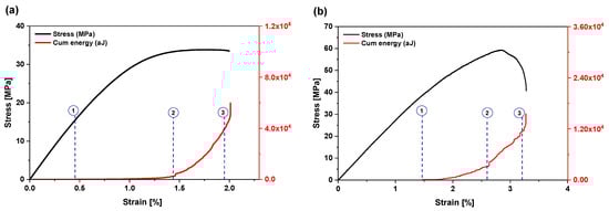
Figure 6.
Stress–strain curves, as well as the cumulative acoustic emission energy, for the composite during tensile (a) and flexural testing (b).
3.2.2. Classification of the Damage Modes Using K-Means Clustering
The changes in mechanical behavior are often linked to variations in failure modes. The accumulated energy of acoustic emission (AE) bursts provides insights into this behavior’s evolution (elastic, plastic phases, etc.). However, more in-depth information can be obtained by applying machine learning-based clustering techniques, such as the K-means algorithm, which leverages the distinct characteristics of AE signals to track the progression of various failure mechanisms during testing.
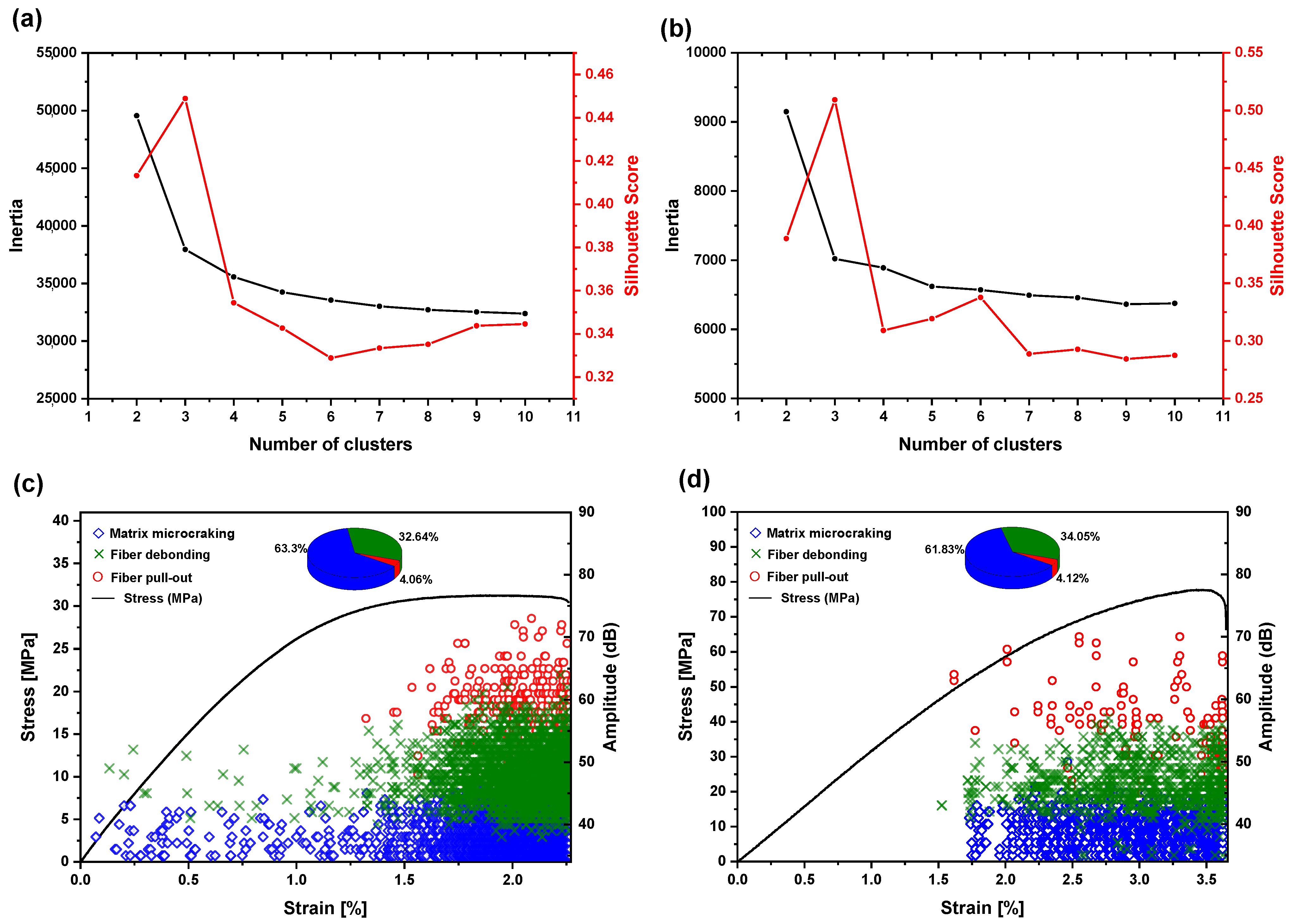
To ensure an optimal selection of clusters, we implemented Silhouette Width Analysis and the Elbow Inertia Method, leading to the identification of three primary clusters. The classification results, presented in Figure 7 for both tensile and flexural tests, align with the existing literature on thermoplastic composites reinforced with natural fibers. The amplitude ranges of AE signals corresponding to specific failure modes were determined as follows: 35–45 dB for matrix cracking, 40–55 dB for fiber debonding, and 50–70 dB for fiber pull-out. These results confirm that failure mechanisms can occur simultaneously, but with varying intensities depending on the material’s response to loading.
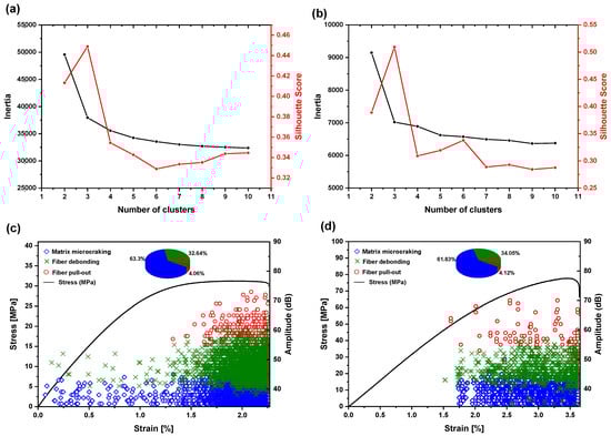
Figure 7.
Silhouette width and elbow inertia for optimal cluster selection: (a) tensile test, (b) flexural test, (c,d) stress–strain curves with AE amplitudes classified by K-means for tensile and flexural tests, respectively.
To validate the clustering-based classification, scanning electron microscopy (SEM) was employed to examine the fracture facies of tested specimens. Figure 5 illustrates the fracture surfaces of tensile-tested specimens, confirming the damage mechanisms identified through AE analysis. The observed fiber–matrix interactions, crack propagation, and fiber pull-out align with the AE-based classification, reinforcing the reliability of the clustering methodology.
3.3. Prediction of Stress Levels in Tensile and Flexural Tests Using Machine Learning Models
3.3.1. Artificial Neural Network ANN
Based on cumulative acoustic emission (AE) features, this work investigates the use of an ANN model to predict the stress levels of 3D-printed biocomposite specimens during tensile and flexural testing. In order to enhance the ANN model, crucial steps were taken, such as choosing relevant AE parameters and eliminating outliers. The model’s structure and the number of layers or nodes was balanced to avoid underfitting and overfitting [42].
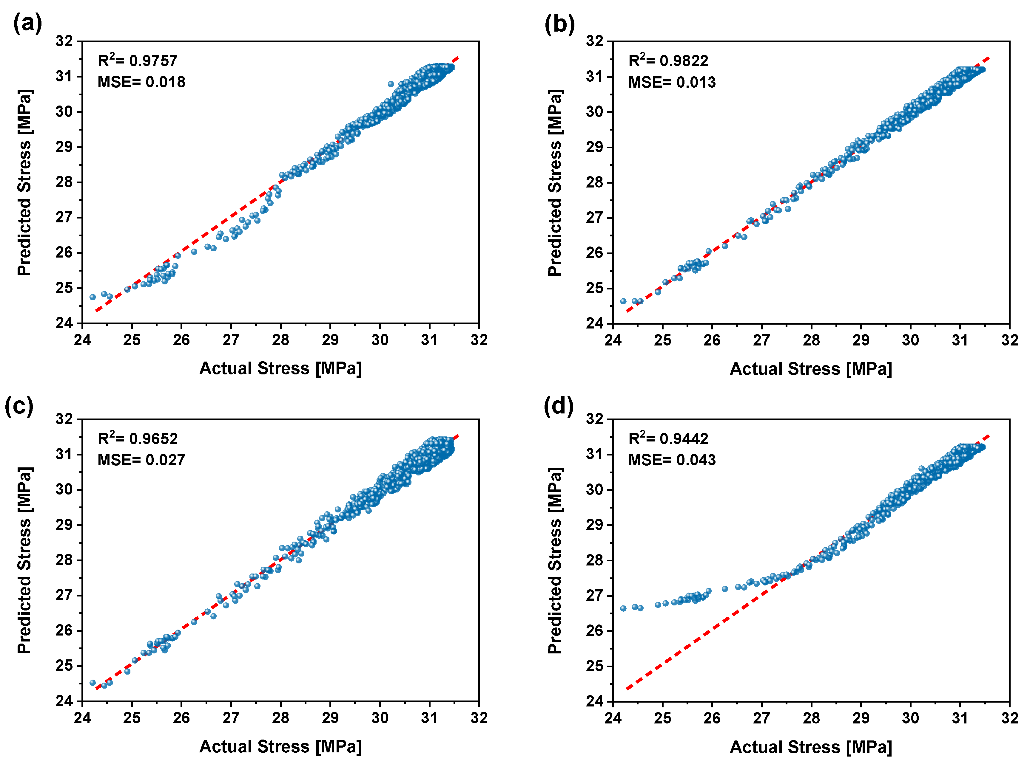
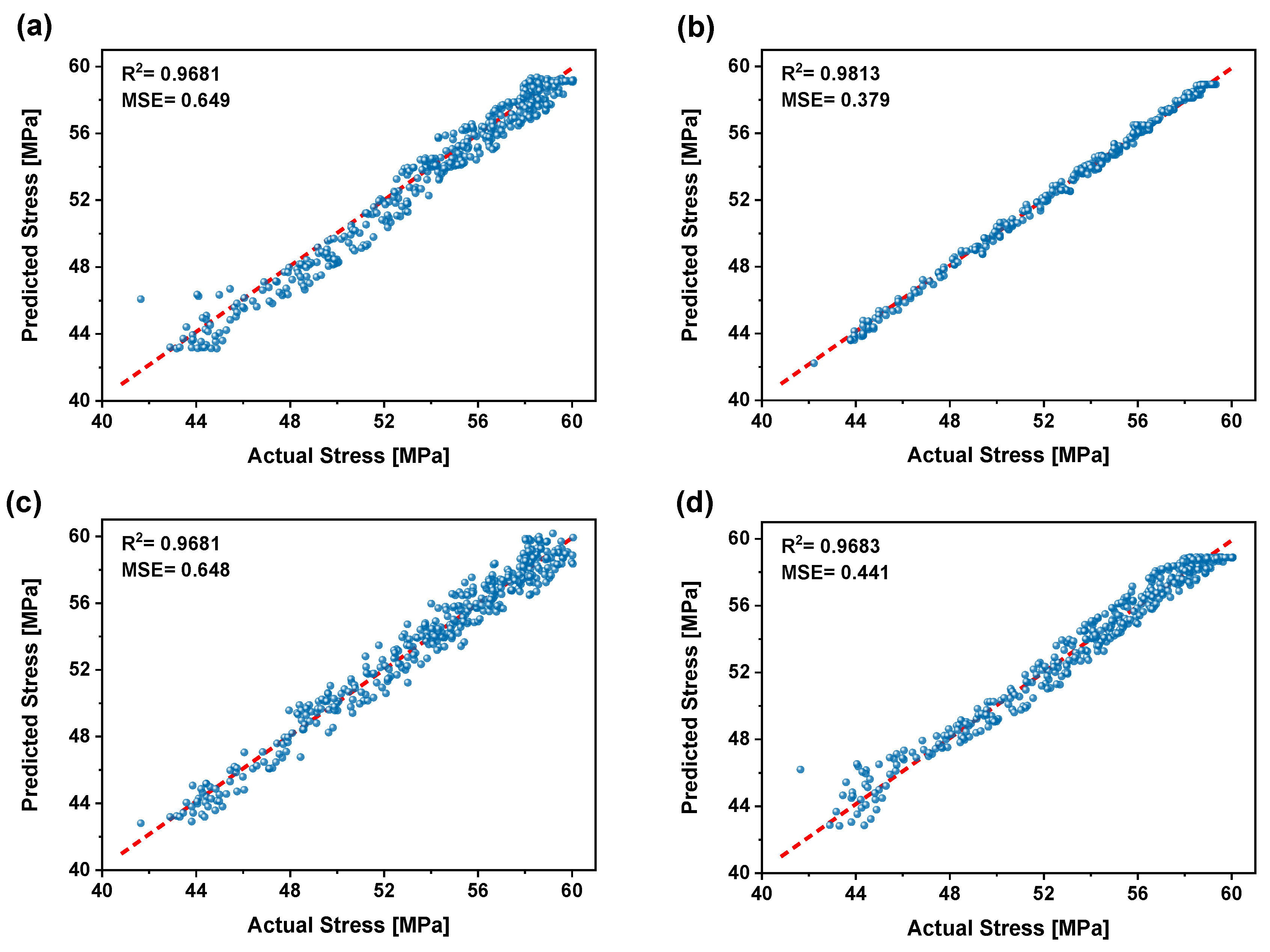
The results, illustrated in Figure 8 and Figure 9, show that the ANN model provides a more accurate prediction for tensile stress (R2 = 0.9757, MSE = 0.0189) compared to the flexural stress (R2 = 0.9681, MSE = 0.6490), indicating a nearly perfect correlation for tensile predictions. This discrepancy in predictive accuracy is attributed to the different mechanical responses of biocomposite under tensile and flexural loads, with tensile tests providing richer AE data due to widespread matrix cracking and other failure mechanisms [43,44].
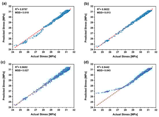
Figure 8.
Stress levels estimated for tensile testing using ML models: (a) ANN, (b) RFR, (c) DTR, and (d) SVR. Blue dots represent the predicted stress values, while the red dashed line indicates perfect prediction—closer proximity to this line reflects better model performance.
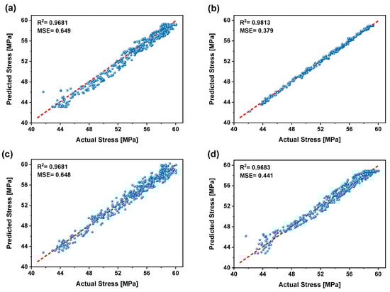
Figure 9.
Stress levels estimated for flexural testing using ML models: (a) ANN, (b) RFR, (c) DTR, and (d) SVR. Blue dots represent the predicted stress values, while the red dashed line indicates perfect prediction—closer proximity to this line reflects better model performance.
Five-fold cross-validation confirmed the model’s reliability, yielding average R2 values of 0.9727 for tensile tests and 0.9575 for flexural tests (Table 2). The study concludes that the diversity and richness of AE data are essential for accurately predicting stress levels, as demonstrated by the superior performance in tensile testing. In contrast, flexural testing predominantly engages the material in the central region where stress is maximized, confining the occurrence of these mechanisms to a localized zone [45]. These result in a more constrained AE signature, potentially limiting the model’s exposure to the full range of signal patterns associated with the material’s failure modes.
Table 2.
A comparison of multiple machine learning models and their performance criteria for both tensile and flexural tests, with acoustic emission parameters inputs.
3.3.2. Random Forest Regression RFR
Feature Importance Analysis
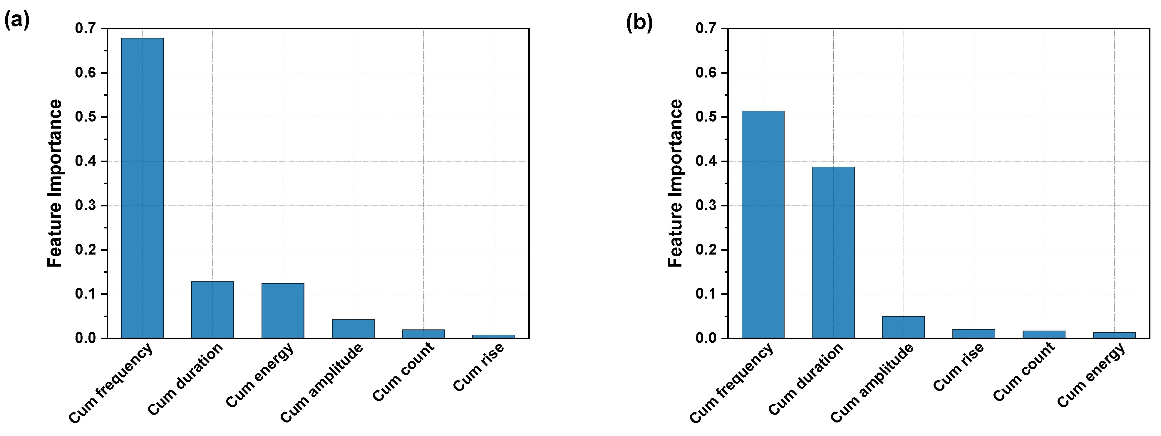
The feature importance analysis within the RFR model highlighted key acoustic emission (AE) signal features correlated with predicted stress levels. Similar to the studies by Shimamoto, Yuma, et al. [27] and Lee, Hang-Lo, et al. [46], the cumulative AE for each feature were used as inputs. The analysis in Figure 10 reveals that cumulative count was the most significant predictor for tensile test, followed by cumulative frequency and duration. Cumulative amplitude, energy, and rise had lesser effects but still contributed nearly equally. For the flexural test, cumulative energy emerged as the most significant predictor, followed by cumulative duration, cumulative count, and cumulative frequency. Cumulative rise and amplitude had the least impact on the model. These findings improve the model and provide thorough knowledge of the relation between mechanical properties and AE signals.
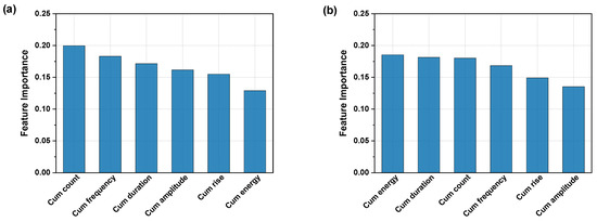
Figure 10.
Feature importance contributing to the predictions of the RFR model for tensile test (a), and flexural test (b).
Stress Level Prediction Using RFR
The scatter plot in Figure 8 and Figure 9 compares predicted to actual stress levels and shows the prediction results for the RFR model. The model demonstrates strong predictive capabilities in predicting the stress levels of this material under both tensile and flexural testing, with an R2 of 0.9822 and MSE of 0.013 for the tensile test. Similarly, the flexural test shows a significant correlation accuracy with an R2 of 0.9813 and an MSE of 0.3792.
The 5-fold cross-validation further validates the results, with an average R2 of 0.9801 for tensile testing and 0.9806 for flexural testing (Table 2), demonstrating the model’s stability and consistency in performance across various data subsets.
3.3.3. Decision Tree Regression DTR
Feature Importance
Feature importance in the DTR model is determined by the extent to which each feature reduces impurity at each split, with greater reductions indicating higher relevance. However, this importance can be less stable than in RFR as it relies on a single tree sensitive to the training data. Figure 11 shows that cumulative frequency is the most important feature compared to the others.
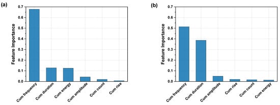
Figure 11.
Feature importance in DT: (a) tensile test and (b) flexural test.
Stress Level Prediction Using DTR
The predicted stress levels estimated by the DT model are illustrated in the scatter plot in Figure 8 and Figure 9. The model demonstrates a high predictive capability, with an R2 score of 0.9652 and an MSE of 0.0271 for the tensile test, and an R2 of 0.9681 and an MSE of 0.6480 for the flexural test. For the 5-fold cross-validation, the model produces consistent results comparable to the holdout test (Table 2). These metrics indicate that the model has solid predictive capabilities for both tests.
By examining the feature importance results from the DT model (Figure 11), the significant differences observed suggest that the model can produce reasonable results by using only the most important features. Specifically, cumulative frequency in the tensile test, and cumulative frequency, cumulative duration, and amplitude in the flexural test, appear as key inputs.
3.3.4. Support Vector Regression SVR
SVR is one of the ML designed for the tasks of regression processes. Unlike typical regression models, the SVR aims to find the hyperplane that optimally fits the data within a preset margin of error. It works by minimizing the error while maximizing the margin, allowing some errors or deviations within a certain threshold (epsilon). The SVR method is especially beneficial for high dimensional data because it may capture complicated connections using kernel functions. These functions convert the used data into a higher dimensional space, and make it easier to find linear relationships that might not be evident in the original space [47].
The estimated stress levels predicted by this model are displayed in Figure 8 and Figure 9. For the tensile test, the model gives an R2 value of 0.9442 and an MSE of 0.0435, while for the flexural test, it attained an R2 of 0.9683 and an MSE of 0.4411.
In the 5-fold cross-validation, the model also achieved R2 values of 0.9526 for tensile testing and 0.9671 for flexural testing, demonstrating stable predictive capabilities across all datasets (Table 2).
3.4. Comparative Performance Analysis of the Employed ML Models
Table 2 presents a comparative analysis of the performance of various machine learning (ML) models. The ANN had challenges with flexural testing, as proven by its MSE and R2 values. Meanwhile, the RFR model, an ensemble technique that leverages the voting mechanism among multiple decision trees, emerged as the most accurate and consistent predictor compared to the rest models. The DT and SVR models, though useful, performed slightly less effectively in both tests, demonstrating limitations in handling the complexity of the dataset.
The RFR model achieved R2 values exceeding 0.98 and MSE as low as 0.013 for tensile stress prediction. The performance differences between tensile and flexural tests are notable; tensile tests provided richer AE data due to the distributed stress along the specimen, whereas flexural tests, where stress is concentrated in the fracture area, resulted in fewer AE events and higher error metrics. These observations indicate that while our models are effective for the current case study, further data collection is needed to ensure generalizability across different loading conditions.
Feature importance analysis used in RFR and DT models revealed that specific AE features play a crucial role in stress prediction. In the RFR model, cumulative energy and count emerged as the most critical predictors, while the DT model indicated that frequency is the dominant feature.
The higher MSE and RMSE values observed in all ML models for the flexural test can be attributed to the smaller dataset relative to the tensile test. Furthermore, the maximum stress in the flexural test exceeds 60 MPa, whereas the tensile test stress remains below 32 MPa. This disparity likely contributes to the consistently elevated MSE and RMSE values in predicting flexural stress as compared to tensile stress.
Despite minor differences in performance, all models exhibited strong predictive capabilities, with the lowest R2 value exceeding 0.94, reflecting high accuracy. This impressive outcome can be attributed to the stability and richness of the data, along with meticulous data preparation. Key factors such as effective outlier removal, coupled with techniques to mitigate overfitting and underfitting including hyperparameter tuning, data normalization, and early stopping significantly enhanced the models’ ability to capture complex relationships within the dataset. Additionally, the thorough approach to data preparation and model training ensured that each model was well-equipped to address the intricacies of both tensile and flexural testing, providing reliable insights into material behavior.
4. Conclusions
This study successfully developed a biocomposite using a PLA matrix reinforced with Lygeum spartum fibers. The biocomposite demonstrated enhanced mechanical properties, including improved elongation at break and elasticity modulus compared to neat PLA. Analysis of cumulative acoustic emission (AE) energy revealed three distinct stages of damage evolution during mechanical testing, while k-means clustering identified three primary damage modes, matrix cracking, fiber debonding, and fiber pull-out which were validated through SEM observations.
Four machine learning models, Random Forest Regression (RFR), Artificial Neural Network (ANN), Decision Tree (DTR), and Support Vector Regression (SVR) were applied to predict stress levels using AE data. Among these, the RFR model outperformed the others, achieving the highest result accuracy by emphasizing critical AE features such as cumulative energy and count. Notably, tensile tests yielded superior predictions compared to flexural tests due to richer AE data from a uniform stress distribution, in contrast to the localized stress concentrations observed during flexural loading.
In conclusion, the integration of acoustic emission data with multiple machine learning models has proven to be an effective approach for health monitoring of biocomposite materials, advancing our ability to predict stress levels and understand damage evolution. This research demonstrates the potential of these techniques to enhance prediction accuracy and provide valuable insights into biocomposite behavior under stress. However, our study also highlights certain limitations; for example, improving stress resistance may require exploring alternative techniques to enhance fiber–matrix bonding, and expanding the dataset to include a larger number of specimens will be essential for developing more generalized and robust predictive models.
Author Contributions
Conceptualization, M.G., Z.B., L.T. and S.E.T.; methodology, K.B., M.G., Z.B. and S.E.T.; formal analysis, K.B., Z.B. and L.T.; investigation, K.B.; resources, Z.B. and L.T.; data curation, K.B. and S.E.T.; writing—original draft preparation, K.B.; writing—review and editing, M.G., Z.B., L.T. and S.E.T.; visualization, K.B.; supervision, M.G. and Z.B.; project administration, Z.B. and L.T. All authors have read and agreed to the published version of the manuscript.
Funding
This research received no external funding.
Data Availability Statement
Data will be made available on request.
Conflicts of Interest
The authors declare no conflicts of interest.
References
- Ayrilmis, N.; Kariz, M.; Kwon, J.H.; Kuzman, M.K. Effect of printing layer thickness on water absorption and mechanical properties of 3D-printed wood/PLA composite materials. Int. J. Adv. Manuf. Technol. 2019, 102, 2195–2200. [Google Scholar] [CrossRef]
- Bahrami, M.; Abenojar, J.; Martínez, M.Á. Recent progress in hybrid biocomposites: Mechanical properties, water absorption, and flame retardancy. Materials 2020, 13, 5145. [Google Scholar] [CrossRef]
- Trivedi, A.K.; Gupta, M.; Singh, H. PLA based biocomposites for sustainable products: A review. Adv. Ind. Eng. Polym. Res. 2023, 6, 382–395. [Google Scholar] [CrossRef]
- Le Duigou, A.; Castro, M.; Bevan, R.; Martin, N. 3D printing of wood fibre biocomposites: From mechanical to actuation functionality. Mater. Des. 2016, 96, 106–114. [Google Scholar] [CrossRef]
- Bianchi, I.; Forcellese, A.; Gentili, S.; Greco, L.; Simoncini, M. Comparison between the mechanical properties and environmental impacts of 3D printed synthetic and bio-based composites. Procedia CIRP 2022, 105, 380–385. [Google Scholar] [CrossRef]
- Tao, Y.; Wang, H.; Li, Z.; Li, P.; Shi, S.Q. Development and application of wood flour-filled polylactic acid composite filament for 3D printing. Materials 2017, 10, 339. [Google Scholar] [CrossRef]
- Guo, R.; Ren, Z.; Bi, H.; Song, Y.; Xu, M. Effect of toughening agents on the properties of poplar wood flour/poly (lactic acid) composites fabricated with Fused Deposition Modeling. Eur. Polym. J. 2018, 107, 34–45. [Google Scholar] [CrossRef]
- Panasiuk, K.; Dudzik, K. Determining the stages of deformation and destruction of composite materials in a static tensile test by acoustic emission. Materials 2022, 15, 313. [Google Scholar] [CrossRef]
- Barile, C.; Casavola, C.; Pappalettera, G.; Kannan, V.P. Damage monitoring of carbon fibre reinforced polymer composites using acoustic emission technique and deep learning. Compos. Struct. 2022, 292, 115629. [Google Scholar] [CrossRef]
- Huijer, A.; Kassapoglou, C.; Pahlavan, L. Acoustic emission monitoring of carbon fibre reinforced composites with embedded sensors for in-situ damage identification. Sensors 2021, 21, 6926. [Google Scholar] [CrossRef]
- Karami, S.; Khamedi, R.; Azizi, H.; Najafabadi, M.A. Investigation of the effect of nanoparticles on wood-bioplastic composite behavior using the acoustic emission method. J. Compos. Mater. 2022, 57, 23–34. [Google Scholar] [CrossRef]
- Salje, E.K.H.; Jiang, X.; Eckstein, J.; Wang, L. Acoustic emission spectroscopy: Applications in geomaterials and related materials. Appl. Sci. 2021, 11, 8801. [Google Scholar] [CrossRef]
- Hao, W.; Huang, Z.; Xu, Y.; Zhao, G.; Chen, H.; Fang, D. Acoustic emission characterization of tensile damage in 3D braiding composite shafts. Polym. Test. 2020, 81, 106176. [Google Scholar] [CrossRef]
- Ciaburro, G.; Iannace, G. Machine-learning-based methods for acoustic emission testing: A review. Appl. Sci. 2022, 12, 10476. [Google Scholar] [CrossRef]
- Habibi, M.; Laperrière, L.; Lebrun, G.; Toubal, L. Combining short flax fiber mats and unidirectional flax yarns for composite applications: Effect of short flax fibers on biaxial mechanical properties and damage behaviour. Compos. Part B Eng. 2017, 123, 165–178. [Google Scholar] [CrossRef]
- Saidane, E.H.; Scida, D.; Assarar, M.; Ayad, R. Damage mechanisms assessment of hybrid flax-glass fibre composites using acoustic emission. Compos. Struct. 2017, 174, 1–11. [Google Scholar] [CrossRef]
- Sobhani, A.; Saeedifar, M.; Najafabadi, M.A.; Fotouhi, M.; Zarouchas, D. The study of buckling and post-buckling behavior of laminated composites consisting multiple delaminations using acoustic emission. Thin-Walled Struct. 2018, 127, 145–156. [Google Scholar] [CrossRef]
- Malpot, A.; Touchard, F.; Bergamo, S. An investigation of the influence of moisture on fatigue damage mechanisms in a woven glass-fibre-reinforced PA66 composite using acoustic emission and infrared thermography. Compos. Part B Eng. 2017, 130, 11–20. [Google Scholar] [CrossRef]
- Roundi, W.; El Mahi, A.; El Gharad, A.; Rebiere, J.-L. Acoustic emission monitoring of damage progression in Glass/Epoxy composites during static and fatigue tensile tests. Appl. Acoust. 2018, 132, 124–134. [Google Scholar] [CrossRef]
- Saeedifar, M.; Zarouchas, D. Damage characterization of laminated composites using acoustic emission: A review. Compos. Part B Eng. 2020, 195, 108039. [Google Scholar] [CrossRef]
- Xu, D.; Liu, P.; Chen, Z. A deep learning method for damage prognostics of fiber-reinforced composite laminates using acoustic emission. Eng. Fract. Mech. 2022, 259, 108139. [Google Scholar] [CrossRef]
- König, F.; Sous, C.; Chaib, A.O.; Jacobs, G. Machine learning based anomaly detection and classification of acoustic emission events for wear monitoring in sliding bearing systems. Tribol. Int. 2021, 155, 106811. [Google Scholar] [CrossRef]
- Zhou, W.; Zhang, Y.; Zhao, W. Tensile Deformation Damage and Clustering Analysis of Acoustic Emission Signals in Three-Dimensional Woven Composites. In Advances in Acoustic Emission Technology: Proceedings of the World Conference on Acoustic Emission-2017; Springer: Berlin/Heidelberg, Germany, 2019. [Google Scholar]
- Almeida, R.S.; Magalhães, M.D.; Karim, N.; Tushtev, K.; Rezwan, K. Identifying damage mechanisms of composites by acoustic emission and supervised machine learning. Mater. Des. 2023, 227, 111745. [Google Scholar] [CrossRef]
- Lu, D.; Yu, W. Predicting the tensile strength of single wool fibers using artificial neural network and multiple linear regression models based on acoustic emission. Text. Res. J. 2020, 91, 533–542. [Google Scholar] [CrossRef]
- Sause, M.G.; Schmitt, S.; Kalafat, S. Failure load prediction for fiber-reinforced composites based on acoustic emission. Compos. Sci. Technol. 2018, 164, 24–33. [Google Scholar] [CrossRef]
- Shimamoto, Y.; Suzuki, T.; Tayfur, S.; Alver, N. Estimation of Concrete Mechanical Properties by Acoustic Emission with Random Forest Algorithm. International Symposium on Non-Destructive Testing in Civil Engineering (NDT-CE 2022), 16–18 August 2022, Zurich, Switzerland. e-J. Nondestruct. Testing 2022, 27. [Google Scholar] [CrossRef]
- Wang, Z.; Chegdani, F.; Yalamarti, N.; Takabi, B.; Tai, B.; El Mansori, M.; Bukkapatnam, S.T. Acoustic emission characterization of natural fiber reinforced plastic composite machining using a random forest machine learning model. J. Manuf. Sci. Eng. 2020, 142, 031003. [Google Scholar] [CrossRef]
- Ai, L.; Flowers, S.; Mesaric, T.; Henderson, B.; Houck, S.; Ziehl, P. Acoustic Emission-Based Detection of Impacts on Thermoplastic Aircraft Control Surfaces: A Preliminary Study. Appl. Sci. 2023, 13, 6573. [Google Scholar] [CrossRef]
- ASTM D638; Standard Test Method for Tensile Properties of Plastics. American Society for Testing and Materials: West Conshohocken, PA, USA, 1998.
- ASTM D790; Standard Test Methods for Flexural Properties of Unreinforced and Reinforced Plastics and Electrical Insulating Materials. Annual Book of ASTM Standards: West Conshohocken, PA, USA, 1997.
- Ying, X. An overview of overfitting and its solutions. J. Phys. Conf. Ser. 2019, 1168, 022022. [Google Scholar] [CrossRef]
- Bashir, D.; Montañez, G.D.; Sehra, S.; Segura, P.S.; Lauw, J. An information-theoretic perspective on overfitting and underfitting. In Proceedings of the AI 2020: Advances in Artificial Intelligence: 33rd Australasian Joint Conference, AI 2020, Proceedings 33, Canberra, ACT, Australia, 29–30 November 2020; Springer: Berlin/Heidelberg, Germany, 2020. [Google Scholar]
- Pothuganti, S. Review on over-fitting and under-fitting problems in Machine Learning and solutions. Int. J. Adv. Res. Electr. Electron. Instrum. Eng. 2018, 7, 3692–3695. [Google Scholar]
- Barsoum, F.F.; Suleman, J.; Korcak, A.; Hill, E.V. Acoustic emission monitoring and fatigue life prediction in axially loaded notched steel specimens. J. Acoust. Emiss. 2009, 27, 40–63. [Google Scholar]
- Benabderazag, K.; Belouadah, Z.; Guebailia, M.; Toubal, L. Characterization of thermomechanical properties and damage mechanisms using acoustic emission of Lygeum spartum PLA 3D-printed biocomposite with fused deposition modelling. Compos. Part A Appl. Sci. Manuf. 2024, 186, 108426. [Google Scholar] [CrossRef]
- Xiong, Z.; Cui, Y.; Liu, Z.; Zhao, Y.; Hu, M.; Hu, J. Evaluating explorative prediction power of machine learning algorithms for materials discovery using k-fold forward cross-validation. Comput. Mater. Sci. 2020, 171, 109203. [Google Scholar]
- Beyeler, M. Machine Learning for OpenCV; Packt Publishing Ltd.: Birmingham, UK, 2017. [Google Scholar]
- Müller, A.C.; Guido, S. Introduction to Machine Learning with Python: A Guide for Data Scientists; O’Reilly Media, Inc.: Newton, MA, USA, 2016. [Google Scholar]
- Hadi, A.S.; Kaufman, L.; Rousseeuw, P.J. Finding Groups in Data: An Introduction to Cluster Analysis; John Wiley & Sons: Hoboken, NJ, USA, 2009. [Google Scholar]
- Djabali, A.; Toubal, L.; Zitoune, R.; Rechak, S. Fatigue damage evolution in thick composite laminates: Combination of X-ray tomography, acoustic emission and digital image correlation. Compos. Sci. Technol. 2019, 183, 107815. [Google Scholar] [CrossRef]
- Karsoliya, S. Approximating number of hidden layer neurons in multiple hidden layer BPNN architecture. Int. J. Eng. Trends Technol. 2012, 3, 714–717. [Google Scholar]
- Li, P.; Zhang, W.; Ye, Z.; Wang, Y.; Yang, S.; Wang, L. Analysis of acoustic emission energy from reinforced concrete sewage pipeline under full-scale loading test. Appl. Sci. 2022, 12, 8624. [Google Scholar] [CrossRef]
- Karthik, M.K.; Kumar, C.S. A comprehensive review on damage characterization in polymer composite laminates using acoustic emission monitoring. Russ. J. Nondestruct. Test. 2022, 58, 705–721. [Google Scholar] [CrossRef]
- Han, S.N.M.F.; Taha, M.M.; Mansor, M.R.; Rahman, M.A.A. Investigation of tensile and flexural properties of kenaf fiber-reinforced acrylonitrile butadiene styrene composites fabricated by fused deposition modeling. J. Eng. Appl. Sci. 2022, 69, 52. [Google Scholar] [CrossRef]
- Lee, H.-L.; Kim, J.-S.; Hong, C.-H.; Cho, D.-K. Ensemble learning approach for the prediction of quantitative rock damage using various acoustic emission parameters. Appl. Sci. 2021, 11, 4008. [Google Scholar] [CrossRef]
- Koya, B.P.; Aneja, S.; Gupta, R.; Valeo, C. Comparative analysis of different machine learning algorithms to predict mechanical properties of concrete. Mech. Adv. Mater. Struct. 2022, 29, 4032–4043. [Google Scholar] [CrossRef]

Disclaimer/Publisher’s Note: The statements, opinions and data contained in all publications are solely those of the individual author(s) and contributor(s) and not of MDPI and/or the editor(s). MDPI and/or the editor(s) disclaim responsibility for any injury to people or property resulting from any ideas, methods, instructions or products referred to in the content. |
© 2025 by the authors. Licensee MDPI, Basel, Switzerland. This article is an open access article distributed under the terms and conditions of the Creative Commons Attribution (CC BY) license (https://creativecommons.org/licenses/by/4.0/).