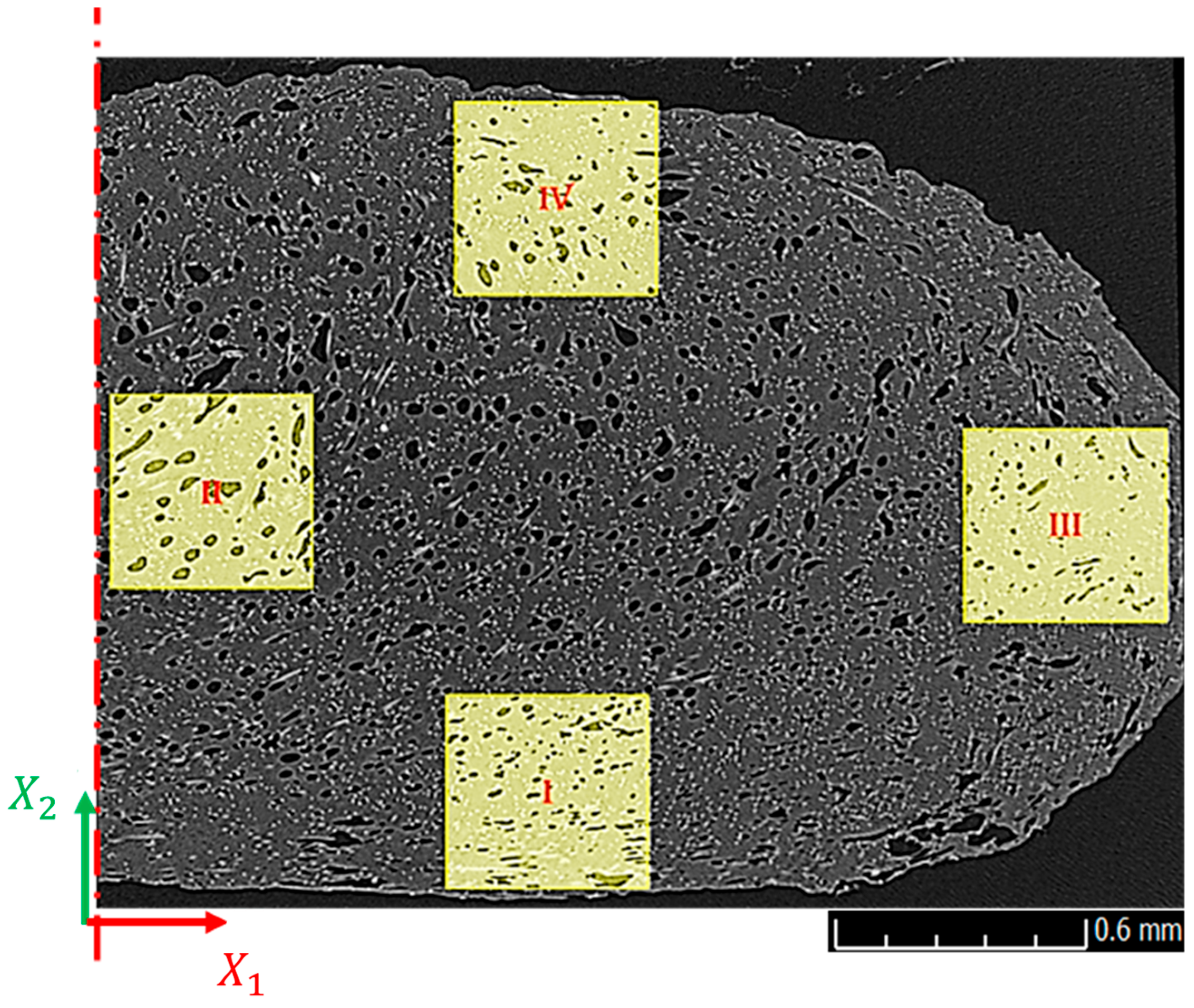
Figure 1.
Regions of interest (ROI, I–IV) of the CF/ABS specimen from a polymer composite bead manufactured using Baylor’s LAAM system. ( and are coordinate directions normal to the print direction , and the red dot dashed line indicates a plane of half-symmetry plane in the direction).
Figure 1.
Regions of interest (ROI, I–IV) of the CF/ABS specimen from a polymer composite bead manufactured using Baylor’s LAAM system. ( and are coordinate directions normal to the print direction , and the red dot dashed line indicates a plane of half-symmetry plane in the direction).
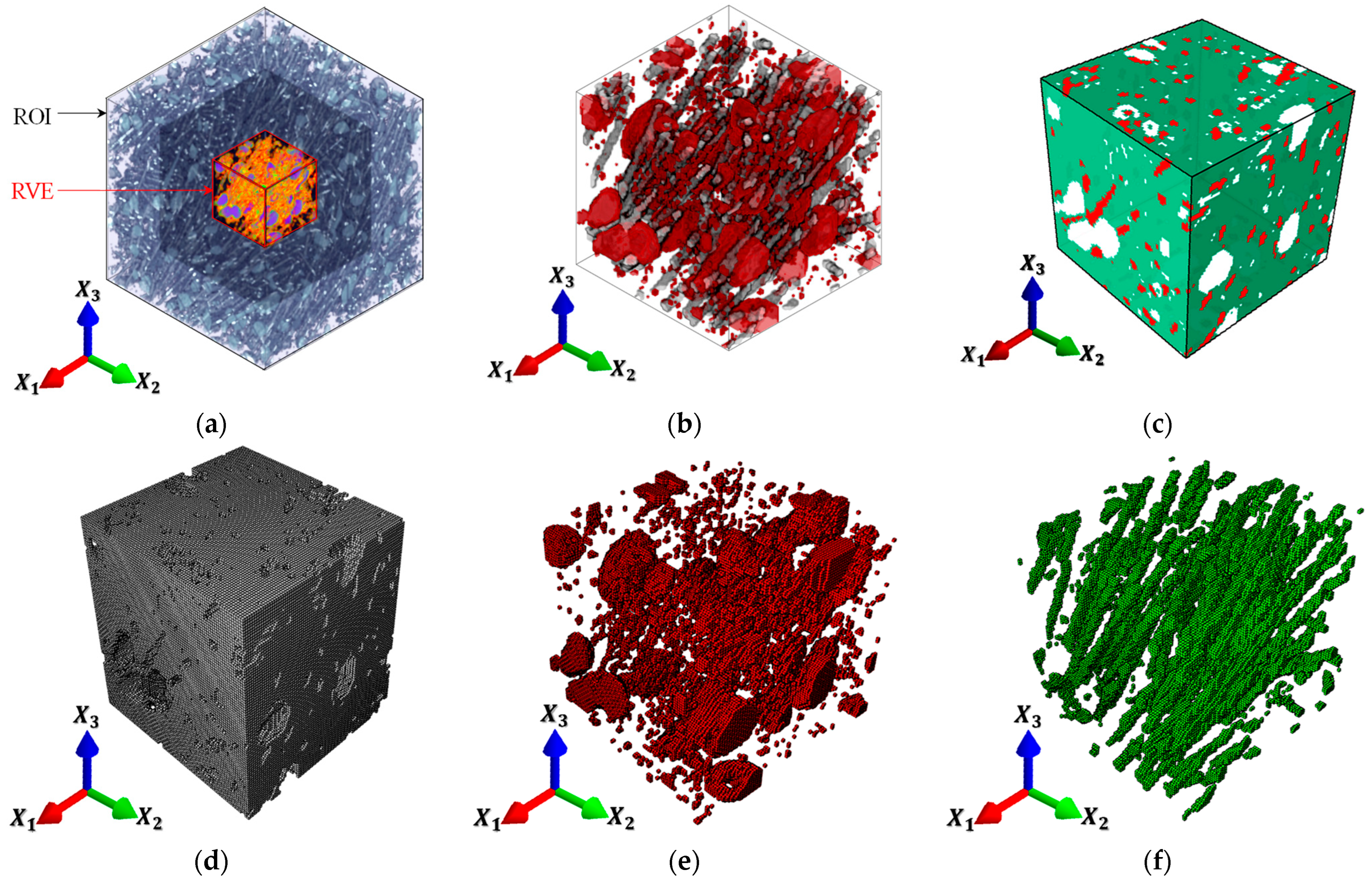
Figure 2.
(a) Reconstructed 3D scans of ROI-II highlighting mid-block RVE volume; (b) magnified view of mid-block RVE showing segmented micro-constituents; (c) FEA model imported from voxel data of the RVE; (d) ABS matrix FEA elements; (e) micro-void FEA elements; and (f) fiber reinforcement FEA elements.
Figure 3.
ROI-II partitioning into (a) RVE—I: 125 realizations with 125,000 elements per realization with ; (b) RVE—II: 27 realizations with 571,787 elements per realization with ; (c) RVE—III: 8 realizations with 1,953,125 elements per realization with .
Figure 3.
ROI-II partitioning into (a) RVE—I: 125 realizations with 125,000 elements per realization with ; (b) RVE—II: 27 realizations with 571,787 elements per realization with ; (c) RVE—III: 8 realizations with 1,953,125 elements per realization with .
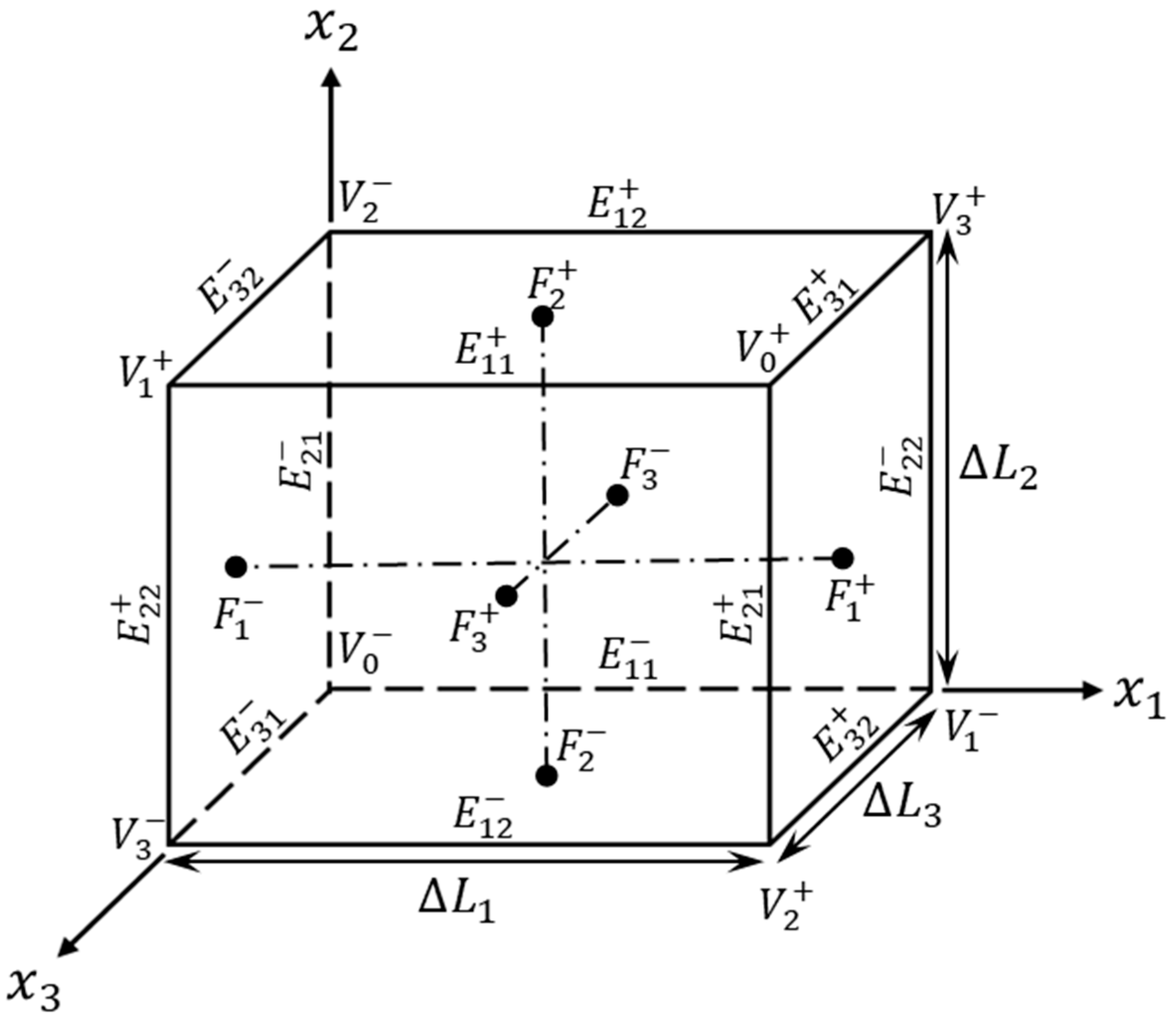
Figure 4.
Single periodic RVE structure showing definitions of entities and coordinate directions used in the PBC formulations (Equations (1)–(3)).
Figure 4.
Single periodic RVE structure showing definitions of entities and coordinate directions used in the PBC formulations (Equations (1)–(3)).
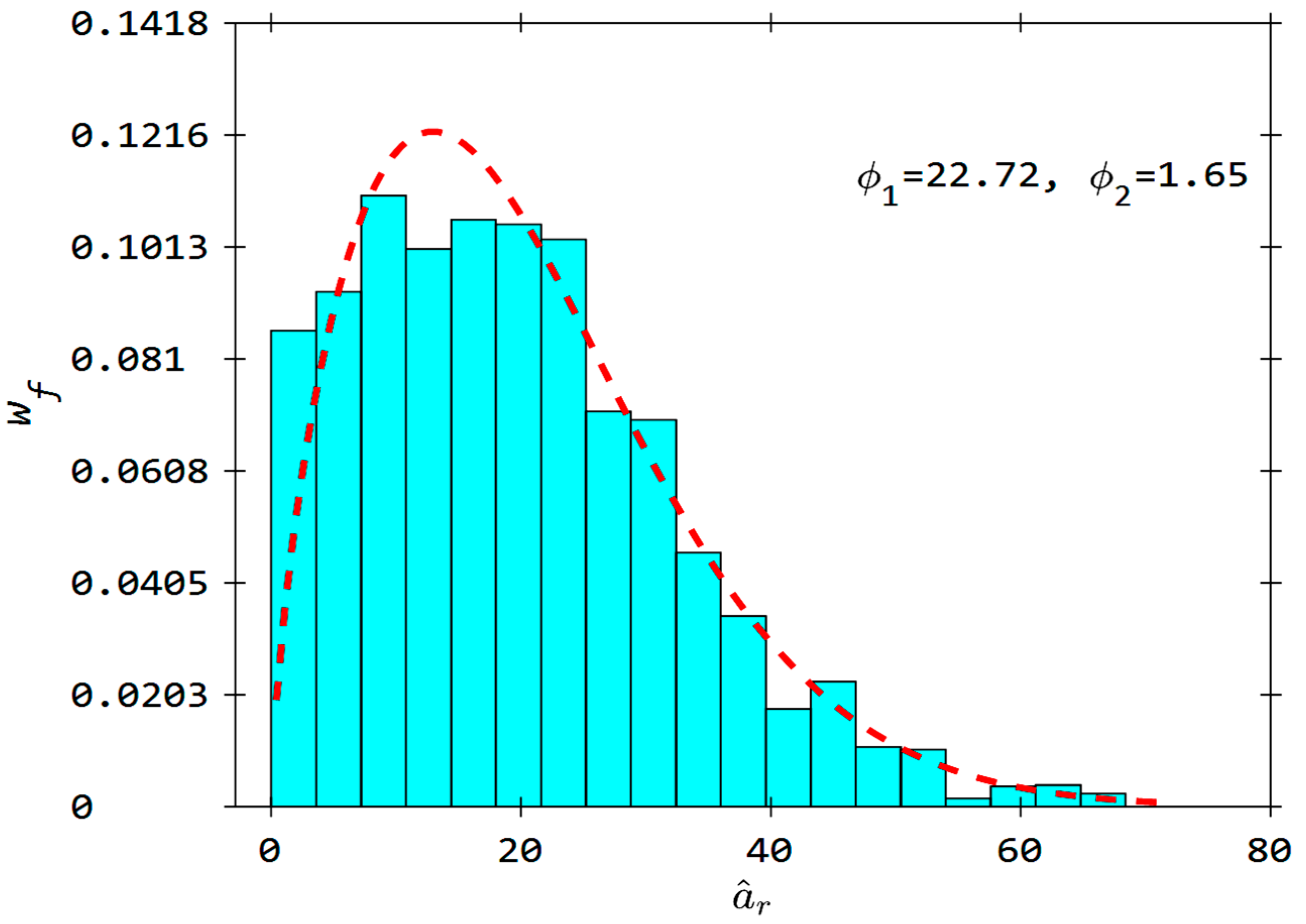
Figure 5.
Fiber aspect ratio distribution extracted for ROI-II. (red dashed line represents the fitted Weibull distribution function curve).
Figure 5.
Fiber aspect ratio distribution extracted for ROI-II. (red dashed line represents the fitted Weibull distribution function curve).
Figure 6.
Isometric view of the deformation contours of RVE-II, #14 from ROI-II, overlayed over the undeformed volume under different loading values: (a) tensile response in -direction; (b) tensile response in -direction; (c) shear response in -plane.
Figure 6.
Isometric view of the deformation contours of RVE-II, #14 from ROI-II, overlayed over the undeformed volume under different loading values: (a) tensile response in -direction; (b) tensile response in -direction; (c) shear response in -plane.
Figure 7.
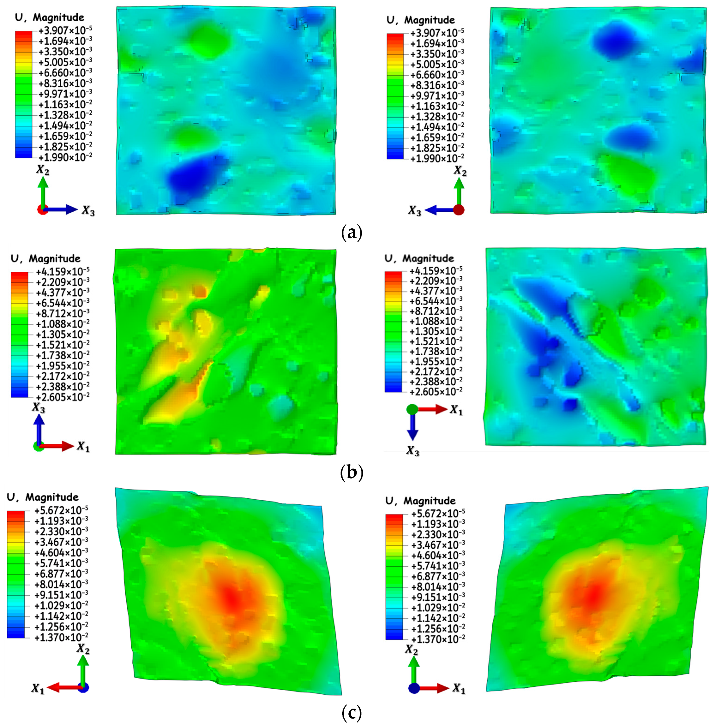
Deformation contours of RVE-II, #14 from ROI-II, showing the topography of opposing bounding face pairs to validate the implementation of PBC for loading in the (a) -direction, (b) -direction and (c) -plane. The images show RVE bounding faces in the negative (left column) and positive (right column) direction (or normal in case of shear) to the direction of the applied loading.
Figure 8.
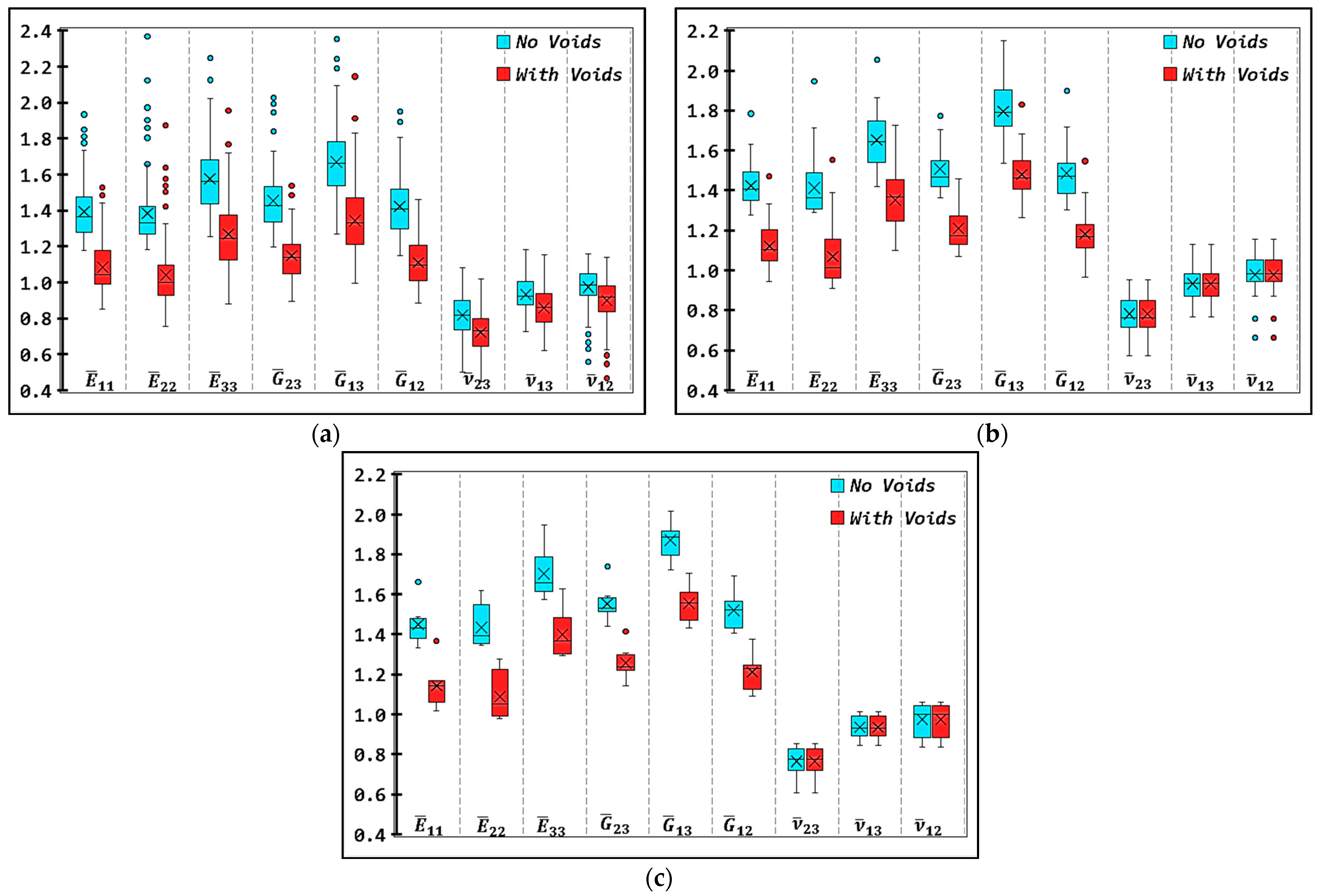
Box plot showing the mean values (‘x’ markers), median values (horizontal lines), interquartile intervals (box limits), extremums (whiskers) and outliers (isolated points) of the computed normalized engineering constants from RVE realization datasets for (a) RVE-I, (b) RVE-II and (c) RVE-III. Results are shown for analysis cases with micro-voids (red) and without micro-voids (blue) present within the bead’s microstructure.
Figure 9.
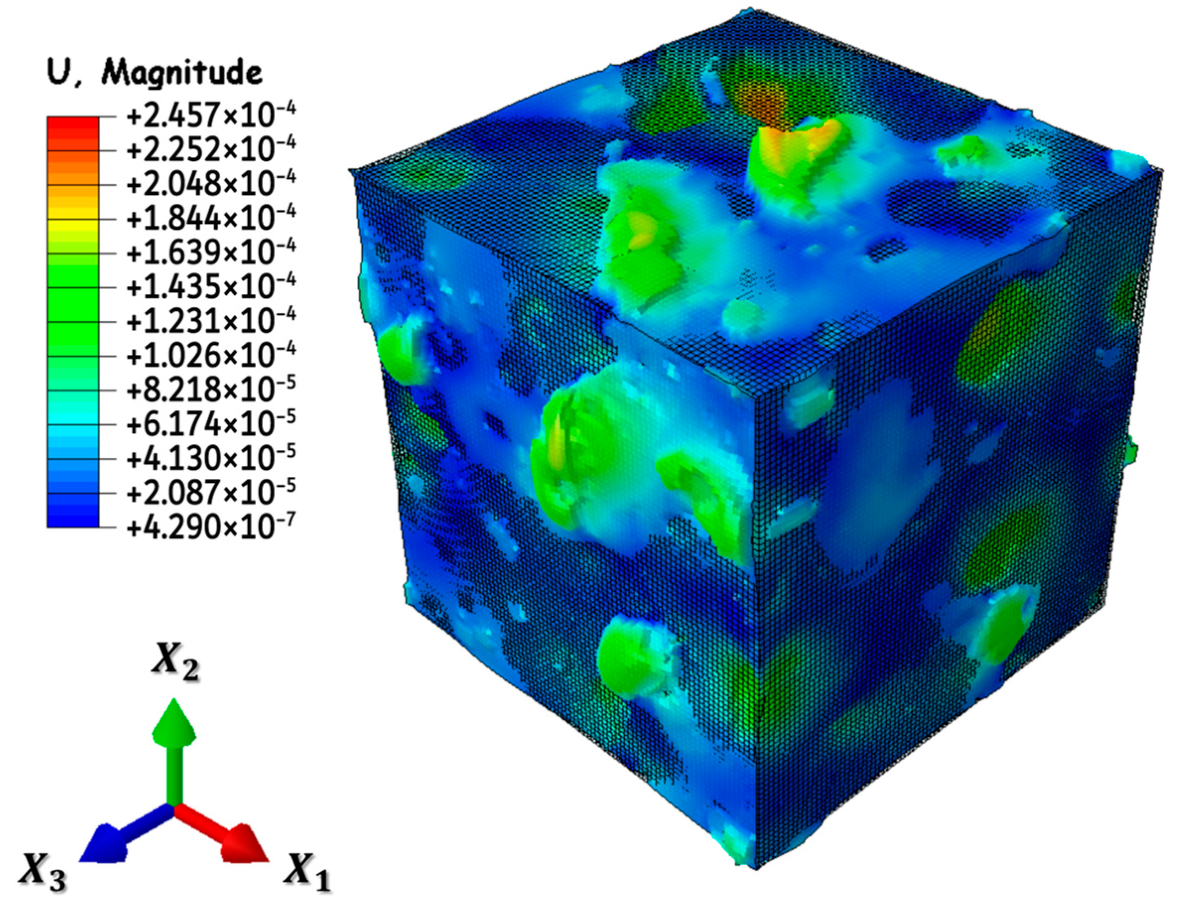
Deformation contour of RVE-II, #14 from ROI-II region, overlayed on the undeformed mesh geometry and showing the bulk response of the volume under thermal load of °C.
Figure 9.
Deformation contour of RVE-II, #14 from ROI-II region, overlayed on the undeformed mesh geometry and showing the bulk response of the volume under thermal load of °C.
Figure 10.
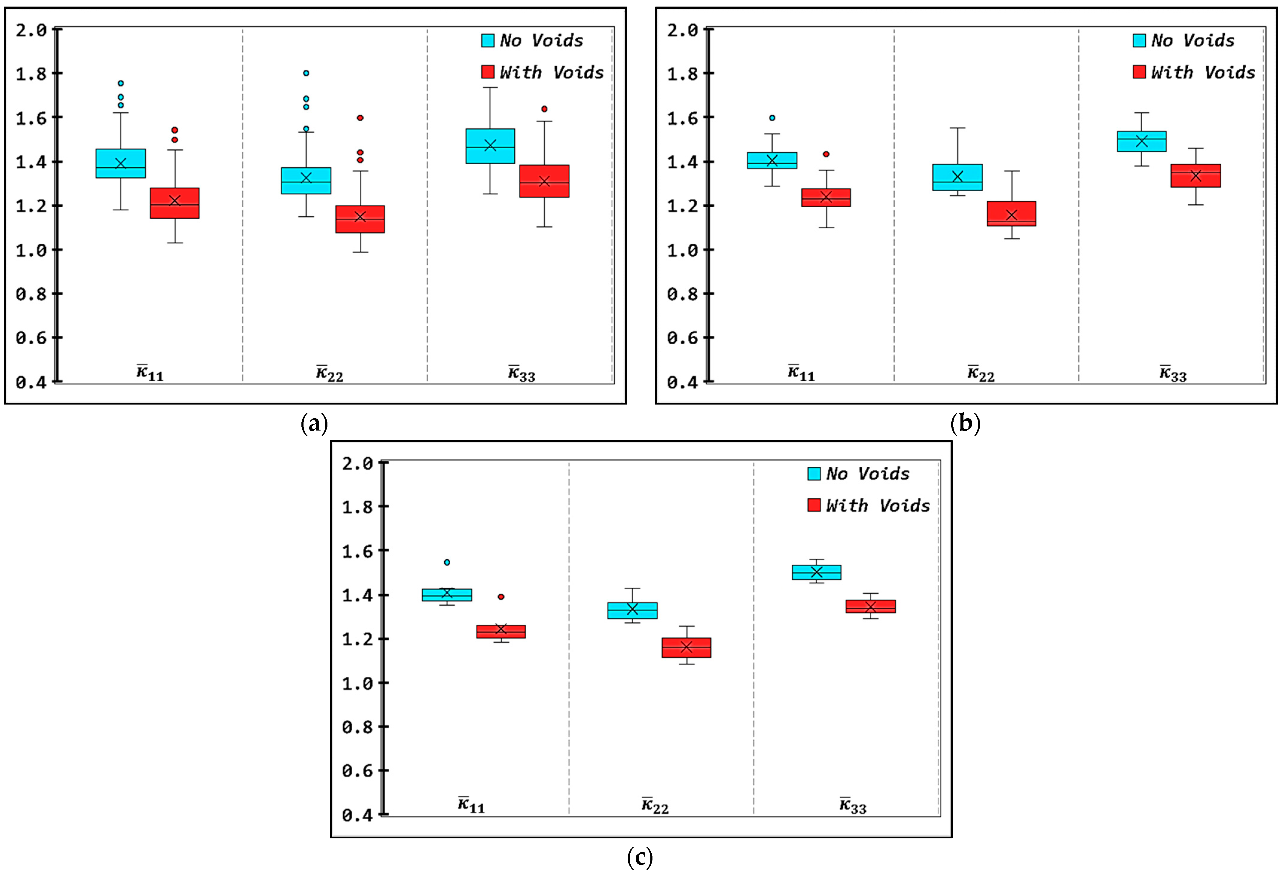
Box plot showing the mean values (‘x’ markers), median values (horizontal lines), interquartile intervals (box limits), extremums (whiskers) and outliers (isolated points) of the computed components of the normalized effective CTE tensor from the RVE realization datasets for (a) RVE-I, (b) RVE-II and (c) RVE-III. Results are shown for analyzed cases with micro-voids (red) and without micro-voids (blue) present within the bead’s microstructure.
Figure 11.
Temperature contours of RVE-II, realization #14 from ROI-II, for three thermal load conditions: (a) thermal gradient in -direction, (b) thermal gradient in -direction and (c) thermal gradient in -direction. Units of in [°C].
Figure 11.
Temperature contours of RVE-II, realization #14 from ROI-II, for three thermal load conditions: (a) thermal gradient in -direction, (b) thermal gradient in -direction and (c) thermal gradient in -direction. Units of in [°C].
Figure 12.
Box plot showing the mean values (‘x’ markers), median values (horizontal lines), interquartile intervals (box limits), extremums (whiskers) and outliers (isolated points) of the diagonal components of the normalized effective TC tensor from the RVE realizations for (a) RVE–I, (b) RVE-II and (c) RVE-III. Results are shown for the analyzed cases with micro-voids (red) and without micro-voids (blue) present within the bead’s microstructure.
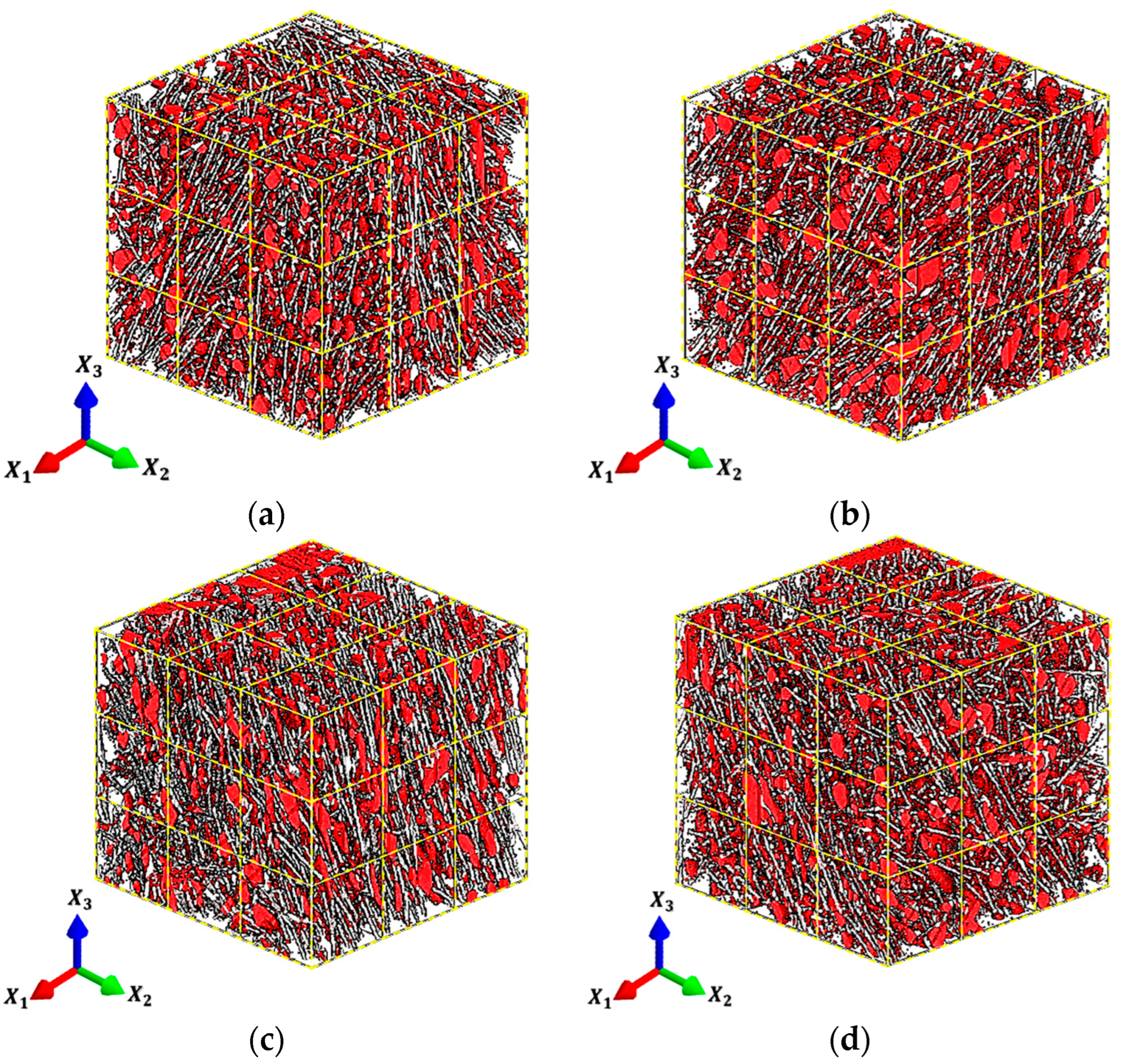
Figure 13.
Three-dimensional µCT volume view showing internal microstructure (fiber—gray; voids—red) of the various ROI volumes and the RVE-II instances for each: (a) ROI-I, (b) ROI-II, (c) ROI-III and (d) ROI-IV.
Figure 13.
Three-dimensional µCT volume view showing internal microstructure (fiber—gray; voids—red) of the various ROI volumes and the RVE-II instances for each: (a) ROI-I, (b) ROI-II, (c) ROI-III and (d) ROI-IV.
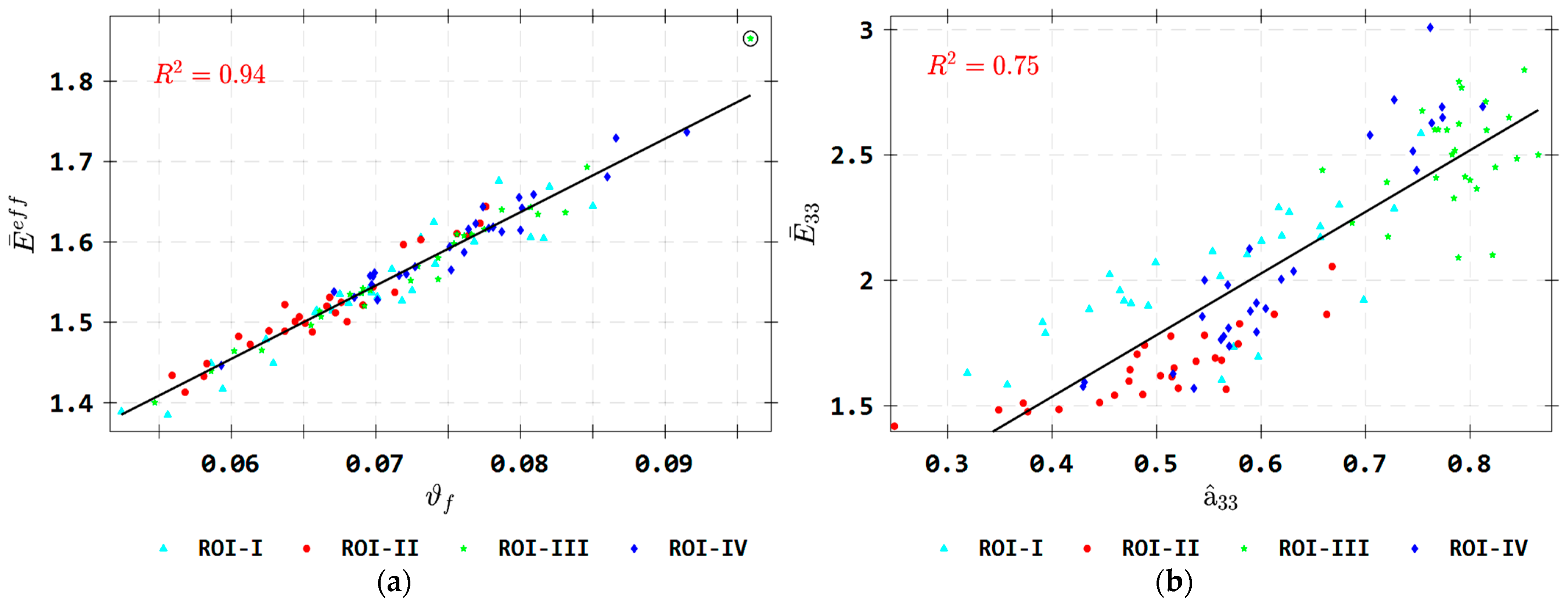
Figure 14.
Linear correlation plots between (a) the effective elastic modulus and the fiber volume fraction and between (b) the elastic modulus component and the average fiber orientation tensor component for non-porous RVE-II instances of the various ROIs. (circled markers indicate outlier datapoints).
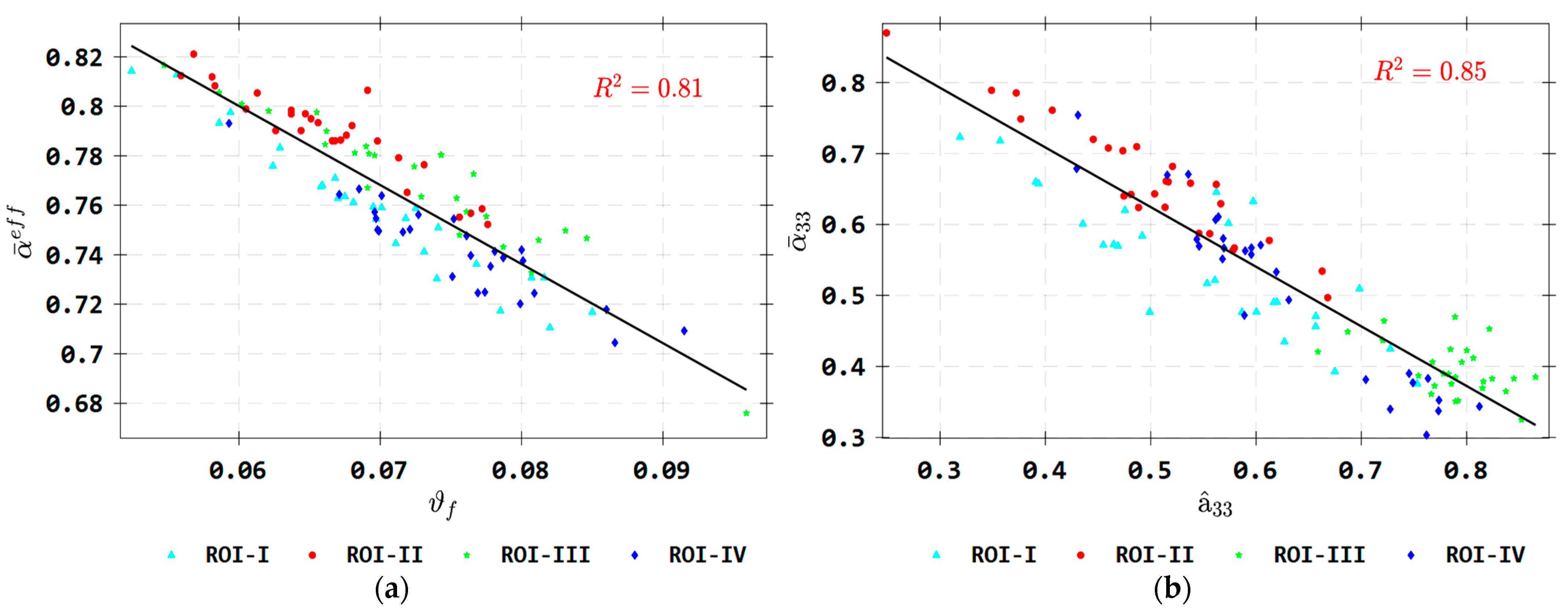
Figure 15.
Linear correlation plots between (a) the apparent ECTE magnitude with the fiber volume fraction and between (b) the ECTE tensor component and the average fiber orientation tensor component for non-porous RVE-II instances of the various ROIs.
Figure 15.
Linear correlation plots between (a) the apparent ECTE magnitude with the fiber volume fraction and between (b) the ECTE tensor component and the average fiber orientation tensor component for non-porous RVE-II instances of the various ROIs.
Figure 16.
Linear correlation plots between (a) the apparent ETC magnitude and the fiber volume fraction and between (b) the ETC tensor component and the average fiber orientation tensor component for non-porous RVE-II instances of the various ROIs. (circled markers indicate outlier datapoints).
Figure 16.
Linear correlation plots between (a) the apparent ETC magnitude and the fiber volume fraction and between (b) the ETC tensor component and the average fiber orientation tensor component for non-porous RVE-II instances of the various ROIs. (circled markers indicate outlier datapoints).
Table 1.
Isotropic properties of the microconstituents of the 13% CF-ABS composite material.
Table 1.
Isotropic properties of the microconstituents of the 13% CF-ABS composite material.
| | | | | | | |
|---|
| | | | |
|---|
| Fiber | 230.0 | 0.20 | −0.61 | 3.060 | 1.76 | 777 |
| Matrix | 2.55 | 0.35 | 90.1 | 0.175 | 1.05 | 1865 |
Table 2.
Mean fiber aspect ratio and fiber length coefficient of variation from all realizations of RVE-I, RVE-II and RVE-III from ROI-II.
Table 2.
Mean fiber aspect ratio and fiber length coefficient of variation from all realizations of RVE-I, RVE-II and RVE-III from ROI-II.
| RVE Size | RVE-I | RVE-II | RVE-III |
|---|
| 8.58 | 12.38 | 15.69 |
| 10.50 | 7.19 | 7.01 |
Table 3.
Computed values of average elastic stiffness for ROI-II region obtained from the numerical (FE) homogenization approach based on RVE-II and the orientation-averaged Mori–Tanaka (MT) method for the 13% CF/ABS SFRP composite (components not shown indicate a zero value).
Table 3.
Computed values of average elastic stiffness for ROI-II region obtained from the numerical (FE) homogenization approach based on RVE-II and the orientation-averaged Mori–Tanaka (MT) method for the 13% CF/ABS SFRP composite (components not shown indicate a zero value).
| Cases | Non-Porous | Porous |
|---|
| FE | | |
| MT | | |
Table 4.
Mean values of engineering elastic constants for ROI-II computed from the numerical FE homogenization schemes for all RVE cases (i.e., RVE-I, II and III, with 125, 27 and 8 realizations, respectively) with non-porous and porous microstructures.
Table 4.
Mean values of engineering elastic constants for ROI-II computed from the numerical FE homogenization schemes for all RVE cases (i.e., RVE-I, II and III, with 125, 27 and 8 realizations, respectively) with non-porous and porous microstructures.
| Cases | RVE | | | | | | | | | |
|---|
| non-porous | I | 1.39 | 1.38 | 1.58 | 1.45 | 1.67 | 1.42 | 0.82 | 0.93 | 0.97 |
| II | 1.42 | 1.41 | 1.65 | 1.51 | 1.79 | 1.49 | 0.78 | 0.93 | 0.98 |
| III | 1.45 | 1.43 | 1.70 | 1.55 | 1.87 | 1.52 | 0.76 | 0.94 | 0.97 |
| porous | I | 1.08 | 1.04 | 1.27 | 1.15 | 1.34 | 1.11 | 0.72 | 0.86 | 0.90 |
| II | 1.12 | 1.07 | 1.35 | 1.21 | 1.48 | 1.18 | 0.78 | 0.93 | 0.98 |
| III | 1.14 | 1.09 | 1.40 | 1.26 | 1.56 | 1.21 | 0.76 | 0.94 | 0.97 |
Table 5.
Mean values and standard deviation of the coefficient of determination for ROI-II computed from the least squares regression fitting procedure for all RVE cases (i.e., RVE-I, II and III).
Table 5.
Mean values and standard deviation of the coefficient of determination for ROI-II computed from the least squares regression fitting procedure for all RVE cases (i.e., RVE-I, II and III).
| Cases | Non-Porous | Porous |
|---|
| RVE | I | II | III | I | II | III |
|---|
| 0.92 | 0.90 | 0.88 | 0.87 | 0.84 | 0.81 |
| 0.05 | 0.05 | 0.05 | 0.08 | 0.07 | 0.08 |
Table 6.
Relative error [%] in the magnitude of the predicted effective elastic modulus, , of ROI-II between the Mori–Tanaka analytical model and numerical FE homogenization schemes for all RVE cases (I, II and III).
Table 6.
Relative error [%] in the magnitude of the predicted effective elastic modulus, , of ROI-II between the Mori–Tanaka analytical model and numerical FE homogenization schemes for all RVE cases (I, II and III).
| Cases | Non-Porous | Porous |
|---|
| RVE | I | II | III | I | II | III |
|---|
| FE | 1.46 | 1.52 | 1.56 | 1.13 | 1.20 | 1.23 |
| MT | 1.31 | 1.41 | 1.47 | 1.08 | 1.16 | 1.22 |
| 10.21 | 8.20 | 5.86 | 4.49 | 3.38 | 1.49 |
Table 7.
Coefficient of variation [%] for the magnitude of the effective elastic modulus, , for all RVE cases (I, II and III) of ROI-II and for both the Mori–Tanaka analytical model and the numerical FE homogenization scheme.
Table 7.
Coefficient of variation [%] for the magnitude of the effective elastic modulus, , for all RVE cases (I, II and III) of ROI-II and for both the Mori–Tanaka analytical model and the numerical FE homogenization scheme.
| Cases | Non-Porous | Porous |
|---|
| RVE | I | II | III | I | II | III |
|---|
| FE | 7.13 | 3.91 | 2.37 | 7.78 | 4.23 | 2.47 |
| MT | 3.54 | 2.18 | 2.12 | 4.17 | 2.26 | 2.39 |
Table 8.
Mean values of the diagonal components of the effective CTE tensor for all RVE cases (I, II and III) of ROI-II computed using numerical FE homogenization.
Table 8.
Mean values of the diagonal components of the effective CTE tensor for all RVE cases (I, II and III) of ROI-II computed using numerical FE homogenization.
| Cases | Non-Porous | Porous |
|---|
| RVE | | | | | | |
|---|
| I | 0.83 | 0.91 | 0.70 | 0.81 | 0.89 | 0.67 |
| II | 0.82 | 0.90 | 0.66 | 0.79 | 0.88 | 0.63 |
| III | 0.81 | 0.89 | 0.64 | 0.79 | 0.87 | 0.61 |
Table 9.
Computed normalized and the associated relative error [%] in the computed effective CTE magnitude of ROI-II between the numerical FE homogenized results and the Mori–Tanaka (MT) analytical results for all RVE sizes (RVE-I, II and III).
Table 9.
Computed normalized and the associated relative error [%] in the computed effective CTE magnitude of ROI-II between the numerical FE homogenized results and the Mori–Tanaka (MT) analytical results for all RVE sizes (RVE-I, II and III).
| Cases | Non-Porous | Porous |
|---|
| RVE | I | II | III | I | II | III |
|---|
| FE | 0.81 | 0.79 | 0.78 | 0.79 | 0.76 | 0.75 |
| MT | 0.85 | 0.82 | 0.79 | 0.84 | 0.81 | 0.79 |
| 5.45 | 3.85 | 2.00 | 7.02 | 6.07 | 4.59 |
Table 10.
Coefficient of variation [%] for the normalized effective CTE magnitude ( for all RVE cases (I, II and III) of ROI-II and for the Mori–Tanaka analytical model and the numerical FE homogenization schemes.
Table 10.
Coefficient of variation [%] for the normalized effective CTE magnitude ( for all RVE cases (I, II and III) of ROI-II and for the Mori–Tanaka analytical model and the numerical FE homogenization schemes.
| Cases | Non-Porous | Porous |
|---|
| RVE | I | II | III | I | II | III |
|---|
| FE | 4.00 | 2.28 | 1.12 | 5.36 | 3.16 | 1.61 |
| MT | 2.89 | 1.86 | 1.91 | 3.23 | 2.03 | 1.99 |
Table 11.
Mean values of effective TCs for all RVE cases (RVE-I, I and III) for ROI-II computed with the numerical FE homogenization scheme.
Table 11.
Mean values of effective TCs for all RVE cases (RVE-I, I and III) for ROI-II computed with the numerical FE homogenization scheme.
| Cases | Non-Porous | Porous |
|---|
| RVE | | | | | | |
|---|
| I | 1.39 | 1.32 | 1.47 | 1.22 | 1.15 | 1.31 |
| II | 1.40 | 1.33 | 1.49 | 1.24 | 1.16 | 1.33 |
| III | 1.41 | 1.33 | 1.50 | 1.24 | 1.16 | 1.35 |
Table 12.
Relative error [%] in the predicted effective TC magnitude ( for ROI-II between the numerical FE homogenization scheme and the Mori–Tanaka (MT) analytical results for all RVE sizes (RVE-I, II and III).
Table 12.
Relative error [%] in the predicted effective TC magnitude ( for ROI-II between the numerical FE homogenization scheme and the Mori–Tanaka (MT) analytical results for all RVE sizes (RVE-I, II and III).
| Cases | Non-Porous | Porous |
|---|
| RVE | I | II | III | I | II | III |
|---|
| FE | 1.40 | 1.41 | 1.42 | 1.23 | 1.24 | 1.25 |
| MT | 1.35 | 1.38 | 1.40 | 1.18 | 1.22 | 1.24 |
| 3.48 | 1.79 | 0.98 | 3.46 | 1.95 | 1.16 |
Table 13.
Coefficient of variation [%] for the predicted normalized apparent ETC ( of ROI-II for both the Mori–Tanaka analytical model and the numerical FE homogenization schemes and for all RVE cases (I, II and III).
Table 13.
Coefficient of variation [%] for the predicted normalized apparent ETC ( of ROI-II for both the Mori–Tanaka analytical model and the numerical FE homogenization schemes and for all RVE cases (I, II and III).
| Cases | Non-Porous | Porous |
|---|
| RVE | I | II | III | I | II | III |
|---|
| FE | 5.63 | 2.92 | 1.78 | 5.49 | 2.80 | 1.83 |
| MT | 4.85 | 2.59 | 1.83 | 4.86 | 2.47 | 1.93 |
