Three-Dimensional Thermoelastic Contact Model of Coated Solids with Frictional Heat Partition Considered

Abstract

In this paper, a three-dimensional thermoelastic contact model of coated solids with the frictional heat partition considered is developed by introducing a frictional heat partition model. The influence coefficients of the temperature rise, normal displacement and stress components in the three-dimensional thermoelastic contact model are converted from their corresponding frequency response functions (FRFs) with a conversion method based on the fast Fourier transform (FFT), and the FRFs of solids coated with a homogeneous coating subjected to a coupled action of the mechanical loading and the frictional heat flux on its surface are deduced in the frequency domain by introducing a two-dimensional Fourier integral transform. The contact pressure and the frictional heat partition between the two bodies are solved by employing a fast numerical algorithm based on the conjugate gradient method (CGM) and a discrete convolution fast Fourier transformation (DC-FFT). Comparison between the solutions of the present model and those of a thermoelastic contact model in literature is conducted in order to validate the present model. Several specific conclusions on the effect of the sliding speed, thermoelastic properties and thickness of the coating are drawn based on the result of numerical investigation by utilizing the present model.

1. Introduction

Solid coatings, such as TiN, diamond-like-carbon (DLC) and MoS₂, are widely employed to improve the tribological performance and service life of tribo-parts [1,2,3]. More and more tribo-parts, such as gears, bearings, are coated for anti-scuffing, anti-friction and anti-wear, especially those working under severe performance conditions. A three-dimensional thermoelastic contact model of coated solids is essential for a more accurate analysis of the contact behavior by considering the partition of frictional heat between the bodies in contact, since the thermal effect of the frictional heat can exert a significant impact on the contact behavior [4].

In the theoretical analysis of the mechanics of solids, linear elastic theory uses various integral transform techniques to produce solutions [5]. The general theory of the stress and displacement of layered systems was structured by Burmister for analyzing the contact under prescribed axially symmetric surface normal loading [6,7]. Chen [8,9] extended the applications to both axisymmetric and non-axisymmetric normal surface loading. O’Sullivian and King [10] studied the contact of layered materials using Papkovich–Neuber potentials. Nogi and Kato [11] improved the computing speed by employing the fast Fourier transform (FFT) technique based on the work of O’Sullivian and King. The Papkovich–Neuber potentials were further employed to study the sliding contact or partial slip contact problem for solids coated with a monolayer or multilayers [12,13,14]. Wang et al. [15] also adopted Papkovich–Neuber potentials to conduct a systematic investigation of the effect of the thickness and stiffness of a homogeneous coating on the contact behavior under various friction coefficients. It was also reported that the equivalent inclusion method, which was often employed to analyze the contact concerning inhomogeneities, also can be used to analyze the contact of coated solids [16]. Kral and Komvopoulos [17,18] employed the finite element method (FEM) to study the contact of elastic-plastic layered mediums subjected to repeated indentations by a rigid sphere. Kang et al. [19] also adopted FEM to analyze the failure mechanism of plasma sprayed AT40 coatings under different rolling-sliding contact conditions. Besides the research work mentioned above, numerous investigations have also been conducted on the problem of solids with a homogeneous layer subjected to the mechanical loading coupling with the thermal heat flux, as well as that of uncoated solids [20,21,22,23,24]. Leroy et al. [25,26] applied the Fourier integral transform to a finite thickness layered medium subjected to a moving line heat source and obtained a system of equations which links the transformed quantities, and the solution in the space domain by applying the inverse FFT. Ju and Farris [27] deduced an FFT thermoelastic solution for a half plane subjected to a moving heat flux. Shodja and Ghahremaninejad [28], Ke and Wang [29] studied the problem of a half plane coated with an functionally gradient material (FGM) layer subjected to the coupled action of the mechanical loading and the thermal heat flux. Shi et al. [30] investigated the thermal elastic field of a half space with multilayers using the Fourier integral transform. However, in those studies, the heat flux was given by hypothesis rather than a partition model, and the effect of the thermal displacement on the contact pressure was not considered. The FEM was also used to analyze the contact problem of coated solids subjected to the coupled action of the mechanical loading and the thermal heat flux. Kulkarni et al. [31] established a two-dimensional FEM model for the thermoelastoplastic contact under repeated translation loading. Komvopoulos et al. [32,33] developed a three-dimensional FEM model of elasto-plastic layered mediums under the coupled action of the mechanical loading and the thermal heat flux. In the last several decades, meaningful studies have been done on the contact problem of coated solids and efforts have been made to develop a design and optimization technology of coating for improving the performance of anti-wear, anti-friction and fatigue strength etc. [34,35,36,37]. However, little attention has been paid to the investigation of the contact problem of coated solids considering the frictional heat partition, which should be one of the essential factors in the contact problem.

In this paper, a three-dimensional thermoelastic contact model of coated solids considering the partition of frictional heat is developed by introducing a frictional heat partition model. The influence coefficients (ICs) of the temperature rise, surface normal displacement and stress components are converted from their corresponding frequency response functions (FRFs) by employing a numerical conversion method based on the FFT, and the FRFs of the temperature rise, displacement and stress components of a solid with a homogenous coating subjected to the mechanical loading coupling with the frictional heat flux are derived and given in explicit formulas. A fast iteration algorithm based on the conjugate gradient method (CGM) and a discrete convolution fast Fourier transformation (DC-FFT) are adopted to obtain the contact pressure, heat partition and stress in the subsurface. The present model is validated by a comparison between the solution of the present model and that of a model in literature. Lastly, a numerical investigation of the effect of the sliding speed, thermoelastic properties and thickness of the coating on the contact behavior is further conducted.

2. Theory

2.1. Contact Model

According to the authors of [38], the thermoelastic contact model of an elastic ball brought into sliding contact with a half space with a homogeneous coating subjected to an external normal load W, as shown in Figure 1, can be described as follows:

$$\begin{array}{r}g(x,y)=0,p(x,y)>0\forall (x,y)\in {\Omega }_c\\ g(x,y)>0,p(x,y)=0\forall (x,y)\notin {\Omega }_c\\ {\displaystyle {\int }_{-\infty }^{+\infty }{\displaystyle {\int }_{-\infty }^{+\infty }p(x,y)dxdy}}=W\\ g(x,y)=g_o(x,y)+u_e(x,y)+u_t(x,y)-\mathsf{\delta }\end{array}$$

(1)

where g is the gap between the surfaces of the two bodies in contact after the external normal load W is applied, g₀ is the initial gap before the external normal load W is applied, p is the contact pressure between the two bodies, u_e is the surface normal displacement due to the contact pressure, u_t is the surface normal displacement due to the frictional heat flux, δ is the normal approach and Ω_c represents the real contact area.

In order to employ numerical methods to solve the contact model, a square calculation domain $\Omega =\left\{(x,y)|-2a_{\mathrm{H}}\le x\le 2a_{\mathrm{H}},-2a_{\mathrm{H}}\le y\le 2a_{\mathrm{H}}\right\}$ is selected and uniformly divided into N_x × N_y surface square elements centered on the grid nodes. Here a_H is the contact radius of the substrate material in Hertz point contact, N_x and N_y are the numbers of elements in x and y direction respectively. The contact pressure distribution is approximated by a piecewise constant function that is uniform within each surface element. Then the Equation (1) can be converted into a discretized form:

$$\begin{array}{r}g[i,j]=0,p[i,j]>0\forall [i,j]\in {\Omega }_c\\ g[i,j]>0,p[i,j]=0\forall [i,j]\notin {\Omega }_c\\ \Delta x\Delta y{\displaystyle \sum _{i=0}^{N_x-1}{\displaystyle \sum _{j=0}^{N_y-1}p[i,j]}}=W\\ g[i,j]=g_o[i,j]+u_e[i,j]+u_t[i,j]-\mathsf{\delta }\end{array}$$

(2)

where Δx and Δy are the discretization sizes in x and y direction respectively.

According to the linear superposition principle, the displacements u_e and u_t are obtained by:

$${\mathrm{u}}_e[i,j]={\displaystyle \sum _{k=1}^2{\displaystyle \sum _{r=0}^{N_x-1}{\displaystyle \sum _{s=0}^{N_y-1}K{N}_k[i-r,j-s]}}}p[r,s]$$

(3)

$${\mathrm{u}}_t[i,j]={\displaystyle \sum _{k=1}^2{\displaystyle \sum _{r=0}^{N_x-1}{\displaystyle \sum _{s=0}^{N_y-1}K{Q}_k[i-r,j-s]}}}{Q}_k[r,s]$$

(4)

where KN_k[i − r, j − s] and KQ_k[i − r, j − s] are the ICs of the surface normal displacement due to the contact pressure and the surface heat flux respectively, k = 1 and k = 2 represent the elastic ball and the coated solid, respectively.

The overall flow chart of the numerical algorithm is shown in Figure 2a. One solver named NCS in Figure 2a is a normal contact solver for determining the normal contact pressure with a known u_t in Equation (2), the other solver named HPS is a heat partition solver for determining the heat flux of Q₁ and Q₂ within the calculation domain based on a heat partition model seen below in the current section. Several different iteration schemes have been proposed for the solver NCS, and the iteration scheme based on the CGM [39,40] is employed here for its comparatively high rate of convergence and explicit iteration format, which makes it compatible with the fast multi-summation method, namely, the DC-FFT [41].

After the contact pressure and the heat flux applied on the surface of coated solids have been obtained, the stress components and the temperature rise in the subsurface of coated solids can be obtained by:

$$\begin{array}{r}{\mathsf{\sigma }}_{mn}(i,j,z)={\displaystyle \sum _{r=0}^{N_x-1}{\displaystyle \sum _{s=0}^{N_y-1}S{N}_{mn}[i-r,j-s,z]p[r,s]}}+{\displaystyle \sum _{r=0}^{N_x-1}{\displaystyle \sum _{s=0}^{N_y-1}S{T}_{mn}[i-r,j-s,z]q[r,s]}}\\ +{\displaystyle \sum _{r=0}^{N_x-1}{\displaystyle \sum _{s=0}^{N_y-1}S{Q}_{mn}[i-r,j-s,z]Q_2[r,s]}}\\ (mn=zz,yy,xx,xz,yz,xy)\end{array}$$

(5)

$$T_2(i,j,z)={\displaystyle \sum _{r=0}^{N_x-1}{\displaystyle \sum _{s=0}^{N_y-1}T{R}_2[i-r,j-s,z]Q_2[r,s]}}$$

(6)

where SN_mn[i − r, j − s, z], ST_mn[i − r, j − s, z], SQ_mn[i − r, j − s, z] and TR₂[i − r, j − s, z] are the stress components and temperature rise influence coefficients of point at z depth lying directly below the grid node [i, j] for the normal force p, tangential traction q, and heat flux Q₂ applied on the surface element [r, s] of coated solids, respectively. According to the Coulomb’s friction law, the tangential traction q[r, s] is given as follows:

$$q[r,s]={\mathsf{\mu }}_{f}p[r,s]$$

(7)

where μ_f is the frictional coefficient.

In Equations (3)–(6), the surface heat fluxes Q₁ and Q₂ should be determined with a consideration of the frictional heat partition between the two bodies in contact. For simplicity, the previous work [42,43] assumed that the frictional heat flux is solely absorbed by one body or evenly partitioned between the two bodies in contact regardless of the real surface temperature distribution. Blok [44] proposed a frictional heat partition model by matching the maximum flash temperature of the two bodies, which has been adopted by Tian and Kennedy [45]. Jaeger [46] proposed a heat partition model by matching the average temperature within the contact zone instead of matching the maximum temperature, which was adopted by Archard and Rowntree [47]. Francis [48] also proposed a heat partition model by holding the interfacial temperature as the harmonic mean of the two surface temperatures when each body receives all of the frictional heat flux. Gao et al. [49] determined the heat partition between the two bodies by matching the temperature in the whole simulation domain. In the present model, the heat partition model shown as Equation (8), which is established by matching the temperature within the real contact area and has been employed by Bos and Moes [50], Chen and Wang [4], is adopted to determine the frictional heat partition, in which the heat convection and thermal radiation are ignored:

$$\begin{array}{r}({\overline{T}}_1+{\overline{T}}_1[i,j])-({\overline{T}}_2+{\overline{T}}_2[i,j])=0,Q_1[i,j]+Q_2[i,j]=Q[i,j]\forall [i,j]\in {\Omega }_c\\ Q_1[i,j]=Q_2[i,j]=0\forall [i,j]\in {\Omega }_c\end{array}$$

(8)

where ${\overline{T}}_1$ and ${\overline{T}}_2$ are the bulk temperatures of the elastic ball and the coated solid respectively, T₁ and T₂ are the surface temperature rises of the two bodies due to the frictional heat flux, Q₁ and Q₂ are the surface heat fluxes of the two bodies, and Q is the frictional heat flux. The frictional heat flux is as follows:

$$Q[i,j]=V_{s}q[i,j]$$

(9)

where V_s is the sliding speed. Here the heat partition coefficient H_pc is defined to describe the ratio between the heat flux flowing into the coated solid and the total frictional heat flux, shown as Equation (10).

$$H_{pc}={\displaystyle \sum _{i=0}^{N_x-1}{\displaystyle \sum _{j=0}^{N_y-1}{Q}_2[i,j]}}/{\displaystyle \sum _{i=0}^{N_x-1}{\displaystyle \sum _{j=0}^{N_y-1}Q[i,j]}}$$

(10)

The surface temperature rise T_k[i, j] can be obtained by:

$$T_k[i,j]={\displaystyle \sum _{i=0}^{N_x-1}{\displaystyle \sum _{j=0}^{N_y-1}K{T}_k[i-r,j-s]Q_k[r,s]\begin{array}{cc}& \end{array}}}(k=1,2)$$

(11)

where KT_k[i − r, j − s] is the ICs of the surface temperature rise at the grid node [i, j] due to the surface heat flux Q_k[r, s].

By substituting Equation (11) into the Equation (8), the heat partition model can be rewritten as follows:

$$\begin{array}{r}{\displaystyle \sum _{i=0}^{N_x-1}{\displaystyle \sum _{j=0}^{N_y-1}(K{T}_1\left[i-r,j-s\right]+K{T}_2\left[i-r,j-s\right])Q_2\left[i,j\right]=({\overline{T}}_1-{\overline{T}}_2)+}}{\displaystyle \sum _{i=0}^{N_x-1}{\displaystyle \sum _{j=0}^{N_y-1}KT1\left[i-r,j-s\right]Q\left[i,j\right]\forall }}\left[i,j\right]\in \Omega c\\ Q_2\left[i,j\right]=0\forall \left[i,j\right]\in \Omega c\end{array}$$

(12)

The bulk temperatures ${\overline{T}}_1$ and ${\overline{T}}_2$ in Equation (12) can be input according to practical conditions and it is assumed that ${\overline{T}}_1$ equals to ${\overline{T}}_2$ in this paper for simplicity. The unknown Q₂[i, j] in Equation (12) can be solved by a modified iterative algorithm based on a standard CGM [51]. The detail of the modified iterative algorithm can be found in Figure 2b, its difference from the iterative algorithm of a standard CGM can be summarized as follows:

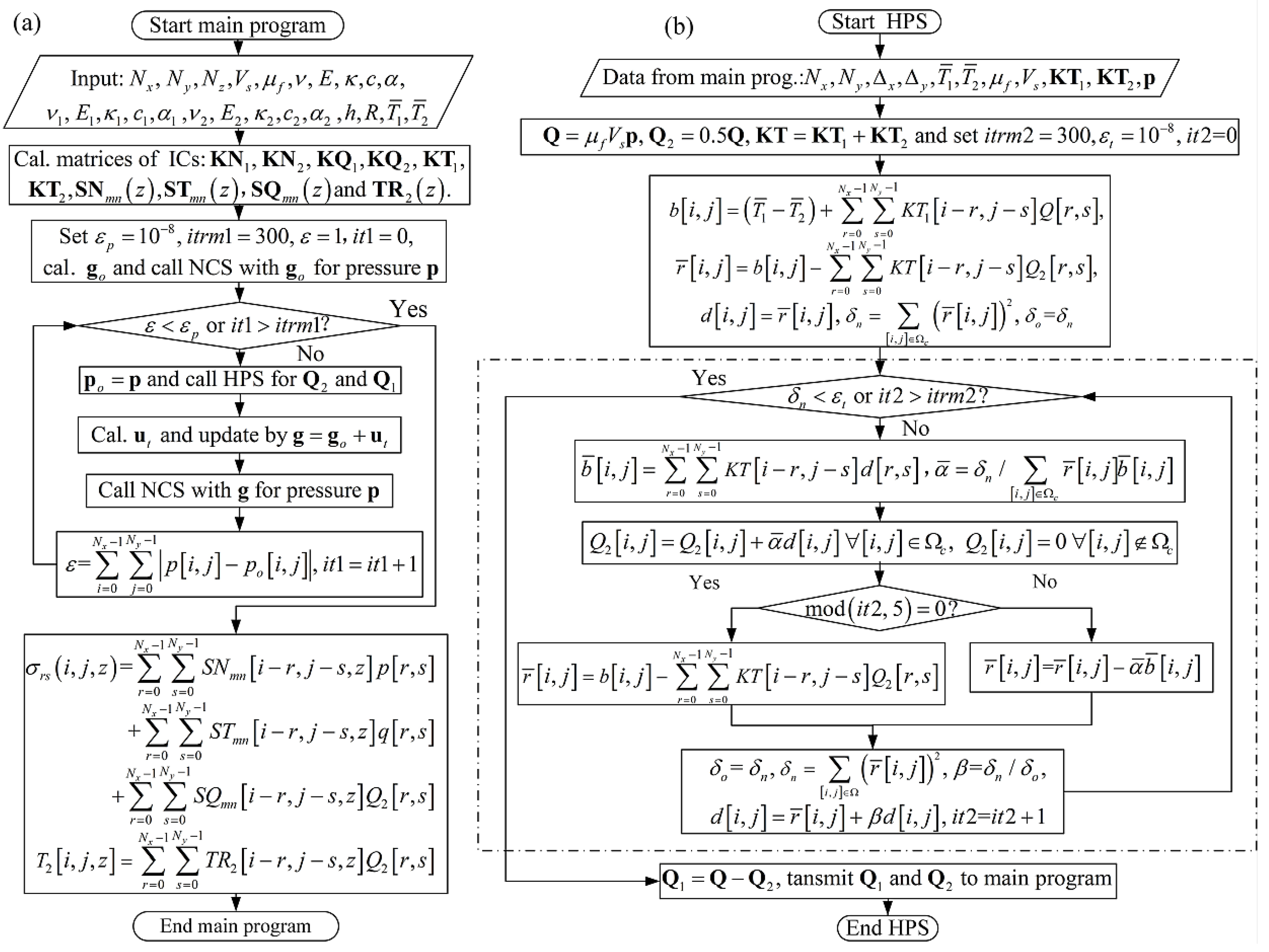
• In the modified iterative algorithm, the calculations of the iteration parameter δ_n and the update length of heat flux $\overline{\mathsf{\alpha }}$ in the conjugate gradient direction are conducted over the real contact area Ω_c rather than the whole calculation domain Ω as follows:

  $$\mathsf{\delta }n={\displaystyle \sum _{[i,j]\in \Omega c}^{}\overline{r}}{[i,j]}^2$$

  (13)

  $$\overline{\mathsf{\alpha }}=\mathsf{\delta }n/{\displaystyle \sum _{[i,j]\in \Omega c}^{}\overline{r}}[i,j]\overline{b}[i,j]$$

  (14)

  where $\overline{r}[i,j]$ and $\overline{b}[i,j]$ are intermediate variables used by the flow chart of heat partition solver as shown in Figure 2b. In the standard CGM, the calculations of δ_n and $\overline{\mathsf{\alpha }}$ are conducted over the whole calculation domain Ω.
• The update of the heat flux Q₂[i, j] is performed only within the real contact area Ω_c in the conjugate gradient direction with the update length $\overline{\mathsf{\alpha }}$. Outside the real contact area Ω_c, the heat flux Q₂[i, j] is enforced to be zero.

For the elastic ball, the ICs of its displacement and stress components due to the mechanical loading are obtained by applying Boussinesq and Cerruti solutions [52]. However, the explicit formulas for all ICs of the coated solid are unavailable as well as the ICs of the elastic ball due to the surface heat flux. In this paper, these ICs are converted from their corresponding FRFs by a numerical conversion method based on FFT [53,54]. The detailed steps of the numerical conversion method adopted in this paper can be found in [15].

2.2. Frequency Response Functions

For solids with a homogeneous coating subjected to the coupled action of the mechanical loading and the frictional heat flux, including the normal pressure, tangential traction and frictional heat flux moving on its surface, as shown in Figure 3, the governing differential equations of the temperature rise and thermoelastic field can be given as Equations (15)–(18) for quasi-static states:

$$\frac{{\partial }^2{T}^{(k)}}{\partial x^2}+\frac{{\partial }^2{T}^{(k)}}{\partial y^2}+\frac{{\partial }^2{T}^{(k)}}{\partial z_k{}^2}=-\frac{V}{{\mathsf{\gamma }}_k}\frac{\partial T^{(k)}}{\partial x}$$

(15)

$$\frac{1}{(1-2{\mathsf{\nu }}_k)}(\frac{{\partial }^2{u}_x^{(k)}}{\partial x^2}+\frac{{\partial }^2{u}_y^{(k)}}{\partial x\partial y}+\frac{{\partial }^2{u}_z^{(k)}}{\partial x\partial z_k})+(\frac{{\partial }^2{u}_x^{(k)}}{\partial x^2}+\frac{{\partial }^2{u}_x^{(k)}}{{\partial }^{2}y}+\frac{{\partial }^2{u}_x^{(k)}}{\partial z_k{}^2})=\frac{2(1+{\mathsf{\nu }}_k){\mathsf{\alpha }}_k}{(1-2{\mathsf{\nu }}_k)}\partial T^{(k)}/\partial x$$

(16)

$$\frac{1}{(1-2{\mathsf{\nu }}_k)}(\frac{{\partial }^2{u}_x^{(k)}}{\partial x\partial y}+\frac{{\partial }^2{u}_y^{(k)}}{\partial y^2}+\frac{{\partial }^2{u}_z^{(k)}}{\partial y\partial z_k})+(\frac{{\partial }^2{u}_y^{(k)}}{\partial x^2}+\frac{{\partial }^2{u}_y^{(k)}}{\partial y^2}+\frac{{\partial }^2{u}_y^{(k)}}{\partial z_k{}^2})=\frac{2(1+{\mathsf{\nu }}_k){\mathsf{\alpha }}_k}{(1-2{\mathsf{\nu }}_k)}\partial T^{(k)}/\partial y$$

(17)

$$\frac{1}{(1-2{\mathsf{\nu }}_k)}(\frac{{\partial }^2{u}_x^{(k)}}{\partial x\partial z_k}+\frac{{\partial }^2{u}_y^{(k)}}{\partial y\partial z_k}+\frac{{\partial }^2{u}_z^{(k)}}{\partial z_k{}^2})+(\frac{{\partial }^2{u}_z^{(k)}}{{\partial }^{2}x}+\frac{{\partial }^2{u}_z^{(k)}}{\partial y^2}+\frac{{\partial }^2{u}_z^{(k)}}{\partial z_k{}^2})=\frac{2(1+{\mathsf{\nu }}_k){\mathsf{\alpha }}_k}{(1-2{\mathsf{\nu }}_k)}\partial T^{(k)}/\partial z_k$$

(18)

where T is the temperature rise, u is the displacement, V is the moving speed of the mechanical loading and the heat flux, and ν, γ and α represent the Poisson ratio, thermal diffusivity and thermal expansion coefficient respectively. The thermal diffusivity is the thermal conductivity κ divided by the volumetric heat capacity c, and the volumetric heat capacity c is a product of the density and the specific heat capacity.

Analogous to the method employed in [55], a two-dimensional Fourier integral transform

$$\tilde{\Phi }={\displaystyle {\int }_{-\infty }^{\infty }{\displaystyle {\int }_{-\infty }^{\infty }\Phi {\mathrm{e}}^{-\mathrm{i}({\mathsf{\omega }}_{x}x+{\mathsf{\omega }}_{y}y)}}\mathrm{d}x\mathrm{d}y}$$

and two intermediate functions $F^{(k)}=\partial u_x^{(k)}/\partial y-\partial u_y^{(k)}/\partial x$, $G^{(k)}=\partial u_x^{(k)}/\partial x+\partial u_y^{(k)}/\partial y$ are introduced, then Equations (15)–(18) can be rewritten as follows:

$$\frac{{\partial }^2{\tilde{T}}^{(k)}}{\partial z_k{}^2}-\left({\mathsf{\omega }}^2-i{\mathsf{\omega }}_x\frac{V}{{\mathsf{\gamma }}_k}\right){\tilde{T}}^{(k)}=0$$

(19)

$$\frac{{\partial }^2{\tilde{F}}^{(k)}}{\partial z_k{}^2}-{\mathsf{\omega }}^2{\tilde{F}}^{(k)}=0$$

(20)

$$\frac{{\partial }^2{\tilde{G}}^{(k)}}{\partial z_k{}^2}-{\mathsf{\omega }}^2(d^{(k)}+1){\tilde{G}}^{(k)}-{\mathsf{\omega }}^2{d}^{(k)}\frac{\partial {\tilde{u}}_z^{(k)}}{\partial z_k}=-K^{(k)}{\mathsf{\omega }}^2{\tilde{T}}^{(k)}$$

(21)

$$(1+d^{(k)})\frac{{\partial }^2{\tilde{u}}_z^{(k)}}{\partial z_k{}^2}-{\mathsf{\omega }}^2{\tilde{u}}_k^{(k)}+d^{(k)}\frac{\partial {\tilde{G}}^{(k)}}{\partial z_k}=K^{(k)}\frac{\partial {\tilde{T}}^{(k)}}{\partial z_k}$$

(22)

where $d^{(k)}=1/(1-2{\mathsf{\nu }}_k)$, $K^{(k)}=2(1+{\mathsf{\nu }}_k){\mathsf{\alpha }}_k/(1-2{\mathsf{\nu }}_k)$, $\mathsf{\omega }=\sqrt{{\mathsf{\omega }}_x{}^2+{\mathsf{\omega }}_y{}^2}$, $i=\sqrt{-1}$.

The general solutions of ${\tilde{T}}^{(k)}$, ${\tilde{u}}_z{}^{(k)}$, ${\tilde{G}}^{(k)}$ and ${\tilde{F}}^{(k)}$ can be deduced as follows:

$${\tilde{T}}^{(k)}=M_1^{(k)}{\mathrm{e}}^{-r^{(k)}{z}_k}+M_2^{(k)}{\mathrm{e}}^{r^{(k)}{z}_k}$$

(23)

$${\tilde{F}}^{(k)}=A_1^{(k)}{\mathrm{e}}^{-\mathsf{\omega }{z}_k}+A_2^{(k)}{\mathrm{e}}^{\mathsf{\omega }{z}_k}$$

(24)

$${\tilde{u}}_z^{(k)}=B_1^{(k)}{\mathrm{e}}^{-\mathsf{\omega }{z}_k}+B_2^{(k)}{z}_k{\mathrm{e}}^{-\mathsf{\omega }{z}_k}+B_3^{(k)}{\mathrm{e}}^{\mathsf{\omega }{z}_k}+B_4^{(k)}{z}_k{\mathrm{e}}^{\mathsf{\omega }{z}_k}+K_1^{(k)}{\mathrm{e}}^{-r^{(k)}{z}_k}+K_2^{(k)}{\mathrm{e}}^{r_2^{(k)}{z}_k}$$

(25)

$${\tilde{G}}^{(k)}=C_1^{(k)}{\mathrm{e}}^{-\mathsf{\omega }{z}_k}+C_2^{(k)}{z}_k{\mathrm{e}}^{-\mathsf{\omega }{z}_k}+C_3^{(k)}{\mathrm{e}}^{\mathsf{\omega }{z}_k}+C_4^{(k)}{z}_k{\mathrm{e}}^{\mathsf{\omega }{z}_k}+K_3^{(k)}{\mathrm{e}}^{-r^{(k)}{z}_k}+K_4^{(k)}{\mathrm{e}}^{r^{(k)}{z}_k}$$

(26)

where

$$\begin{gathered} r^{(k)}=\sqrt{{\mathsf{\omega }}^2-iV{\mathsf{\omega }}_x/{\mathsf{\gamma }}_k},C_1^{(k)}=\mathsf{\omega }{B}_1^{(k)}-(2/d^{(k)}+1)B_2^{(k)},C_2^{(k)}=\mathsf{\omega }{B}_2^{(k)},C_3^{(k)}=-\mathsf{\omega }{B}_3^{(k)}-(2/d^{(k)}+1)B_4^{(k)}, \\ {C}_4^{(k)}=-\mathsf{\omega }{B}_4^{(k)},K_1^{(k)}=K^{(k)}{M}_1^{(k)}{r}^{(k)}/(iV(1+d^{(k)}){\mathsf{\omega }}_x/{\mathsf{\gamma }}_k),K_2^{(k)}=-K^{(k)}{M}_2^{(k)}{r}^{(k)}/(iV(1+d^{(k)}){\mathsf{\omega }}_x/{\mathsf{\gamma }}_k), \\ {K}_3^{(k)}=K^{(k)}{M}_1^{(k)}{\mathsf{\omega }}^2/(iV(1+d^{(k)}){\mathsf{\omega }}_x/{\mathsf{\gamma }}_k),K_4^{(k)}=K^{(k)}{M}_2^{(k)}{\mathsf{\omega }}^2/(iV(1+d^{(k)}){\mathsf{\omega }}_x/{\mathsf{\gamma }}_k) \end{gathered}$$

The other two displacement components u_x^(k), u_y^(k) and the six stress components σ_xx^(k), σ_yy^(k), σ_zz^(k), σ_xy^(k), σ_yz^(k), σ_zx^(k) can be expressed in terms of ${\tilde{T}}^{(k)}$, ${\tilde{u}}_z{}^{(k)}$, ${\tilde{G}}^{(k)}$ and ${\tilde{F}}^{(k)}$, which can be found in Appendix A.

For a solid with a homogeneous coating as shown in Figure 3, M₂⁽²⁾ = 0, A₂⁽²⁾ = 0, B₃⁽²⁾ = 0 and B₄⁽²⁾ = 0, since

$${\tilde{T}}^{(2)}=u_z^{(2)}=u_y^{(2)}=u_x^{(2)}=0$$

(27)

when z_₂ tends to infinity.

The other twelve constants M₁⁽¹⁾, M₂⁽¹⁾, M₁⁽²⁾, A₁⁽¹⁾, A₂⁽¹⁾, A₁⁽²⁾, B₁⁽¹⁾, B₂⁽¹⁾, B₃⁽¹⁾, B₄⁽¹⁾, B₁⁽²⁾ and B₂⁽²⁾ can be determined by the boundary conditions and interface continuous conditions, which are listed in Appendix B. And the solutions of these unknown constants in explicit formulas also can be found in Appendix B.

The elastic ball is subjected to a stationary normal force, tangential traction and heat flux, its FRFs of temperature rise ${\tilde{T}}^{(k)}$ and surface normal displacement ${\tilde{u}}_z{}^{(k)}$ in frequency domain can be found in Appendix C.

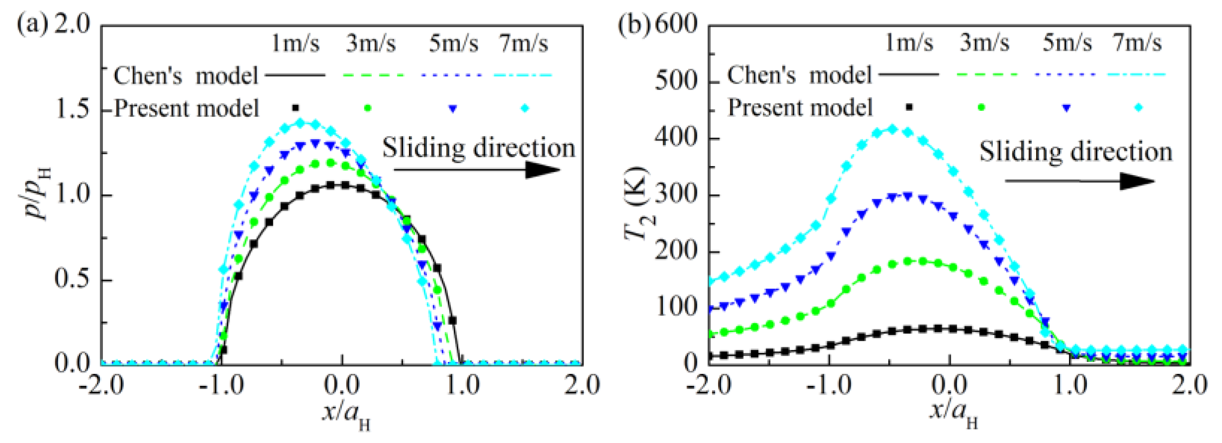
3. Verification of the Present Model

In order to validate the present model, the solutions obtained with it for the thermoelastic contact between a homogeneous solid of substrate material and an elastic ball are compared with those obtained with Chen’s model in [4]. The input parameters for the present model are shown in

Table 1. Input parameters of present model for simulating the thermoelastic contact between a homogeneous solid and an elastic ball.

Name and Unit of the Input Parameter	Value
Elasticity modulus of the ball, E (GPa)	2.1 × 102
Poisson ratio of the ball, ν	3 × 10−1
Thermal conductivity of the ball, κ (W/m·K)	5.02 × 101
Volumetric heat capacity of the ball, c (J/m3·K)	5.02 × 105
Thermal expansion coefficient of the ball, α (m/m·K)	1.17 × 10−5
Elasticity modulus of the substrate, E2 (GPa)	2.1 × 102
Poisson ratio of the substrate, ν2	3 × 10−1
Thermal conductivity of the substrate, κ2 (W/m·K)	5.02 × 101
Volumetric heat capacity of the substrate, c2 (J/m3·K)	5.02 × 105
Thermal expansion coefficient of the substrate, α2 (m/m·K)	1.17 × 10−5
Elasticity modulus of the coating, E1 (GPa)	E2
Poisson ratio of the coating, ν1	ν2
Thermal conductivity of the coating, κ1 (W/m·K)	κ2
Volumetric heat capacity of the coating, c1 (J/m3·K)	c2
Thermal expansion coefficient of the coating, α1 (m/m·K)	α2
Radius of ball, R (m)	1.0 × 10−2
External normal load, W (N)	20
Friction coefficient, μf	0.1
Sliding velocity, Vs (m/s)	0–10
Coating thickness, h (m)	aH

Note: (1) The coating has the same thermoelastic properties as those of the substrate, therefore E₁ = E₂, ν₁ = ν₂, κ₁ = κ₂, c₁ = c₂, c₁ = c₂ and α₁ = α₂ in the table; (2) The symbol a_H is the contact radius of the substrate material in Hertz point contact with the ball, which has been mentioned in Section 2.1. In this simulation, the coating thickness equals to the contact radius of the substrate material in Hertz point contact with the ball.

.

The thermoelastic properties of the coating are the same to those of the substrate when the present model is adopted to simulate the contact between a homogeneous solid of substrate material and an elastic ball. Figure 4 compares the contact pressure and the surface temperature rise along x axis under various sliding speeds, where p_H and a_H represent the maximum contact pressure and the contact radius of the substrate material in Hertz point contact. As indicated in Figure 4, the contact pressure and the surface temperature rise obtained with the present model are in an excellent match with those obtained with Chen’s model for various sliding speeds. The comparisons of the temperature rise T₂ and the von Mises stress σ_V are shown in Figure 5 and Figure 6, respectively. It can be seen that the temperature rise and the von Mises stress obtained with the present model are also in an excellent agreement with those obtained with Chen’s model for different sliding speeds.

The comparisons conducted above not only validate the present contact model, but also show that the present model can be utilized to analyze the thermoelastic contact problem of homogeneous solids.

4. Numerical Results and Discussion

In this section, the effect of the sliding speed, thermoelastic properties and thickness of the coating on the contact behavior is numerically investigated with the present model. The thermoelastic properties of the coated solid and the elastic ball and the other concerning parameters are listed in

Table 2. Thermoelastic properties of the coated solid and the elastic ball and the other concerning parameters.

Name and Unit of the Input Parameter	Value
Elasticity modulus of the ball, E (GPa)	2.1 × 102
Poisson ratio of the ball, ν	3 × 10−1
Thermal conductivity of the ball, κ (W/mK)	5.02 × 101
Volumetric heat capacity of the ball, c (J/m3·K)	5.02 × 105
Thermal expansion coefficient of the ball, α (m/mK)	1.17 × 10−5
Elasticity modulus of the substrate, E2 (GPa)	2.1 × 102
Poisson ratio of the substrate, ν2	3 × 10−1
Thermal conductivity of the substrate, κ2 (W/mK)	5.02 × 101
Volumetric heat capacity of the substrate, c2 (J/m3·K)	5.02 × 105
Thermal expansion coefficient of the substrate, α2 (m/mK)	1.17 × 10−5
Elasticity modulus of the coating, E1 (GPa)	2E2
Poisson ratio of the coating, ν1	ν2
Thermal conductivity of the coating, κ1 (W/mK)	0.5κ2–2κ2
Volumetric heat capacity of the coating, c1 (J/m3·K)	0.5c2–2c2
Thermal expansion coefficient of the coating, α1 (m/mK)	0.5α2–2α2
Radius of ball, R (m)	1.0 × 10−2
External normal load, W (N)	30
Friction coefficient, μf	0.1
Sliding velocity, Vs (m/s)	0–10
Coating thickness, h (m)	0–2aH

Note: (1) In the numerical simulation, a hard coating which has an elastic modulus equals to two times of that of substrate and a Poisson ratio equals to that of the substrate, so E₁ = 2E₂ and ν₁ = ν₂ in the table.

.

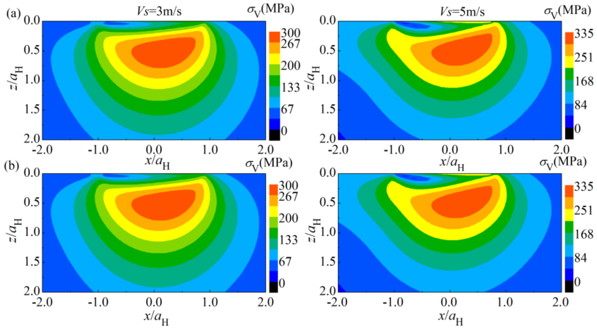
4.1. Effect of the Sliding Velocity

The sliding velocity V_s has a significant effect on the contact behavior of coated solids as shown in Figure 7. When V_s increases from 0.5 to 6 m/s, the maximum contact pressure increases to 1.8p_H from 1.2p_H and the maximum temperature rise also increases to 546 K from about 10 K. The main reason for the increase of the maximum temperature rise is that the increase of the sliding speed produces more frictional heat on the contact interface, as shown in Equation (6), which also leads to an increase of the surface thermal displacement as well as the maximum contact pressure. The heat partition coefficient H_pc also increases with the increase of the sliding speed, since more cool surfaces of the coated solid pass through the contact zone in a given time and it absorbs and takes away more frictional heat flux when passing through the contact zone. The transverse stress σ_xx at the tail side of the contact zone changes to compressive stress from tensile stress with the increase of the sliding speed as shown in Figure 7d, since the thermal stress σ_xx caused by the frictional heat flux is compressive and increases with the increase of the sliding speed. The transverse stress σ_xx at the base of the coating is tensile around the contact center and its maximum basically increases with the increase of V_s. The main reason should be the concentration of the contact pressure distribution as shown in Figure 7a. The maximum shear stress σ_zx on the interface also increases with the increase of V_s. In addition to the concentration of the contact pressure distribution, another reason is that the thermal shear stress caused by the frictional heat flux has the same direction as that caused by the surface mechanical loading at the position where the maximum σ_zx locates.

4.2. Effect of the Coating Thermal Conductivity

The effect of the coating thermal conductivity κ₁ on the contact behavior is shown in Figure 8.

When the coating thermal conductivity κ_₁ increases from 0.5κ₂ to 2κ₂, the maximum contact pressure decreases to 1.5p_H from 2.2p_H and the maximum temperature rise of the coated solid decreases to 260 K from 716 K. With the increase of κ₁, the frictional heat flux transfers more quickly into the coated solid from the contact interface, therefore the maximum temperature rise of the coated solid decreases. That is also the reason why H_pc increases with the increase of the coating thermal conductivity, as shown in Figure 8c. The surface thermal displacement decreases as a consequence of the decrease of the temperature rise caused by the increase of the coating thermal conductivity. That is the reason why the maximum contact pressure decreases with the increase of the coating thermal conductivity. The transverse stress σ_xx on the surface is compressive and its maximum decreases with the increase of κ₁, the transverse stress σ_xx at the base of the coating around the contact center is tensile and its maximum decreases with the increase of κ₁. The maximum of the shear stress σ_zx also decreases with the increase of κ₁. One reason is the deconcentration of the contact pressure distribution caused by the increase of κ₁, the other reason may be that the temperature gradient from the surface to the interface becomes relatively small with the increase of κ₁.

4.3. Effect of the Coating Volumetric Heat Capacity

The effect of the coating volumetric heat capacity c₁ on the contact behavior is shown in Figure 9. When the coating volumetric heat capacity c₁ increases from 0.5c₂ to 2c₂, the maximum contact pressure decreases from 1.9p_H to 1.59p_H and the maximum temperature rise of coated solid decreases to 375 from 519 K. The frictional heat partition coefficient increases with the increase of the coating volumetric heat capacity since a unit volume material of the coating absorbs more heat for 1 K temperature rise with the increase of the coating volumetric heat capacity. That is also the explanation for the influence of the coating volumetric heat capacity on the contact pressure and the temperature rise. Around the contact center, the maximum of the compressive stress σ_xx on the surface decreases with the increase of c₁, while the maximum tensile stress σ_xx at the base of the coating increases. The maximum of the shear stress σ_zx on the interface also decreases with the increase of c₁, as shown in Figure 9f.

4.4. Effect of the Coating Thermal Expansion Coefficient

The effect of the coating thermal expansion coefficient α₁ is shown in Figure 10. When the coating thermal expansion coefficient α₁ increases from 0.5α₂ to 2α₂, both the maximum contact pressure and the maximum temperature rise increase, as indicated in Figure 10a,b. However, its effect on the heat partition coefficient is very small, which is shown in Figure 10c. Actually, the thermal expansion coefficient itself has no effect on the heat partition coefficient H_pc, and the slight decrease of H_pc may be due to the concentration of the contact pressure, since nothing of the heat partition model has a direct relationship with the thermal expansion coefficient except that the frictional heat flux distribution is related to the contact pressure distribution. The effect of the coating thermal expansion coefficient on the contact pressure can be easily understood, since the increase of α₁ leads to an increase of the surface thermal displacement in the heated zone. With the increase of α₁, the increase of the maximum temperature rise is mainly caused by the concentration of the frictional heat flux. This result is consistent with that in [27], although the research in [27] is on a two-dimensional thermoelastic problem. The transverse stress σ_xx at the base of the coating is tensile around the contact center, however its maximum is almost the same for various α₁. This result may be explained by a mutual cancellation of the compressive thermal stress σ_xx and the tensile mechanical stress σ_xx, since not only the tensile mechanical stress σ_xx caused by the mechanical loading increases with the increase of α₁, but also the compressive thermal stress σ_xx caused by the frictional heat flux increases. The maximum shear stress σ_zx on the contact interface increases with the increase of α₁. One reason is the concentration of contact pressure caused by the increase of α₁, the other reason could be that the thermal shear stress α₁ on the interface caused by the frictional heat flux has the same direction with that caused by the mechanical loading at the position where the maximum shear stress σ_zx locates and increases with the increase of α₁.

4.5. Effect of the Coating Thickness

For various κ_1/κ₂, the effect of the coating thickness on the maximum contact pressure, the maximum temperature rise and the heat partition coefficient is show in Figure 11. Among various κ_1/κ₂, the maximum contact pressure increases fastest with the increase of coating thickness for κ_1/κ₂ = 0.5. One reason is that the coating–substrate system becomes stiffer with the increase of coating thickness since the elasticity moduli of the coating is two times of the substrate, the other reason is κ_1/κ₂ = 0.5, which leads to the maximum temperature rise increases with the increase of the coating thickness shown as Figure 11b since the frictional heat flux transfers more slowly into the coated solid with the increase of the coating thickness and less frictional heat flows into the coated solid as indicated in Figure 11c. As a result of the increase of the temperature rise, the surface thermal displacement in the contact zone increases, which will lead to the concentration of the contact pressure and the increase of the maximum contact pressure. On the contrary, the maximum temperature rise of the coated solid with κ_1/κ₂ = 2 decreases with the increase of the coating thickness as shown in Figure 11b, since the frictional heat transfers more quickly into the coated solid with the increase of the coating thickness and more frictional heat flows into the coated solid as indicated in Figure 11c. As a result of the decrease of the temperature rise, the surface thermal displacement also decreases in the contact zone of the coating–substrate system with κ_1/κ₂ = 2, therefore a low point of the maximum contact pressure is observed for κ_1/κ₂ = 2 when the coating thickness is about 0.25a_H, as shown in Figure 11a. For coated solids with κ_1/κ₂ = 1, the increase of the coating thickness leads to a concentration of the contact pressure distribution and an increase of the maximum contact pressure as indicated in Figure 11a, since the coating–substrate system becomes stiffer as a whole. As a result of the concentration of the contact pressure distribution, the maximum temperature rise increases as indicated in Figure 11b, and the heat partition coefficient decreases slightly as indicated in Figure 11c. This result is similar to the effect of the coating thermal expansion coefficient on the temperature rise and the heat partition coefficient as shown in Section 4.4. It also can be observed that the increase of the coating thickness ranging from 0 to a_H has a significant effect on the contact behavior of coated solids, however a further increase of coating thickness only brings a marginal effect on the contact behavior when the coating thickness is larger than a_H.

5. Conclusions

Based on the FRFs of coated solids subjected to the mechanical loading coupling with the heat flux on its surface, a three-dimensional thermoelastic contact model of coated solids with the frictional heat partition considered has been developed by introducing a heat partition model, and validated through a comparison of the contact pressure, temperature rise and von Mises stress in the subsurface between the present model and a model in literature. A numerical investigation of the effect of the sliding speed, thermoelastic properties and thickness of the coating on the contact behavior has been conducted by utilizing the present model. The numerical results show that the contact behavior of coated solids can be severely affected by the thermoelastic properties and thickness of the coating as well as the sliding speed. Several specific conclusions can be drawn:

• With the increase of the sliding speed, the maximum contact pressure, the maximum temperature rise, the heat partition coefficient, the maximum tensile stress of σ_xx at the base of the coating and the maximum shear stress σ_zx on the interface all increase.
• With the increase of the coating thermal conductivity, the maximum contact pressure, the maximum temperature rise, the maximum tensile stress of σ_xx at the base of the coating and maximum shear stress σ_zx on the interface decrease, the heat partition coefficient increases.
• With the increase of the coating volumetric heat capacity, the maximum contact pressure, the maximum temperature rise and the maximum shear stress σ_zx on the interface decrease, the heat partition coefficient and the maximum tensile stress of σ_xx at the base of the coating increase.
• With the increase of the coating thermal expansion coefficient, the maximum contact pressure, the maximum temperature rise and the maximum shear stress σ_zx on the interface increase, the heat partition coefficient and the maximum tensile stress of σ_xx at the base of the coating vary slightly.
• The increase of the coating thickness h ranging from 0 to a_H exerts a significant effect on the contact behavior, however a further increase of the coating thickness h only brings a marginal effect.

References

1. Kalin, M.; Vizintin, J. The tribological performance of DLC-coated gears lubricated with biodegradable oil in various pinion/gear material combinations. Wear 2005, 259, 1270–1280. [Google Scholar] [CrossRef]
2. Moorthy, V.; Shaw, B.A. Contact fatigue performance of helical gears with surface coatings. Wear 2012, 276, 130–140. [Google Scholar] [CrossRef]
3. Chen, L.; Yang, M.C.; Song, C.F.; Yu, B.J.; Qian, L.M. Is 2 nm DLC coating enough to resist the nanowear of silicon. Wear 2013, 302, 909–917. [Google Scholar] [CrossRef]
4. Chen, W.W.; Wang, Q.J. Thermomechanical analysis of elastoplastic bodies in a sliding spherical contact and the effects of sliding speed, heat partition, and thermal softening. J. Tribol. 2008, 130, 041402. [Google Scholar] [CrossRef]
5. Sneddon, I.N. Fourier Transforms; McGraw-Hill: New York, NY, USA, 1951. [Google Scholar]
6. Burmister, D.M. The general theory of stresses and displacements in layered systems. I. J. Appl. Phys. 1945, 16, 89–94. [Google Scholar] [CrossRef]
7. Burmister, D.M. The general theory of stresses and displacements in layered soil systems. III. J. Appl. Phys. 1945, 16, 296–302. [Google Scholar] [CrossRef]
8. Chen, W.T. Computation of stresses and displacements in a layered elastic medium. Int. J. Eng. Sci. 1971, 9, 775–800. [Google Scholar] [CrossRef]
9. Chen, W.T.; Engel, P.A. Impact and contact stress analysis in multilayer media. Int. J. Solids Struct. 1972, 8, 1257–1281. [Google Scholar] [CrossRef]
10. O’Sullivan, T.C.; King, R.B. Sliding contact stress-field due to a spherical indenter on a layered elastic half-space. J. Tribol. 1988, 110, 235–240. [Google Scholar] [CrossRef]
11. Nogi, T.; Kato, T. Influence of a hard surface layer on the limit of elastic contact—Part I: Analysis using a real surface model. J. Tribol. 1997, 119, 493–500. [Google Scholar] [CrossRef]
12. Cai, S.; Bhushan, B. A numerical three-dimensional contact model for rough, multilayered elastic/plastic solid surfaces. Wear 2005, 259, 1408–1423. [Google Scholar] [CrossRef]
13. Wang, Z.J.; Wang, W.Z.; Wang, H.; Zhu, D.; Hu, Y.Z. Partial slip contact analysis on three-dimensional elastic layered half space. J. Tribol. 2010, 132, 021403. [Google Scholar] [CrossRef]
14. Kot, M. Contact mechanics of coating-substrate systems: Monolayer and multilayer coatings. Arch. Civ. Mech. Eng. 2012, 12, 464–470. [Google Scholar] [CrossRef]
15. Wang, T.J.; Wang, L.Q.; Gu, L.; Zheng, D.Z. Stress analysis of elastic coated solids in point contact. Tribol. Int. 2015, 86, 52–61. [Google Scholar] [CrossRef]
16. Chen, W.W.; Zhou, K.; Keer, L.M.; Wang, Q.J. Modeling elasto-plastic indentation on layered materials using the equivalent inclusion method. Int. J. Solids Struct. 2010, 47, 2841–2854. [Google Scholar] [CrossRef]
17. Kral, E.R.; Komvopoulos, K.; Bogy, D.B. Finite element analysis of repeated indentation of an elastic-plastic layered medium by a rigid sphere, Part I: Surface results. J. Appl. Mech. 1995, 62, 20–28. [Google Scholar] [CrossRef]
18. Kral, E.R.; Komvopoulos, K. Three-dimensional finite element analysis of subsurface stress and strain fields due to sliding contact on an elastic-plastic layered medium. J. Tribol. 1997, 119, 332–341. [Google Scholar] [CrossRef]
19. Kang, J.J.; Xu, B.S.; Wang, H.D.; Wang, C.B. Competing failure mechanism and life prediction of plasma sprayed composite ceramic coating in rolling-sliding contact condition. Tribol. Int. 2014, 73, 128–137. [Google Scholar] [CrossRef]
20. Carslaw, H.; Jaeger, J.C. Conduction of Heat in Solids; Oxford University Press: London, UK, 1959. [Google Scholar]
21. Barber, J.R.; Martin-Moran, C.J. Green’s functions for transient thermoelastic contact problems for the half-plane. Wear 1982, 79, 11–19. [Google Scholar] [CrossRef]
22. Barber, J.R. Thermoelastic displacements and stresses due to a heat source moving over the surface of a half plane. J. Appl. Mech. 1984, 51, 636–640. [Google Scholar] [CrossRef]
23. Wang, Q.; Liu, G. A thermoelastic asperity contact model considering steady-state heat transfer. Tribol. Trans. 1999, 42, 763–770. [Google Scholar] [CrossRef]
24. Liu, S.; Wang, Q. A three-dimensional thermomechanical model of contact between non-conforming rough surfaces. J. Tribol. 2001, 123, 17–26. [Google Scholar] [CrossRef]
25. Leroy, J.M.; Floquet, A.; Villechaise, B. Thermomechanical behavior of multilayered media: Theory. J. Tribol. 1989, 111, 538–544. [Google Scholar] [CrossRef]
26. Leroy, J.M.; Floquet, A.; Villechaise, B. Thermomechanical behavior of multilayered media: Results. J. Tribol. 1990, 112, 317–323. [Google Scholar] [CrossRef]
27. Ju, Y.; Farris, T.N. FFT thermoelastic solutions for moving heat sources. J. Tribol. 1997, 119, 156–162. [Google Scholar] [CrossRef]
28. Shodja, H.M.; Ghahremaninejad, A. An FGM coated elastic solid under thermomechanical loading: A two dimensional linear elastic approach. Surf. Coat. Technol. 2006, 200, 4050–4064. [Google Scholar] [CrossRef]
29. Liu, J.; Ke, L.L.; Wang, Y.S. Two-dimensional thermoelastic contact problem of functionally graded materials involving frictional heating. Int. J. Solids Struct. 2011, 48, 2536–2548. [Google Scholar] [CrossRef]
30. Shi, Z. Mechanical and Thermal Contact Analysis in Layered Elastic Solids. Ph.D. Thesis, University of Minnesota, Minneapolis, MN, USA, November 2001. [Google Scholar]
31. Kulkarni, S.M.; Rubin, C.A.; Hahn, G.T. Elasto-plastic coupled temperature-displacement finite element analysis of two-dimensional rolling-sliding contact with a translating heat source. J. Tribol. 1991, 113, 93–101. [Google Scholar] [CrossRef]
32. Ye, N.; Komvopoulos, K. Three-dimensional finite element analysis of elastic-plastic layered media under thermomechanical surface loading. J. Tribol. 2003, 125, 52–59. [Google Scholar] [CrossRef]
33. Gong, Z.Q.; Komvopoulos, K. Mechanical and thermomechanical elastic-plastic contact analysis of layered media with patterned surfaces. J. Tribol. 2004, 126, 9–17. [Google Scholar] [CrossRef]
34. Guan, X.Y.; Lu, Z.B.; Wang, L.P. Achieving high tribological performance of graphite-like carbon coatings on ti6al4v in aqueous environments by gradient interface design. Tribol. Lett. 2011, 44, 315. [Google Scholar] [CrossRef]
35. Khotsyanovskii, A.O.; Kumurzhi, A.Y.; Lyashenko, B.A. Improvement of strength and wear resistance of metal products with ion-plasma nitride coatings by pulse technique implementations. Strength Mater. 2014, 46, 422–428. [Google Scholar] [CrossRef]
36. Czyzniewski, A. Optimising deposition parameters of W-DLC coatings for tool materials of high speed steel and cemented carbide. Vacuum 2012, 86, 2140–2147. [Google Scholar] [CrossRef]
37. He, D.; Li, X.; Pu, J.; Wang, L.; Zhang, G.; Liu, Z.; Li, W.; Xue, Q. Improving the mechanical and tribological properties of TiB2/a-C nanomultilayers by structural optimization. Ceram. Int. 2018, 44, 3356–3363. [Google Scholar] [CrossRef]
38. Johnson, K.L. Non-Hertzian normal contact of elastic contact bodies. In Contact Mechanics; Cambridge University Press: Cambridge, UK, 1985; pp. 107–144. [Google Scholar]
39. Polonsky, I.A.; Keer, L.M. A numerical method for solving rough contact problems based on the multi-level multi-summation and conjugate gradient techniques. Wear 1999, 231, 206–219. [Google Scholar] [CrossRef]
40. Wang, W.Z.; Hu, Y.Z.; Wang, H. Dry contact analysis based on the conjugate gradient methods and fast fourier transformation. Chin. J. Mech. Eng. 2006, 42, 14–18. (In Chinese) [Google Scholar] [CrossRef]
41. Liu, S.; Wang, Q.; Liu, G. A versatile method of discrete convolution and FFT (DC-FFT) for contact analyses. Wear 2000, 243, 101–111. [Google Scholar] [CrossRef]
42. Azarkhin, A.; Barber, J.R. Transient thermoelastic contact problem of two sliding half-planes. Wear 1985, 102, 1–13. [Google Scholar] [CrossRef] [Green Version]
43. Boucly, V.; Nélias, D.; Liu, S.; Wang, Q.J.; Keer, L.M. Contact analyses for bodies with frictional heating and plastic behavior. J. Tribol. 2005, 127, 355–364. [Google Scholar] [CrossRef]
44. Blok, H. Theoretical study of temperature rise at surfaces of actual contact under oiliness lubricating conditions. In Proceedings of the General Discussion on Lubrication and Lubricants, London, UK, 13–15 October 1937; Volume 2, pp. 222–235. [Google Scholar]
45. Tian, X.; Kennedy, F.E. Maximum and average flash temperatures in sliding contacts. J. Tribol. 1994, 116, 167–174. [Google Scholar] [CrossRef]
46. Jaegar, J.C. Moving sources of heat and the temperature at sliding surfaces. J. Proc. R. Soc. NSW 1942, 76, 202. [Google Scholar]
47. Archard, J.F.; Rowntree, R.A. The temperature of rubbing bodies; part 2, the distribution of temperatures. Wear 1988, 128, 1–17. [Google Scholar] [CrossRef]
48. Francis, H.A. Interfacial temperature distribution within a sliding hertzian contact. ASLE Trans. 1971, 14, 41–54. [Google Scholar] [CrossRef]
49. Gao, J.; Lee, S.C.; Ai, X.; Nixon, H. An FFT-based transient flash temperature model for general three-dimensional rough surface contacts. J. Tribol. 2000, 122, 519–523. [Google Scholar] [CrossRef]
50. Bos, J.; Moes, H. Frictional heating of tribological contacts. J. Tribol. 1995, 117, 171–177. [Google Scholar] [CrossRef]
51. Shewchuk, J.R. An Introduction to the Conjugate Gradient Method without the Agonizing Pain; Carnegie Mellon University: Pittsburgh, PA, USA, 1994. [Google Scholar]
52. Ahmadi, N.L.M.T.; Keer, L.M.; Mura, T. Non-Hertzian contact stress analysis for an elastic half-space normal and sliding contact. Int. J. Solids Struct. 1983, 19, 357–373. [Google Scholar] [CrossRef]
53. Ju, Y.; Farris, T.N. Spectral analysis of two-dimensional contact problems. J. Tribol. 1996, 118, 320–328. [Google Scholar] [CrossRef]
54. Liu, S.; Wang, Q. Studying contact stress fields caused by surface tractions with a discrete convolution and fast fourier transform algorithm. J. Tribol. 2002, 124, 36–45. [Google Scholar] [CrossRef]
55. Kul’chyts’kyi-Zhyhailo, R.; Bajkowski, A. Elastic coating with inhomogeneous interlayer under the action of normal and tangential forces. Mater. Sci. 2014, 49, 650–659. [Google Scholar] [CrossRef]
Figure 1. Description of the thermoelastic contact between an elastic ball and a half space coated with a homogeneous coating considering the frictional heat partition.
Coatings 08 00470 g001
Figure 2. The algorithm flow chart: (a) overall flow chart of the thermal elastic contact model, (b) flow chart of the heat partition model.
Coatings 08 00470 g002
Figure 3. Half space coated with a homogeneous coating subjected to the coupled action of the mechanical loading and the frictional heat flux.
Coatings 08 00470 g003
Figure 4. Comparisons on the contact pressure and the surface temperature rise between the present model and Chen’s model under various sliding speeds: (a) contact pressure along x axis, (b) surface temperature rise along x axis.
Coatings 08 00470 g004
Figure 5. Comparison on the temperature rise in xoz plane between the present model and Chen’s model under different sliding speeds: (a) solution of Chen’s model, (b) solution of the present model.
Coatings 08 00470 g005
Figure 6. Comparison on the von Mises stress in xoz plane between the present model and Chen’s model under different sliding speeds: (a) solution of Chen’s model, (b) solution of the present model.
Coatings 08 00470 g006
Figure 7. Effect of the sliding speed Vs on: (a) contact pressure along x axis, (b) surface temperature rise along x axis, (c) frictional heat partition coefficient, (d) σxx on the surface, (e) σxx at the base of the coating, (f) σzx on the interface.
Coatings 08 00470 g007
Figure 8. Effect of the coating thermal conductivity κ1 on: (a) contact pressure along x axis, (b) surface temperature rise along x axis, (c) frictional heat partition coefficient, (d) σxx on the surface, (e) σxx at the base of the coating, (f) σzx on the interface.
Coatings 08 00470 g008
Figure 9. Effect of the coating volumetric heat capacity c1 on: (a) contact pressure along x axis, (b) surface temperature rise along x axis, (c) frictional heat partition coefficient, (d) σxx on the surface, (e) σxx at the base of the coating, (f) σzx on the interface.
Coatings 08 00470 g009
Figure 10. Effect of the coating thermal expansion coefficient α1 on: (a) contact pressure along x axis, (b) surface temperature rise along x axis, (c) frictional heat partition coefficient, (d) σxx on the surface, (e) σxx at the base of the coating, (f) σzx on the interface.
Coatings 08 00470 g010
Figure 11. Effect of the coating thickness h on: (a) maximum contact pressure, (b) maximum surface temperature, (c) frictional heat partition coefficient.
Coatings 08 00470 g011