Modeling Enthalpy of Formation with Machine Learning for Structural Evaluation and Thermodynamic Stability of Organic Semiconductors

Abstract

The enthalpy of formation (dH_m) is a crucial parameter in evaluating the structural stability of organic semiconductors. In this study, we employed machine learning (ML) models to predict the dH_m of organic semiconductors. The current results show that Kappa2 and NumRotableBonds are highly correlated with the dH_m, indicating their importance in determining the stability of these materials. Using Gradient Boosting, Random Forest, and Extra Trees models, we achieved a high R² value of 0.68–0.70, demonstrating the effectiveness of these models in predicting the dH_m. Further analysis using SHAP values revealed that Kappa2 and fr_uncrch_alkane are the most important descriptors in determining the dH_m. These findings provide valuable insights into the structural evaluation and stability of organic semiconductors and highlight the potential of ML models in predicting key properties of these materials.

1. Introduction

Organic semiconductors have gained significant attention in recent years for their potential applications in light harvesting, owing to their unique combination of properties [1]. Their importance in this context lies in their ability to efficiently absorb light and convert it into electrical energy, thereby facilitating the development of highly efficient solar cells and photovoltaic devices [2]. They also exhibit superior flexibility, low cost, and facile processability [3], which enables the fabrication of large area, flexible, and lightweight photovoltaic devices that can be easily integrated into a variety of applications [4]. The molecular structure of organic semiconductors can be tailored to optimize their optical and electrical properties [5], allowing for the design of materials with specific absorption spectra and charge transport characteristics [6]. Additionally, the use of organic semiconductors in light harvesting applications offers the potential for the development of novel device architectures, such as tandem solar cells and photodetectors [7], which can further enhance the efficiency and versatility of these devices [8]. As a result, organic semiconductors are poised to play a pivotal role in the development of next-generation light harvesting technologies [9], enabling the creation of innovative, high-performance devices that can efficiently capture and convert sunlight into usable energy [10].

The thermal properties of organic semiconductors are of paramount importance in determining their suitability for various applications, particularly in the design of thin films and devices that operate under diverse thermal conditions [11]. One crucial aspect of their thermal properties is the dH_m, which is a measure of the energy released or absorbed during the formation of a material from its constituent elements [12]. Organic semiconductors typically exhibit relatively low enthalpies of formation, which facilitates their deposition and crystallization into thin films with minimal thermal damage or degradation [13]. This property enables the design and fabrication of thin films with precise control over their morphology, crystal structure, and intermolecular interactions, which is essential for optimizing their electronic and optoelectronic properties [14]. In addition, the stability-driven features of materials, which may be characterized by their glass transition temperature, melting point, and thermal decomposition temperature, are critical in determining their reliability and durability under various operating conditions [15]. By carefully tailoring the molecular structure and processing conditions, it is possible to design organic semiconductors with optimized thermal properties [16], allowing for the fabrication of thin films and devices that can withstand elevated temperatures, thermal stress, and other environmental factors [17]. The use of high-enthalpy of formation materials can also enable the creation of thin films with enhanced thermal stability, while low-enthalpy of formation materials may be more suitable for applications requiring low-temperature processing or flexible substrates.

The integration of ML techniques has revolutionized the field of materials science, particularly in predicting relevant properties of organic semiconductors [18]. The ability to accurately predict properties such as dH_m, thermal stability [19], and electronic conductivity is crucial for the design and development of high-performance devices [20]. Its different algorithms can be trained on large datasets of experimental and computational results to identify complex relationships between the molecular structure and material properties, enabling the prediction of these properties with high accuracy [21]. This is particularly significant in the context of organic semiconductors, where the intricate relationships between molecular structure, crystal packing, and material properties make experimental characterization and traditional computational modeling approaches challenging [22]. The aim of this work is to utilize ML techniques to predict the dH_m of organic semiconductors, with a specific focus on understanding the structural basis of this property. By analyzing the relationships between molecular features, such as functional groups, molecular topology, and crystal structure, and the corresponding dH_m values, it is possible to gain insights into the underlying factors that influence this property. The predicted dH_m values can then be used to design and optimize organic semiconductors with tailored thermal properties, which is essential for the development of high-performance devices that can operate efficiently and reliably under various conditions. The structural basis of the dH_m can provide valuable information on the molecular design principles and processing conditions required to achieve optimal material properties, ultimately facilitating the discovery of new organic semiconductors with improved performance and stability. By leveraging ML techniques, this work aims to establish a robust framework for the prediction and understanding of dH_m in organic semiconductors, which can be extended to other material properties and applications, thereby accelerating the development of novel materials and devices (Figure 1). Our work presents a significant contribution to the field of organic electronics by introducing a machine learning-based approach for predicting the dH_m and evaluating the structural and thermodynamic stability of organic semiconductors, enabling the accelerated discovery of stable and efficient materials.

2. Methodology

2.1. ML Analysis

For relevant ML calculations, the latest Python program (V 3.10.14) and its latest libraries were imported. For this, all the dataset files were imported by their Pandas module [23], while the NumPy [24] and RDKit [25] libraries were imported for their descriptor designing. Their calculated results were visualized by its Matplotlib library (V3.10.3), while their scientific/statistical calculations were performed by the Scikit-learn module [26]. Their relevant plots and graphs were plotted by importing the Matplotlib library. Their molecular descriptors from their experimental results with their SMILES length (Figure 2) were designed by importing the RDKit toolkit [27]. Their descriptors were designed to realize their impact on their target property (d_Hm). An example of a few prominent descriptor relations is given below as Equations (1)–(4):

$$\mathrm{M}\mathrm{W}={\displaystyle \sum }_{\mathrm{i}=1}^{\mathrm{n}}{\mathrm{m}}_{\mathrm{i}}$$

(1)

$$\mathrm{L}\mathrm{o}\mathrm{g}\mathrm{P}={\mathrm{L}\mathrm{o}\mathrm{g}}_{10}\left({\displaystyle \frac{{\mathrm{C}}_{\mathrm{o}\mathrm{c}\mathrm{t}\mathrm{a}\mathrm{n}\mathrm{o}\mathrm{l}}}{{\mathrm{C}}_{\mathrm{w}\mathrm{a}\mathrm{t}\mathrm{e}\mathrm{r}}}}\right)$$

(2)

$$\mathrm{W}={{\displaystyle \sum }}_{\mathrm{i}=1}^{\mathrm{n}}{{\displaystyle \sum }}_{\mathrm{j}=1}^{\mathrm{n}}{\mathrm{d}}_{\mathrm{i}\mathrm{j}}$$

(3)

$$\mathrm{E}\mathrm{N}={\displaystyle \frac{1}{\mathrm{n}}}{\displaystyle \sum }_{\mathrm{i}=1}^{\mathrm{n}}{\mathrm{x}}_{\mathrm{i}}$$

(4)

To evaluate their different molecular connectivity descriptors (${\mathsf{\chi }}_{\mathrm{n}}^{\mathrm{v}}$), their hydrogen-suppressed skeletons were employed. Their valence connectivity index (${\mathsf{\chi }}_{\mathrm{o}}^{\mathrm{v}}$) [28] was designed from their non-hydrogen atoms having distinct δ^v values, as denoted by their atomic valence delta (δ^v) [29] (Equation (5)).

$${\mathsf{\chi }}_{\mathrm{o}}^{\mathrm{v}}={\sum }_{\mathrm{i}=10}^{\mathrm{n}}{\left({\delta }^{\mathrm{v}}\right)}^{-0.6}$$

(5)

Each of their non-hydrogen atoms with their atomic number (Z) and valence electrons (Z^v), along with their attached hydrogen atoms (h), calculated their δ^v after combining them (Equation (6)).

$$\delta ={\displaystyle \frac{{\mathrm{Z}}^{\mathrm{h}}-\mathrm{h}}{\mathrm{Z}-{\mathrm{Z}}^{\mathrm{h}}-1}}$$

(6)

2.2. Correlations and Feature Scores

The Pearson correlation of the target property with its designed descriptors as their coefficient (r) [30] was quantified through their linear relationship by taking their two variables, such as XX and YY (Equation (7)).

$$\mathrm{r}={\displaystyle \frac{\mathrm{n}\left(\sum \mathrm{X}\mathrm{Y}\right)-\left(\sum \mathrm{X}\right)\left(\sum \mathrm{Y}\right)}{\sqrt{\left[\mathrm{n}\sum {\mathrm{X}}^2-{\left(\sum \mathrm{X}\right)}^2\right]}\sqrt{\left[\mathrm{n}\sum {\mathrm{Y}}^2-{\left(\sum \mathrm{Y}\right)}^2\right]}}}$$

(7)

while n denoted their data point numbers, where ∑XY was the sum of the product of their paired scores (Equation (8)). Also, their feature importance scores (FI_j) for a feature j were also calculated by their evaluated models [31].

$${\mathrm{F}\mathrm{I}}_{\mathrm{j}}={\displaystyle \frac{1}{\mathrm{T}}}{{\displaystyle \sum }}_{\mathrm{t}=1}^{\mathrm{T}}{\Delta \mathrm{I}}_{\mathrm{j}\mathrm{t}}$$

(8)

where T is the total number of trees in the model, while ΔI_jt shows their decrease in their impurity of a tree (t). A tree-based model can be evaluated for its decrease in impurity, like Gini impurity or entropy [32], by bringing each feature of t.

3. Results and Discussion

3.1. Descriptor Designing

The dH_m, a measure of the energy change associated with the formation of a compound from its constituent elements, has been found to have significant correlations with several molecular descriptors. The highest correlation is with kappa2 [33], a topological index that characterizes the shape of a molecule, with a correlation coefficient of 0.66 (Figure 2). This suggests that the shape of a molecule plays a crucial role in determining its dH_m. The polymers with more complex shapes, as indicated by higher kappa2 values, tend to have higher enthalpies of formation, possibly due to the increased energy required to form and stabilize these structures. Another molecular descriptor that showed a strong correlation with dH_m is NumRotatbleBonds, which represents the number of rotatable bonds in a molecule, with a correlation coefficient of 0.62. This indicated that molecules with more rotatable bonds tend to have higher enthalpies of formation.

This could be rationalized by considering the fact that rotatable bonds introduce greater flexibility and conformational complexity to a molecule, which can lead to increased energy requirements for its formation. Furthermore, the correlation with fr_unbrch_alkane, which represents the fraction of unbranched alkane-like structures in a molecule, with a coefficient of 0.60 suggested that molecules with more linear, unbranched structures tend to have lower enthalpies of formation. The correlation with kappa1, another topological index, with a coefficient of 0.59 further reinforces the idea that molecular shape and topology play important roles in determining the dH_m. Additionally, the correlations with Chi1n and Chi1v, which were valence and non-valence connectivity indices, respectively, with coefficients around 0.56 suggested that the distribution of electrons and the overall connectivity of a molecule also influence its dH_m. Similarly, the correlation with NumValenceElectrons, which represents the total number of valence electrons in a molecule, with a coefficient of 0.56 indicated that the electron density and valence electron configuration of a molecule contribute to its dH_m. All these correlations suggest that the dH_m is a complex property that is influenced by a combination of molecular shape, topology, flexibility, and electronic structure.

3.2. Model Evaluation

The evaluation of ensemble and non-ensemble ML models to estimate their performance against experimental d_Hm values is a comprehensive process that involves assessing the predictive capabilities of various algorithms. Among the models evaluated, Gradient Boosting (GB) [34], Random Forest (RF) [35], Extra Trees [36], and Historical Gradient Boosting (Hist GB) [37] were notable for their ability to accurately predict d_Hm values. The GB is a powerful ensemble learning regressor that combines multiple weak models to create a strong predictive model, working by iteratively training decision trees, with each subsequent tree attempting to correct the errors of the previous one (Figure 3). RF and Extra Trees are also ensemble methods that are based on the concept of decision trees, with RF combining multiple trees to improve accuracy and robustness and Extra Trees using a technique called “averaging” to combine the predictions of individual trees. The Hist GB, on the other hand, incorporates temporal information into the model, allowing it to capture patterns and trends in the data over time. The evaluation of these models against experimental d_Hm values involves comparing their predicted values to the actual values obtained from experiments, using metrics such as mean absolute error, mean squared error, and coefficient of determination.

The performance of the four best regression models, namely GB, RF, Extra Trees, and Hist GB, can be evaluated based on their R² and RMSE values. The R² value, also known as the coefficient of determination, measures the proportion of the variance in the dependent variable that is predictable from the independent variable(s). The RMSE value, on the other hand, measures the average magnitude of the errors in the model’s predictions. Among the four models, RF has the highest R² value of 0.70, indicating that it is able to explain 70% of the variance in the dependent variable. This suggested that RF was the most effective model in terms of capturing the underlying patterns and relationships in the data.

In terms of RMSE, RF also has the lowest value of 11.27, indicating that its predictions were, on average, closest to the actual values. This could be a significant finding, as it suggested that RF was not only able to capture the underlying patterns in the data but could also be able to make accurate predictions (Figure 4). The Extra Trees and Hist GB regressors had their identical R² and RMSE values of 0.69 and 11.50, respectively, suggesting that they could be equally effective in terms of explaining the variance in the dependent variable and making accurate predictions. GB, on the other hand, has the lowest R² value of 0.68 and the highest RMSE value of 11.68, indicating that it could be the least effective model among the four.

The performance of these models can be attributed to their respective strengths and weaknesses. The RF regressor, for example, is known for its ability to handle high-dimensional data and to reduce overfitting, which might explain its strong performance in this case. The Extra Trees and Hist GB regressors, on the other hand, are both ensemble methods that combine multiple models to improve their predictive performance, which might explain their similar performance. The GB regressor, while a powerful algorithm, might be more prone to overfitting, which may explain its relatively poor performance.

The implications of these findings could be significant in suggesting that RF might be the most suitable model for predicting d_Hm values in this particular context [38]. This is because RF is able to capture the underlying patterns and relationships in the data and make accurate predictions, which is critical in many applications. Furthermore, the fact that Extra Trees and Hist GB have similar performance to RF suggests that they might also be suitable alternatives, particularly if there are specific requirements or constraints that need to be considered [39]. In contrast, the GB regressor might require further tuning or modification to improve its performance, which might involve adjusting its hyperparameters or using techniques such as regularization to reduce overfitting. The results of this analysis could have important implications for the development of predictive models for d_Hm values and highlight the importance of carefully evaluating and comparing the performance of different models.

The density of residuals for each of the four models provides valuable insights into their performance and behavior [40]. The residuals, which represented the differences between the actual and predicted d_Hm values, were spread out across a range of values, indicating that each model could be capable of capturing a significant portion of the variability in the data. However, the specific characteristics of the residual distributions vary across the models. For example, GB and RF had similar residual ranges, spanning from −40 to 100, and predicted d_Hm values ranging from 0 to 175 (Figure 5). This suggested that those two models could be capable of handling a similar range of values and that their predictions could be centered around a similar range. In contrast, Extra Trees and Hist GB had slightly different residual characteristics. Extra Trees had a broader residual range, spanning from −60 to 100, and predicted d_Hm values ranging from 0 to 200. That indicated that Extra Trees was capable of handling a wider range of values and that its predictions were more spread out. The Hist GB, on the other hand, had a similar residual range to Extra Trees, spanning from −60 to 100, but its predicted d_Hm values are more limited, ranging from 0 to 150. This suggested that Hist GB was capable of handling a similar range of values to Extra Trees, but its predictions were more conservative.

3.3. SHapley Impact

The SHAP value beeswarm plot of the evaluated model reveals valuable insights into the relative importance of each descriptor in predicting the d_Hm values. According to the plot, kappa2 emerged as the descriptor with the highest impact, indicating that it was the most influential feature in determining its model predictions. This is not surprising, given that kappa2 is a molecular descriptor that captures the spatial arrangement of atoms within a molecule, which can have a significant impact on its thermodynamic properties [41], including the heat of melting (Figure 6). The fact that kappa2 is the most important descriptor suggested that the model could be heavily reliant on the spatial arrangement of atoms in the molecule to make predictions. The next most important descriptor, fr_unbrch_alkane, was a functional group count descriptor that represents the number of unbranched alkane groups in the molecule. The presence of this descriptor in the top two suggested that the model was also considering the molecular structure and functional groups present in the molecule when making predictions. The fact that fr_unbrch_alkane followed kappa2 in importance indicated that the model was using a combination of spatial arrangement and functional group information to predict the d_Hm values. The third most important descriptor, kappa1, was another molecular descriptor that captures the spatial arrangement of atoms but with a slightly different focus than kappa2. The presence of kappa1 in the top three suggested that the model was using multiple molecular descriptors to capture different aspects of the molecular structure.

The remaining descriptors in the top list, including kappa3, TPSA, VSA_Estate8, and Chi1, also provided valuable insights into the model behavior. Kappa3 was another molecular descriptor that captured the spatial arrangement of atoms but with a focus on their molecular shape and size. TPSA, or topological polar surface area, was a descriptor that represented the surface area of the molecule that was accessible to a solvent. VSA_Estate8 was a descriptor that represented the van der Waals surface area of the molecule, while Chi1 was a descriptor that captured the molecular connectivity. The presence of these descriptors in the top list suggested that the model was using a combination of molecular structure, functional group, and surface area information to predict d_Hm values. Overall, the SHAP values beeswarm plot provided a detailed understanding of the model behavior and the relative importance of each descriptor in predicting d_Hm values.

3.4. Cross Validation

The K-fold cross-validation analysis for the model reveals a comprehensive evaluation of its performance across different folds [42]. The analysis was conducted for zero to four folds (five folds), where the data were divided into five folds and the model was trained and tested on each fold separately. Their training R² values ranged from 0.72 to 0.77, indicating that the model was able to capture the underlying patterns in the data and fit the training data well. The test R² values, which were a more reliable indicator of the model performance, ranged from 0.55 to 0.67. While the test R² values were lower than the training R² values, they were still relatively high, indicating that the model could be able to generalize well to unseen data (Figure 7). The fact that the test R² values were consistent across the different folds suggested that the model was robust and not sensitive to the specific data used for training and testing. The highest test R² value of 0.67 was observed in fold four, which suggested that the model might be overfitting to the training data in this fold. However, the difference between the training and test R² values was not significant enough to indicate severe overfitting. The K-fold cross-validation analysis also provided insight into the model performance across different folds. Fold one had the lowest test R² value of 0.55, which might indicate that the model was struggling to generalize to this particular set of data (Figure 7). In contrast, fold four had the highest test R² value of 0.67, which suggested that the model was performing well on this set of data. The fact that the model performance varied across the different folds might indicate that the data were not perfectly representative of the underlying population or that the model was sensitive to certain characteristics of the data. The K-fold cross-validation analysis suggested that the model was performing well, with high R² values for both training and testing sets. The consistency of the test R² values across the different folds indicated that the model could be robust and able to generalize well to unseen data. However, the variation in the model performance across the different folds might indicate that further refinement of the model could be necessary to improve its performance and robustness. Additionally, the analysis highlighted the importance of using K-fold cross-validation to evaluate the model performance, as it provided a more comprehensive understanding of the model strengths and weaknesses than a single train–test split.

3.5. Hyperparameter Tuning

The hyperparameter tuning of the model revealed a comprehensive analysis of the learning rate impact on its performance [43]. The results showed that the model test score was highly sensitive to the learning rate, with a significant range of values resulting in varying degrees of performance. For learning rates between −25 and 1.25, the test score ranged up to 0.7, indicating that the model was capable of achieving high accuracy when the learning rate was optimized (Figure 8).

The most notable finding was that a learning rate of up to 0.50 resulted in a test score of 0.7, which suggested that the model was able to learn effectively and generalize well to unseen data when the learning rate was moderate. This is a significant result, as it indicates that the model is robust and can achieve high performance even when the learning rate is not extremely high (Figure 8). The fact that the test score remains high for learning rates up to 0.50 suggested that the model could be able to adapt to a range of learning rates and find the optimal solution. However, for learning rates 0.05–0.80, the mean test score ranged from 0.62, indicating that the model performance was not as consistent across that range. This also suggested that the model might be overfitting or underfitting for certain learning rates, resulting in suboptimal performance.

The fact that the mean test score was lower than the maximum test score achieved at a learning rate of 0.50 suggested that the model performance was highly dependent on the learning rate and that finding the optimal learning rate was important to achieve their accuracy. For learning rates of 0.55–1.25, the test score dropped to 0.53, indicating that the model performance was negatively impacted by higher learning rates. This suggested that the model could be sensitive to overfitting when the learning rate was too high, resulting in poor generalization to unseen data. The fact that the test score dropped off significantly for learning rates above 0.55 suggested that the model performance was highly dependent on the learning rate and that finding the optimal learning rate was crucial for achieving high accuracy. The maximum depth of the model varied up to 10, with notable test scores at different depths. The maximum test score of 0.62 was achieved at a depth of 3, indicating that the model was able to capture relevant features at this depth. A higher test score of 0.67 was achieved at a depth of 5, suggesting that the model was able to learn more complex patterns at this depth. However, the mean test score at a depth of 10 was 0.65, which was slightly lower than the maximum test score at a depth of 5, indicating that increasing the depth beyond 5 may not necessarily lead to better performance.

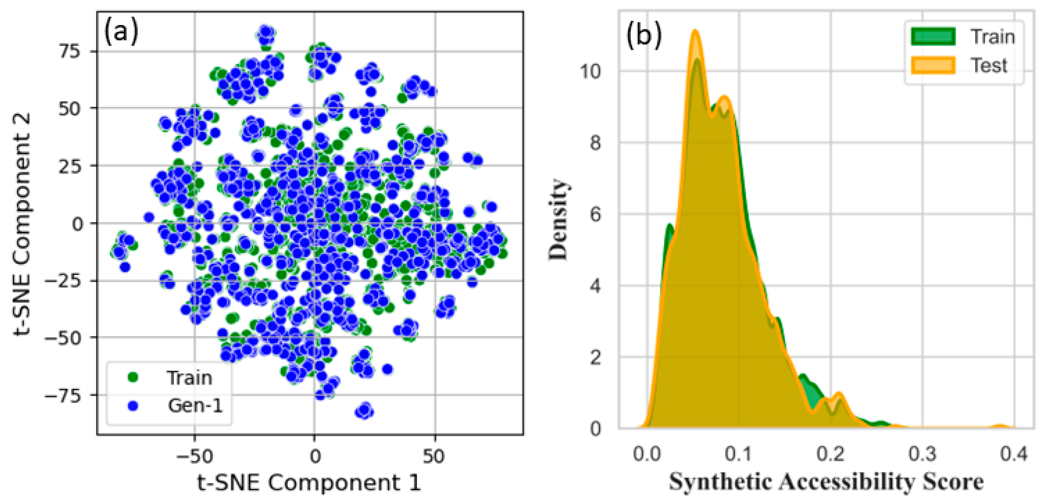
3.6. Data Clustering

The data clustering pattern of the data, in the form of its T-distributed Stochastic Neighbor Embedding (t-SNE) [44], revealed a complex and interesting structure, with two components ranging from −50 to 50 and −75 to 75, respectively. This showed that the data were not randomly distributed but rather formed clusters or groups that were separated by certain characteristics. Component 1 appeared to be the primary driver of the clustering pattern (Figure 9). The data points that fell within that range were densely packed, forming a large cluster in the center of the plot. This cluster was flanked by two smaller clusters, one on either side, which were separated from the central cluster by a gap/void in the data. The presence of those smaller clusters suggested that there might be sub-populations within the data that were distinct from the main cluster. Component 2 appeared to be secondary to component 1 in terms of its influence on the clustering pattern. However, it was still an important factor, as it could help to separate the data points into distinct groups or clusters. The data points that fell within the lower range of component 2 appeared to form a separate cluster that was distinct from the main cluster.

Similarly, the data points that fell within the upper range of component 2 also appeared to form a separate cluster. The combination of these two components resulted in a clustering pattern that was complex and multifaceted. The data points were not randomly distributed but rather formed a series of clusters and sub-clusters that were separated by gaps/voids in the data. That suggested that the data could not simply be a collection of random points but rather a structured dataset that contained hidden patterns and relationships. One possible interpretation of this clustering pattern could be that it reflected the presence of different sub-populations or groups within the data. For example, in a dataset of materials, the clusters might represent different types of materials, such as metals, polymers, or ceramics. The gaps/voids in the data might represent the boundaries between these different groups or the lack of data points in certain regions of the plot. Another possible interpretation could be that the clustering pattern reflected the presence of different characteristics or features within the data. For example, in a dataset of materials, the clusters might represent different properties or characteristics, such as strength, conductivity, or optical properties. The gaps or voids in the data might represent the absence of certain characteristics or features in certain regions of the plot.

4. Conclusions

This study demonstrated the potential of ML models in predicting the dH_m of organic semiconductors. The results showed that Kappa2 and NumRotableBonds were key descriptors that correlated with the dH_m and that the Gradient Boosting, Random Forest, and Extra Trees models achieved high predictive accuracy. The identification of fr_uncrch_alkane as an important descriptor highlighted the significance of alkane-like fragments in determining the stability of organic semiconductors. These findings had significant implications for the design and development of new organic semiconductor materials with improved stability and performance. The use of ML models to predict the dH_m of organic semiconductors accelerated the discovery of new materials and reduced the need for experimental synthesis and characterization. This approach was integrated with high-throughput computational screening and experimental validation to identify novel organic semiconductors with tailored properties. The development of more accurate and interpretable ML models provided deeper insights into the relationships between a molecular structure and material properties, enabling the design of organic semiconductors with improved efficiency, stability, and sustainability. Further studies also explored the application of ML models to predict other key properties of organic semiconductors, such as charge carrier mobility and optical absorption, to further accelerate the development of these materials for a wide range of applications, including solar cells, light-emitting diodes, and field-effect transistors.

References

1. Gopalakrishnan, V.; Balaji, D.; Dangate, M.S. Conjugated Polymer Photovoltaic Materials: Performance and Applications of Organic Semiconductors in Photovoltaics. ECS J. Solid State Sci. Technol. 2022, 11, 35001. [Google Scholar] [CrossRef]
2. Güleryüz, C.; Sumrra, S.H.; Hassan, A.U.; Mohyuddin, A.; Waheeb, A.S.; Awad, M.A.; Jalfan, A.R.; Noreen, S.; Kyhoiesh, H.A.K.; El Azab, I.H. A machine learning and DFT assisted analysis of benzodithiophene based organic dyes for possible photovoltaic applications. J. Photochem. Photobiol. A Chem. 2025, 460, 116157. [Google Scholar] [CrossRef]
3. Wu, T.; Tan, L.; Feng, Y.; Zheng, L.; Li, Y.; Sun, S.; Liu, S.; Cao, J.; Yu, Z. Toward Ultrathin: Advances in Solution-Processed Organic Semiconductor Transistors. ACS Appl. Mater. Interfaces 2024, 16, 61530–61550. [Google Scholar] [CrossRef]
4. Jia, Y.; Chen, G.; Zhao, L. Defect detection of photovoltaic modules based on improved VarifocalNet. Sci. Rep. 2024, 14, 15170. [Google Scholar] [CrossRef]
5. Dong, J.; Yan, C.; Chen, Y.; Zhou, W.; Peng, Y.; Zhang, Y.; Wang, L.-N.; Huang, Z.-H. Organic semiconductor nanostructures: Optoelectronic properties, modification strategies, and photocatalytic applications. J. Mater. Sci. Technol. 2022, 113, 175–198. [Google Scholar] [CrossRef]
6. Salzmann, I.; Heimel, G.; Oehzelt, M.; Winkler, S.; Koch, N. Molecular Electrical Doping of Organic Semiconductors: Fundamental Mechanisms and Emerging Dopant Design Rules. Acc. Chem. Res. 2016, 49, 370–378. [Google Scholar] [CrossRef] [PubMed]
7. Joly, D.; Delgado, J.L.; Atienza, C.; Martín, N. Light-Harvesting Materials for Organic Electronics. In Photonics, Volume 2: Nanophotonic Structures and Materials; Wiley: Hoboken, NJ, USA, 2015; pp. 311–341. ISBN 978-1-119-01401-0. [Google Scholar]
8. Weis, M. Organic Semiconducting Polymers in Photonic Devices: From Fundamental Properties to Emerging Applications. Appl. Sci. 2025, 15, 4028. [Google Scholar] [CrossRef]
9. Güleryüz, C.; Hassan, A.U.; Güleryüz, H.; Kyhoiesh, H.A.K.; Mahmoud, M.H.H. A machine learning assisted designing and chemical space generation of benzophenone based organic semiconductors with low lying LUMO energies. Mater. Sci. Eng. B 2025, 317, 118212. [Google Scholar] [CrossRef]
10. Kunkel, C.; Margraf, J.T.; Chen, K.; Oberhofer, H.; Reuter, K. Active discovery of organic semiconductors. Nat. Commun. 2021, 12, 2422. [Google Scholar] [CrossRef]
11. Wang, X.; Wang, W.; Yang, C.; Han, D.; Fan, H.; Zhang, J. Thermal transport in organic semiconductors. J. Appl. Phys. 2021, 130, 170902. [Google Scholar] [CrossRef]
12. Wang, X.; Peng, B.; Chan, P. Thermal Annealing Effect on the Thermal and Electrical Properties of Organic Semiconductor Thin Films. MRS Adv. 2016, 1, 1637–1643. [Google Scholar] [CrossRef]
13. Tong, W.; Li, H.; Liu, D.; Wu, Y.; Xu, M.; Wang, K. Study on the changes in the reverse recovery characteristics of high-power thyristor under 14.1 MeV fusion neutron irradiation. Fusion Eng. Des. 2025, 211, 114744. [Google Scholar] [CrossRef]
14. Miao, Z.; Gao, C.; Shen, M.; Wang, P.; Gao, H.; Wei, J.; Deng, J.; Liu, D.; Qin, Z.; Wang, P.; et al. Organic light-emitting transistors with high efficiency and narrow emission originating from intrinsic multiple-order microcavities. Nat. Mater. 2025, 24, 917–924. [Google Scholar] [CrossRef]
15. Güleryüz, C.; Sumrra, S.H.; Hassan, A.U.; Mohyuddin, A.; Elnaggar, A.Y.; Noreen, S. A machine learning analysis to predict the stability driven structural correlations of selenium-based compounds as surface enhanced materials. Mater. Chem. Phys. 2025, 339, 130786. [Google Scholar] [CrossRef]
16. Bronstein, H.; Nielsen, C.B.; Schroeder, B.C.; McCulloch, I. The role of chemical design in the performance of organic semiconductors. Nat. Rev. Chem. 2020, 4, 66–77. [Google Scholar] [CrossRef] [PubMed]
17. Wu, W.; Chen, Y.; Xie, B.; Wu, H.; Cheng, L.; Guo, Y.; Cai, C.; Chen, X. Microdynamic behaviors of Au/Ni-assisted chemical etching in fabricating silicon nanostructures. App. Surf. Sci. 2025, 696, 122915. [Google Scholar] [CrossRef]
18. Gao, S.; Wang, H.; Huang, H.; Dong, Z.; Kang, R. Predictive models for the surface roughness and subsurface damage depth of semiconductor materials in precision grinding. IJEM 2025, 7, 035103. [Google Scholar] [CrossRef]
19. Tian, X.; Xun, R.; Chang, T.; Yu, J. Distribution function of thermal ripples in h-BN, graphene and MoS2. Phys. Lett. A 2025, 550, 130597. [Google Scholar] [CrossRef]
20. Wang, H.; Hou, Y.; He, Y.; Wen, C.; Giron-Palomares, B.; Duan, Y.; Gao, B.; Vavilov, V.P.; Wang, Y. A Physical-Constrained Decomposition Method of Infrared Thermography: Pseudo Restored Heat Flux Approach Based on Ensemble Bayesian Variance Tensor Fraction. IEEE Trans. Ind. Inform. 2023, 20, 3413–3424. Available online: https://ieeexplore.ieee.org/document/10242241 (accessed on 14 June 2025). [CrossRef]
21. Armeli, G.; Peters, J.-H.; Koop, T. Machine-Learning-Based Prediction of the Glass Transition Temperature of Organic Compounds Using Experimental Data. ACS Omega 2023, 8, 12298–12309. [Google Scholar] [CrossRef]
22. Qin, X.; Wang, Q.; Zhao, X.; Xia, S.; Wang, L.; Zhang, Y.; He, C.; Chen, D.; Jiang, B. PCS: Property-composition-structure chain in Mg-Nd alloys through integrating sigmoid fitting and conditional generative adversarial network modeling. Scr. Mater. 2025, 265, 116762. [Google Scholar] [CrossRef]
23. Mckinney, W. Pandas: A Foundational Python Library for Data Analysis and Statistics. Python High Perform. Sci. Comput. 2011, 14, 1–9. [Google Scholar]
24. Schäfer, C. Extensions for Scientists: NumPy, SciPy, Matplotlib, Pandas. In Quickstart Python: An Introduction to Programming for STEM Students; Schäfer, C., Ed.; Springer Fachmedien: Wiesbaden, Germany, 2021; pp. 45–53. ISBN 978-3-658-33552-6. [Google Scholar]
25. Scalfani, V.F.; Patel, V.D.; Fernandez, A.M. Visualizing chemical space networks with RDKit and NetworkX. J. Cheminform. 2022, 14, 87. [Google Scholar] [CrossRef] [PubMed]
26. Pedregosa, F.; Varoquaux, G.; Gramfort, A.; Michel, V.; Thirion, B.; Grisel, O.; Blondel, M.; Müller, A.; Nothman, J.; Louppe, G.; et al. Scikit-learn: Machine Learning in Python. arXiv 2018, arXiv:1201.0490. [Google Scholar] [CrossRef]
27. Hasan, D.M.; Mallah, S.H.; Waheeb, A.S.; Güleryüz, C.; Hassan, A.U.; Kyhoiesh, H.A.K.; Elnaggar, A.Y.; Azab, I.H.E.; Mahmoud, M.H.H. Chemical modification-induced enhancements in quantum dot photovoltaics: A theoretical and molecular descriptive analysis. Struct. Chem. 2025. [Google Scholar] [CrossRef]
28. Li, X.H.; Jalbout, A.F.; Solimannejad, M. Definition and application of a novel valence molecular connectivity index. J. Mol. Struct. Theochem 2003, 663, 81–85. [Google Scholar] [CrossRef]
29. Müller, M.; Hansen, A.; Grimme, S. An atom-in-molecule adaptive polarized valence single-ζ atomic orbital basis for electronic structure calculations. J. Chem. Phys. 2023, 159, 164108. [Google Scholar] [CrossRef]
30. Okoye, K.; Hosseini, S. Correlation Tests in R: Pearson Cor, Kendall’s Tau, and Spearman’s Rho. In R Programming: Statistical Data Analysis in Research; Okoye, K., Hosseini, S., Eds.; Springer Nature: Singapore, 2024; pp. 247–277. ISBN 978-981-97-3385-9. [Google Scholar]
31. Saarela, M.; Jauhiainen, S. Comparison of feature importance measures as explanations for classification models. SN Appl. Sci. 2021, 3, 272. Available online: https://link.springer.com/article/10.1007/s42452-021-04148-9 (accessed on 25 December 2024). [CrossRef]
32. Li, Q.; Yang, Y.; Wen, Y.; Tian, X.; Li, Y.; Xiang, W. A Fast Overcurrent Protection IC for SiC MOSFET Based on Current Detection. IEEE Trans. Power Electron. 2024, 39, 4986–4990. [Google Scholar] [CrossRef]
33. Hu, Q.-N.; Liang, Y.-Z.; Yin, H.; Peng, X.-L.; Fang, K.-T. Structural Interpretation of the Topological Index. 2. The Molecular Connectivity Index, the Kappa Index, and the Atom-type E-State Index. J. Chem. Inf. Comput. Sci. 2004, 44, 1193–1201. [Google Scholar] [CrossRef]
34. Natekin, A.; Knoll, A. Gradient boosting machines, a tutorial. Front. Neurorobot. 2013, 7, 21. [Google Scholar] [CrossRef] [PubMed]
35. Marques Ramos, A.P.; Prado Osco, L.; Elis Garcia Furuya, D.; Nunes Gonçalves, W.; Cordeiro Santana, D.; Pereira Ribeiro Teodoro, L.; Antonio da Silva Junior, C.; Fernando Capristo-Silva, G.; Li, J.; Henrique Rojo Baio, F.; et al. A random forest ranking approach to predict yield in maize with uav-based vegetation spectral indices. Comput. Electron. Agric. 2020, 178, 105791. [Google Scholar] [CrossRef]
36. Berrouachedi, A.; Jaziri, R.; Bernard, G. Deep Extremely Randomized Trees. In Neural Information, Proceedings of the Neural Information Processing, Sydney, NSW, Australia, December 12–15, 2019; Gedeon, T., Wong, K.W., Lee, M., Eds.; Springer International Publishing: Cham, Switzerland, 2019; pp. 717–729. [Google Scholar]
37. Bentéjac, C.; Csörgő, A.; Martínez-Muñoz, G. A comparative analysis of gradient boosting algorithms. Artif. Intell. Rev. 2021, 54, 1937–1967. [Google Scholar] [CrossRef]
38. Fox, E.W.; Hill, R.A.; Leibowitz, S.G.; Olsen, A.R.; Thornbrugh, D.J.; Weber, M.H. Assessing the accuracy and stability of variable selection methods for random forest modeling in ecology. Environ. Monit. Assess. 2017, 189, 316. [Google Scholar] [CrossRef]
39. Mallah, S.H.; Güleryüz, C.; Sumrra, S.H.; Hassan, A.U.; Güleryüz, H.; Mohyuddin, A.; Kyhoiesh, H.A.K.; Noreen, S.; Elnaggar, A.Y. Benzothiophene semiconductor polymer design by machine learning with low exciton binding energy: A vast chemical space generation for new structures. Mater. Sci. Semicond. Process. 2025, 190, 109331. [Google Scholar] [CrossRef]
40. Liebscher, E. Estimating the Density of the Residuals in Autoregressive Models. Stat. Inference Stoch. Process. 1999, 2, 105–117. [Google Scholar] [CrossRef]
41. Zhou, Y.; Fan, S.; Zhu, Z.; Su, S.; Hou, D.; Zhang, H.; Cao, Y. Enabling High-Sensitivity Calorimetric Flow Sensor Using Vanadium Dioxide Phase-Change Material with Predictable Hysteretic Behavior. IEEE Trans. Electron. Devices 2025, 72, 1360–1367. [Google Scholar] [CrossRef]
42. Zhang, X.; Liu, C.-A. Model averaging prediction by K-fold cross-validation. J. Econom. 2023, 235, 280–301. [Google Scholar] [CrossRef]
43. Young, S.R.; Rose, D.C.; Karnowski, T.P.; Lim, S.-H.; Patton, R.M. Optimizing deep learning hyper-parameters through an evolutionary algorithm. In Proceedings of the Workshop on Machine Learning in High-Performance Computing Environments, Austin, TX, USA, 15 November 2015; Association for Computing Machinery: New York, NY, USA, 2015; pp. 1–5. [Google Scholar]
44. Cess, C.G.; Haghverdi, L. Compound-SNE: Comparative alignment of t-SNEs for multiple single-cell omics data visualization. Bioinformatics 2024, 40, btae471. [Google Scholar] [CrossRef]
Figure 1. A view of the (a) length of SMILES and (b) experimental dHm of organic semiconductor data.
Coatings 15 00758 g001
Figure 2. A view of the Pearson correlation heatmap of the top correlating descriptors with the target property (dHm).
Coatings 15 00758 g002
Figure 3. A view of the results of model evaluation by taking the dHm as target properties.
Coatings 15 00758 g003
Figure 4. Scatter plots of experimental versus predicted dHm values against the top 4 best-performing models.
Coatings 15 00758 g004
Figure 5. A view of the plots of density of residuals against their predicted dHm values against the top 4 best-performing models.
Coatings 15 00758 g005
Figure 6. A view of the (a) SHAP values beeswarm plot, its (b) feature importance, and (c) descriptor impact instances of the dataset during the best evaluated model.
Coatings 15 00758 g006
Figure 7. A view of the (a) bar graph showing the distribution of their R2 for different folds, and a comparative view of their (b) R2 for the training and testing datasets.
Coatings 15 00758 g007
Figure 8. A view of the different hyperparameter tuning results of the models, including their (a) learning rate, (b) maximum depth, and (c) number of estimators.
Coatings 15 00758 g008
Figure 9. A view of the (a) data clustering analysis in the form of t-SNE maps, and (b) their synthetic accessibility score graphs for the training and testing datasets.
Coatings 15 00758 g009
Disclaimer/Publisher’s Note: The statements, opinions and data contained in all publications are solely those of the individual author(s) and contributor(s) and not of MDPI and/or the editor(s). MDPI and/or the editor(s) disclaim responsibility for any injury to people or property resulting from any ideas, methods, instructions or products referred to in the content.