Optimized Data Preprocessing and Model Selection for TBM Cutter Wear Prediction

Abstract

The estimation of disc cutter life is important due to the high equipment replacement cost in tunnel boring machines (TBMs). In this paper, we propose a comprehensive method for predicting disc cutter wear, integrating dimensionality reduction in shield tunneling parameters, data input preprocessing, and optimized model selection. First, we select core TBM operation parameters as model inputs through principal component analysis (PCA) and PCA directly. And, then, based on the characteristics of the operation parameters, we propose a data preprocessing method for time series models. This method uses excavation rings as units, providing a more accurate representation of the actual shield excavation process. Furthermore, by evaluating the prediction accuracy, training efficiency, and inference efficiency of various models, we demonstrate that the combined PCA data + Min Max Scaler + gated recurrent unit (GRU) method achieves the most accurate prediction results while offering real-time prediction capabilities.

1. Introduction

With the rapid urbanization and high concentration of humans, utilizing underground space can be an efficient method to solve the problem in the area of urban transportation, water, energy, and other services [1]. Shield tunneling is currently the primary method for underground tunnel construction, and disc cutters are essential components of the cutter head on a shield tunneling machine during rock breaking and excavation. Their overall condition directly affects the efficiency and quality of shield tunneling [2,3].

In the TBM tunneling process, the disc rolling cutters make contact with the rock and penetrate the rock continuously until the rock slabs. In this process, the cutters will inevitably be worn [4,5]. When a worn disc reaches its threshold and is not replaced in time, the surrounding cutters will be worn quickly. Furthermore, the failure of seals and bearings may occur which results in damage to the cutter head [6]. If the TBM continues to excavate, some risks may occur including project delay, TBM stoppage, equipment damage, etc. [7]. Excessively frequent shutdowns for maintenance can increase economic and time costs, while excessively long tool-changing distances can reduce the efficiency of shield tunneling [8]. As pointed out by Wang et al. [9] and Wan et al. [10], nearly one-third of the project cost and construction time are occupied by the maintenance and replacement of disc cutters in TBMs. Therefore, accurately identifying and predicting the wear condition of disc cutters at different tunneling stages is of great significance for reducing the number of cutter changes, shortening the tunneling duration, and lowering construction risks and costs. Existing reports demonstrate that intelligent models have already been embedded in TBM control systems. For example, Wei et al. [11] employed a GA-BP model to predict real-time excavation speed, while Lin et al. [12] and Armaghani et al. [13] developed systems based on GRU and PSO-ANN models, respectively, to forecast TBM cutter head torque and penetration rate in real time, thereby informing engineering decisions. Nevertheless, manual inspection and expert judgment remain the principal means of disc cutter management, and current approaches to predicting cutter wear can be broadly classified into empirical models and soft computing models.

Most empirical models use linear models and analytical and numerical methods to predict the disc cutters’ wear. Representative models include the Colorado School of Mines (CSM) model and the Norwegian University of Science and Technology (NTNU) model [14,15]. Many scholars have also analyzed the wear patterns of disc cutters in specific scenarios by establishing finite element models or constructing experimental setups. Collecting and analyzing wear data from various projects to extract key factors influencing wear is also a common research approach. Sun et al. [8] use a disc cutter scaled to 1/10 of the actual cutter and a test device to study the relationship between cutter wear and abrasive stratum. Hassanpour et al. [16] summarize that most empirical models for disc cutter life rely on a single factor, such as the Cerchar abrasivity index (CAI), uniaxial compressive strength (UCS), or the cutter life index (CLI). Yang et al. [17] perform a statistical examination of the correlation between geological parameters and the life cycle of cutters. Zahiri et al. [18] use multiple linear regression methods and find the relationship between UCS and wear life. Soft computing techniques use data-driven solutions in assisting engineer decisions, it they offer an effective method for investigating more intricate, nonlinear connections among disc cutter wear, geological conditions, and shield operational parameters. The above methods have achieved valuable results by considering shield tunneling parameters such as the disc cutter structure, cutter head thrust, penetration depth, and torque as factors influencing wear. However, due to the numerous assumptions required for boundary conditions in these algorithms, they often yield good results only in tunneling environments with uniform geological strata.

Machine learning (ML) technology provides an effective means for exploring more complex nonlinear relationships between disc cutter wear, geological conditions, and shield tunneling operation parameters [19]. Elbaz et al. [20] apply group method of data handling (GMDH)-type neural networks to model cutter wear. Afradi et al. [21] use supporting vector regression (SVR) and neural networks to predict the TBM penetration rate and the number of consumed disc cutters. Mahmoodzadeh et al. [22] use a 5-fold cross-validation method to evaluate the model and search model hyperparameters. Ding et al. [23] developed a BPNN model using Guangzhou Metro monitoring data to derive an empirical formula model. Similarly, Akhlaghi et al. [24], Shin et al. [25], and Bai et al. [26] used Gaussian process regression (GPR), extreme gradient boosting (XGBoost), particle swarm optimization (PSO), and the genetic algorithm (GA) to study the wear pattern of disc cutters. Compared with empirical models, the application of ML methods is more flexible, as they can combine multiple algorithms to reveal the impact of different factors on disc cutter wear. However, tunneling is a continuous excavation process, and the aforementioned models lack the utilization of time series information. Therefore, time series models are one of the most suitable neural networks for studying disc cutter wear, which can also be supported by the research by Shahrour et al. [1], Zhou et al. [27], and Xie et al. [28]. It should be noted that “time series models” usually refer to methods such as ARIMA and SARIMAX in classical statistics; however, in the field of machine learning, recurrent neural networks (RNNs), like LSTM and GRU, are also broadly regarded as “time series models”. To avoid any ambiguity, in this paper, all subsequent “time series models” refer to “RNN-based time series models”.

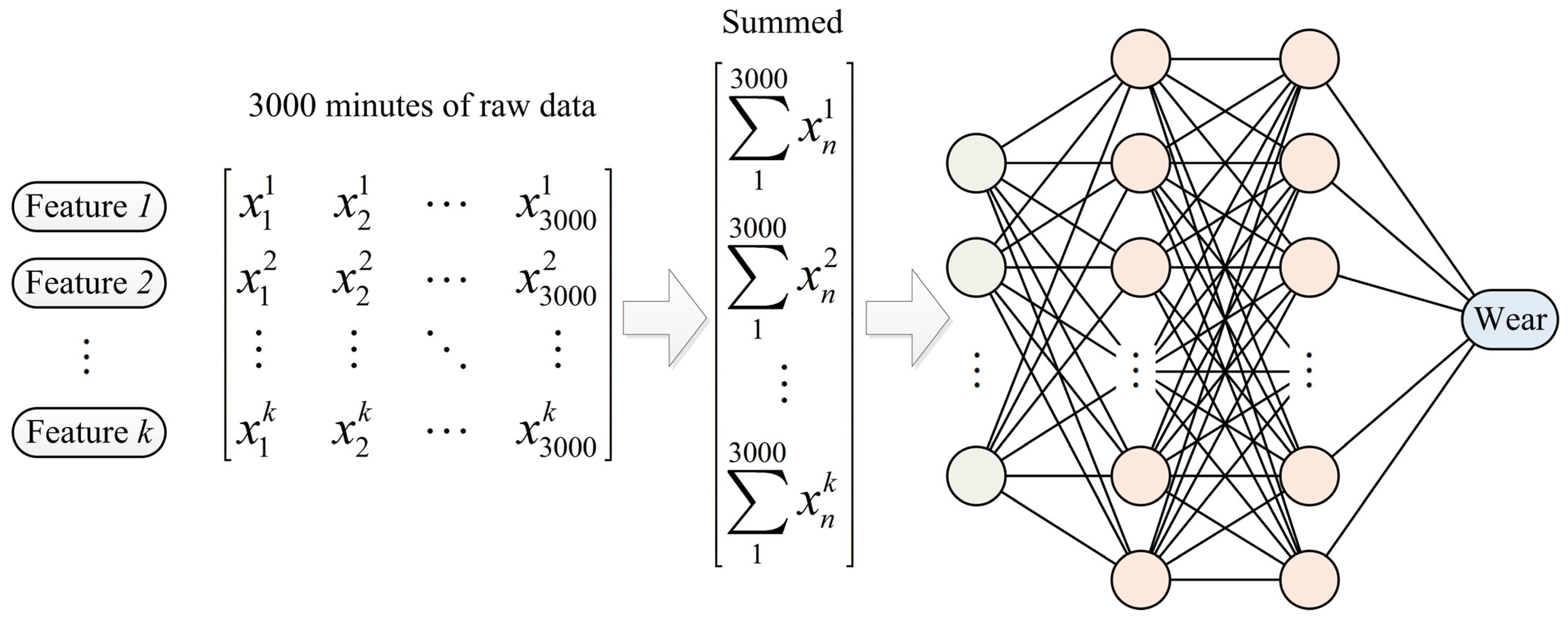
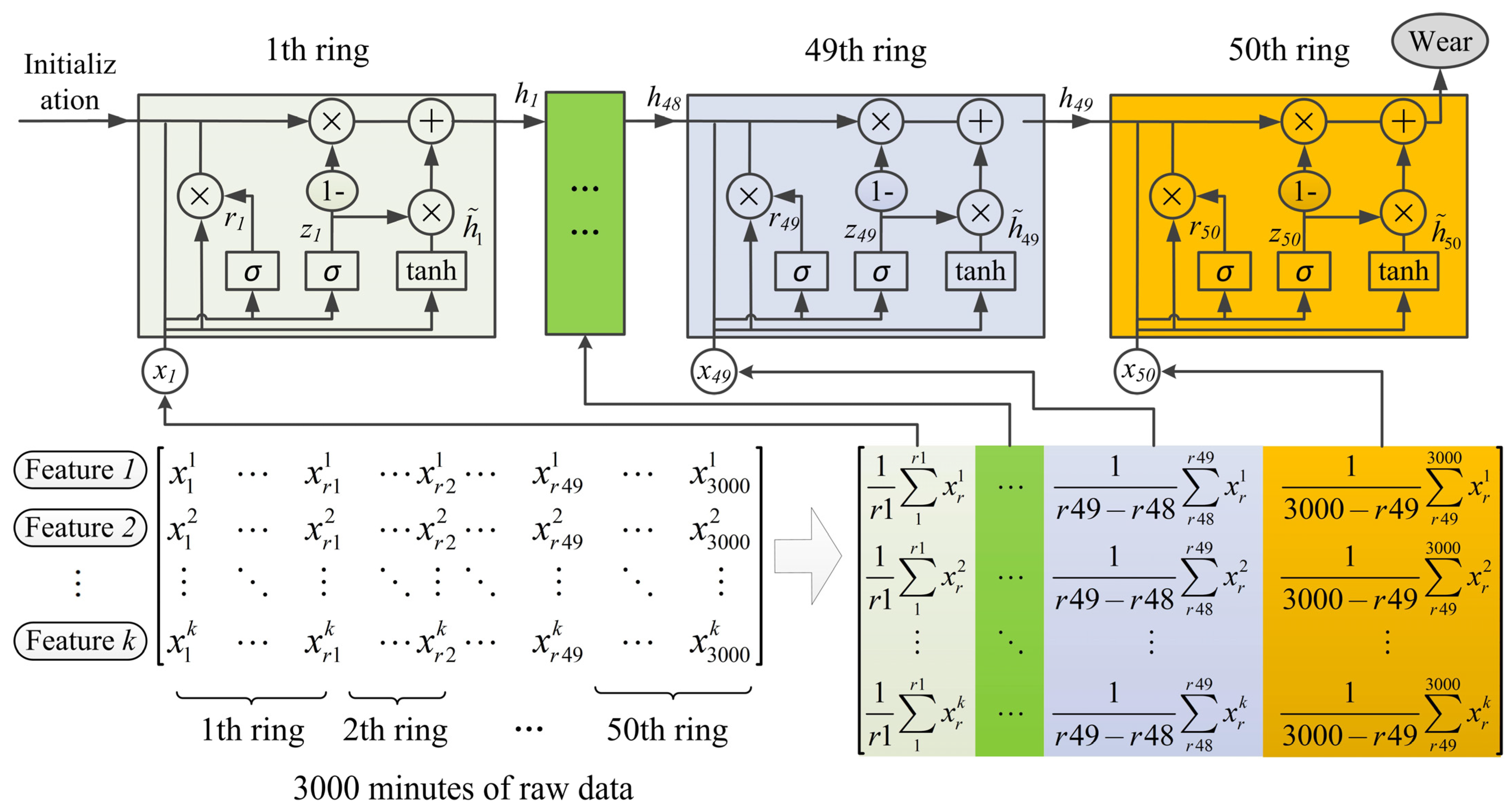
Previous research has provided valuable insights, yet limitations persist. (1) The parameters used as model inputs are derived from theoretical studies and empirical formulas. However, current shield tunneling parameters are sourced from onsite monitoring systems, encompassing over 171 features such as grouting amount, foam system, advance jack oil pressure, synchronized grouting pressure, shield tail seal grease compartment pressure, etc. Apart from the explicit influencing factors, there may also be parameters that indirectly exert significant impacts on disc cutter wear. (2) The limitations of different models stem from their structural characteristics, making it unreasonable to apply the same preprocessing methods to heterogeneous data and models. For instance, in classical ML models, the common practice is to simply average shield operation parameters; this approach may ignore the effects of short-term extremes. By contrast, time series models use a sliding window input format that can alleviate this oversight. Therefore, further research is necessary to explore the optimal combination of input data obtained through various preprocessing techniques paired with different prediction models.

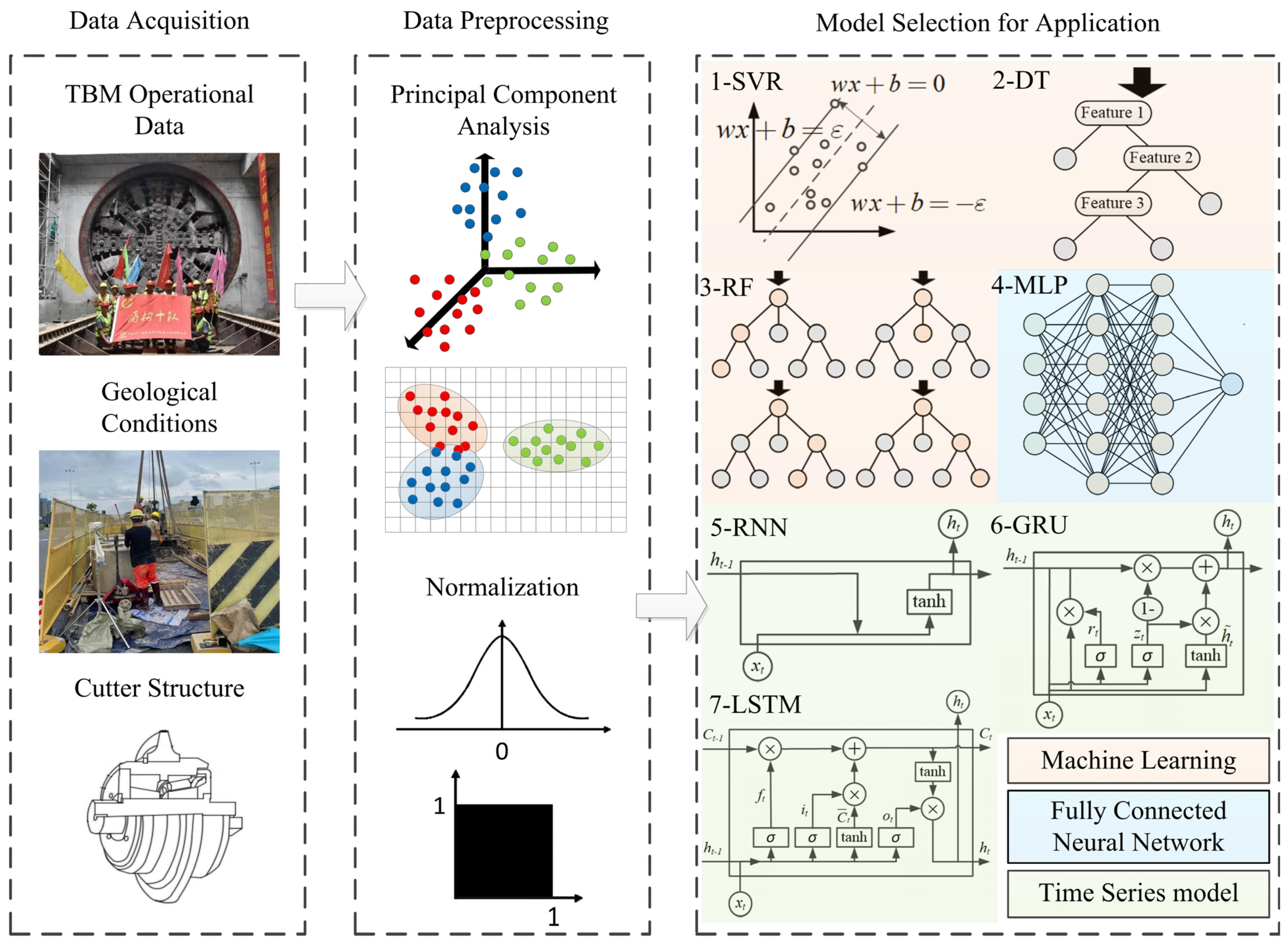
In this study, we explore the practical approach for predicting disc cutter wear by combining various normalization and dimensionality reduction methods with multiple machine learning and recurrent neural networks based on a practical case project in Guangzhou, China.

2. Background and Methodology

2.1. Problem Description

This study uses the tunneling data from line 18 of Guangzhou Metro, which is located on the coast of the Pearl River Delta of Guangdong, China. Line 18 starts from Wangqingsha Station in Nansha District to Guangzhou Dong Railway Station in Tianhe District. The total length is 61.3 km. It was designed to have nine stations with an average distance of 7.6 km between two adjacent stations. The maximum distance between the two stations is 25.9 km, while the minimum is 2.3 km, as shown in Figure 1.

The segment investigated in this study is located between Nancun Wanbo and Panyu Square stations. The total length of the line studied is 3413.7 m, with the left metro line having a length of 1703.0 m and the right metro line having a length of 1710.7 m. Before excavations, geological surveys were carried out to investigate the features of different layers [29]. Figure 2 depicts the geology of Guangzhou as complex as the karst geology. The geological environment is also difficult for tunneling. The analyzed section goes through the geological layers containing granite-weathered layers in slightly, moderately, or highly weathered conditions.

Through UCS testing of samples from the borehole, it was found that the UCS of slightly weathered granite ranged from 44.9 to 101.6 MPa, marking a significant increase compared to that of moderately weathered granite, which ranged from 21.2 to 36.7 MPa. The geological differences affecting some operational features, for example, the cutter head torque and force on the right metro line, change when switching between granite types, as shown in Figure 3. Thus, the UCS is a non-negligible factor when discussing disc wear in this project.

This structure is the same in the TBM of the right metro line and the left metro line. Each cutter head contains 59 cutters in two sizes. S1–S12 cutters are 17 inches, and the other S13–S58AB cutters are 19 inches. Figure 4 shows a schematic section of the cutter head and disc cutter arrangements of the shield. The TBM has a length of 12.94 m, and the cutter head has a diameter of 8.84 m.

The field data are acquired from the monitors in the TBM every minute. These data specifically include thrust force (TF), cutter head torque (CT), penetration depth (PD), cutter head rotation speed (CRS), etc. The TBM field monitors categorize the working states into “Excavation”, “Segments”, and “Shutdown” when collecting data. For this study, data from the two tunnels were collected for more than 50,000 min in the “Excavation” states, encompassing a total of 263 features, and Figure 3 shows some of the shield operation parameters concatenated in series under this state. The geological exploration, operational data collection, and cutter structure constitute the three main aspects that affect the extent of cutter wear [18,30,31]: (1) the geological conditions (e.g., UCS, CAI); (2) real-time TBM performance parameters (e.g., CT, PD, CRS); and (3) cutter structure (e.g., dimensions and placing).

2.2. Research Method

Data preprocessing is placed in the first place to guarantee the quality of the dataset before model training. The following step is to divide the dataset into training, validation, and testing sets, which are used for training and evaluating TBM cutter wear prediction models.

The prediction models in this study can be classified into three kinds: (1) traditional machine learning algorithms, including SVR, decision tree (DT), and random forest (RF); (2) fully connected neural networks (multilayer perceptron, MLP); and (3) time series models, including recurrent neural networks, long short-term memory models (LSTMs), and GRUs. Among these models, some model metrics are used to evaluate the model’s performance. The flowchart of this study is displayed in Figure 5.

Among the aforementioned 7 models, constrained by their structures, the input forms of data can be categorized into two major types. The first type includes machine learning and fully connected neural networks, in which input data are relatively discrete and need to be represented as a set of feature vectors. The second type is the time series model. Compared with the input of the first category of models, this type of model adds the time information of the input data. In actual excavation, the shield tunneling process is a continuous operation, and the wear of the disc cutter is continuously generated as the TBM advances. Therefore, for the first model type, the disc cutter wear data needs to be summed and averaged before being used as input. Below, take the input of MLP as an example: a disc cutter experiences a shield excavation at a distance of 50 rings (assuming 3000 min) under the action of [Feature 1, Feature 2, Feature 3, …, Feature k] (each feature is collected at a frequency of once per min), and its wear increases from 10 mm to 14 mm. Therefore, before inputting, it should sum and average the 3000 data points, and the corresponding Y label is 4 mm, as shown in Figure 6.

Such a processing method may be undesirable because it will ignore the data of certain special cases in the continuous signal. In comparison, time series models can better reflect the actual tunneling and disc cutter wear processes. This study employs three time series models, the RNN, LSTM, and GRU, respectively. Among them, the RNN is the basic recurrent neural network architecture [32]; LSTM solves the gradient vanishing problem of the RNN by introducing the input gate, forget gate, output gate, and cell state. It has long-term memory ability and is suitable for processing long sequence data, but the computational complexity is high [33]. GRU merges the forget gate and input gate of LSTM into an update gate, sets up a reset gate, removes the cell state, simplifies the model structure, and reduces the computational complexity [34,35]. Hyperparameters are critical prerequisites that determine model performance. In this work, we focus on evaluating the interaction between different preprocessing methods and models; accordingly, all time series models were configured with a single hidden layer and the tanh activation function. For each model, four settings of hidden layer node numbers (64, 128, 258, and 512) were explored. Combined with the data characteristics of this project, with GRU as an example, the format of the input data for the time series models is shown in Figure 7.

Time series models, owing to their sliding window input format, can retain considerably more consecutive shield operation information than the models discussed above. Nevertheless, using the raw shield parameters directly is impracticable. Take the right line as an example. More than 25,000 valid data were collected for each parameter, whereas only 11 corresponding geological records exist, yielding a pronounced imbalance of approximately 2290:1 between dense shield operation data and geological data. Directly inputting these data into the network would risk causing the model to overlook the influence of geological conditions on disc cutter wear, an effect that is crucial and cannot be disregarded. Thus, to enable the model to recognize disc cutter wear as a continuous process while preventing crucial factors (geological and cutter structural parameters) from being obscured by discrepancies in data volume, we adopt a ring-based summation averaging strategy, as defined in Equation (1).

$$x_n={\displaystyle \frac{1}{rn-r(n-1)}}{\displaystyle \sum _{r(n-1)}^{rn}{x}_r^k}$$

(1)

where rn represents the end time of each excavation ring.

Based on the aforementioned assumption, raw data with a distance of 50 rings (assuming 3000 min) can be transformed into a [k × 50] input matrix. Each column of this matrix corresponds to the operational parameter’s status of one excavation ring, and they are sequentially input to the GRU model as time steps according to the actual shield occur. The disc cutter wear is the result of the combined effects of the preceding 50 time steps. During GRU training, the update gate (z_n) and the reset gate (r_n) are first calculated according to Equations (2) and (3). The outputs of these gates will control the update of the hidden state and the retention of historical information.

$$z_n=\sigma (W_z\cdot [h_{n-1},x_n]+b_z)$$

(2)

$$r_n=\sigma (W_r\cdot [h_{n-1},x_n]+b_r)$$

(3)

where W_z, b_z, W_r, and b_r are the parameter matrix and bias vector of the update gate and reset gate, respectively; h_n−1 is the hidden state of the previous excavation ring; x_n is the shield parameter of the current ring; and σ is the Sigmoid activation function.

Then, GRU uses the reset gate to control the dependence on the previous hidden state and calculates the candidate hidden state as follows:

$${\tilde{h}}_n=\tanh (W\cdot [r_n\cdot h_{n-1},x_n]+b)$$

(4)

The last step combines the update gate to calculate the hidden state passed to the next step as follows:

$$h_n=z_n\cdot h_{n-1}+(1-z_n)\cdot {\tilde{h}}_n$$

(5)

3. Data Preprocessing

Data preprocessing contains the following basic steps. (1) Drop out the feature columns containing more than 10% of missing data. (2) Use the linear interpolation method to fill the missing data. (3) Use PCA to reduce the dimension of features with the same meaning but collected in different sensors. (4) Use different scalers to transform the feature data. The scales include the Min Max Scaler, standardization, and Max Absolute (Max Abs) Scaler. (5) Integrate the features of TBM operational data (field data), geological features, and cutter information to generate the merged dataset. (6) Divide the dataset into a training dataset, validation dataset, and testing dataset.

3.1. Data Analysis

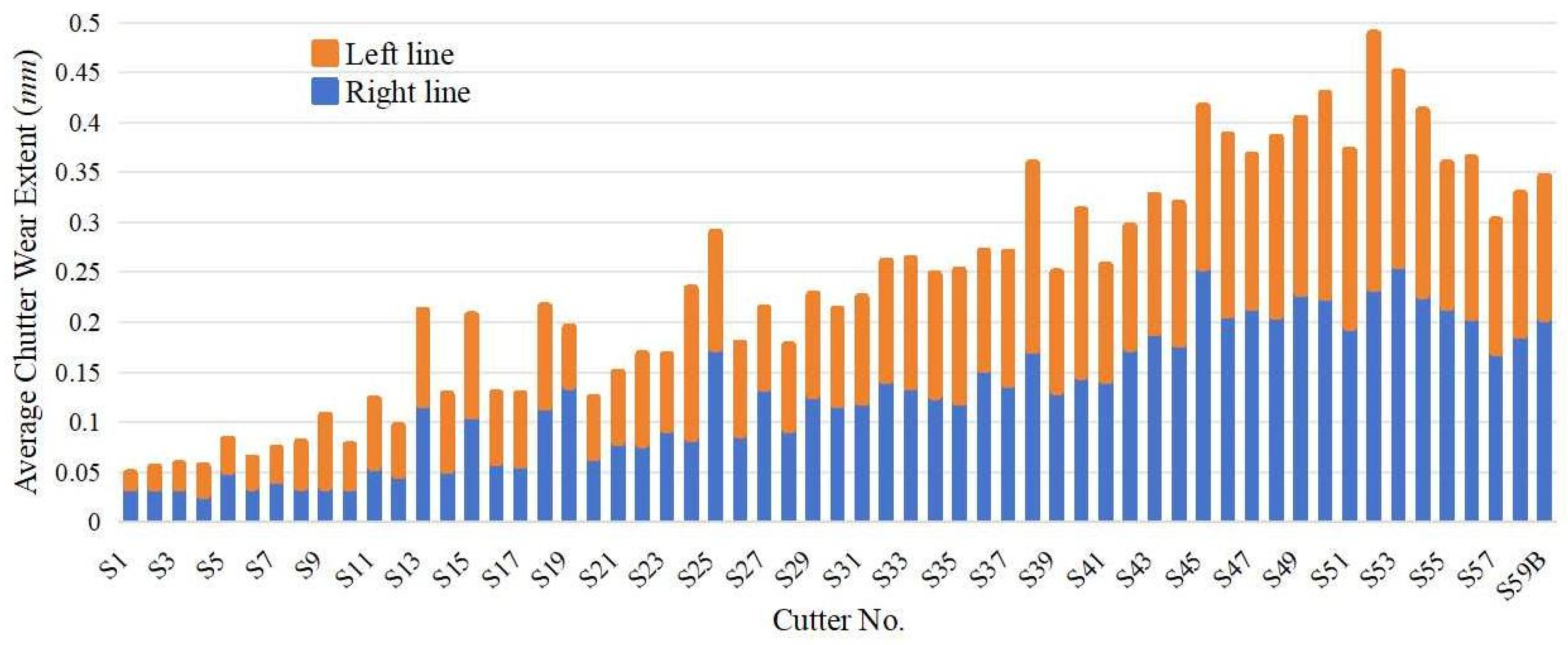
By organizing the information about cutter wear in both the right and left lines, we have compiled a total of 886 wear measurement records. Among these, there are only a few instances of abnormal cutter wear, specifically 26 records. Among the 26 abnormal wear records, nearly 20 involve the double-edged disc cutters installed around the center of the cutter head. Owing to their small gyration radius, these cutters undergo both sliding and rolling motions and are subjected to large axial forces, which leads to uneven wear of the cutter rings. Because wear measurement can only be taken manually when the TBM shuts down, it is impossible to determine the exact moment or precise position at which the abnormal wear occurs. To avoid the imbalance between normal and abnormal wear records from interfering with subsequent model training, we have excluded these data points from further analysis.

Figure 8 illustrates the average cutter wear extent in two lines. The average cutter wear extent is calculated as the average extent of the interval between cutter wear measurements. The cutters near the center of the cutter head are less likely to be worn than the others in the outer cutter head. The original wear extent is used as a predictive variable in the time series model, and the average wear extent is used in traditional machine learning and MLP models.

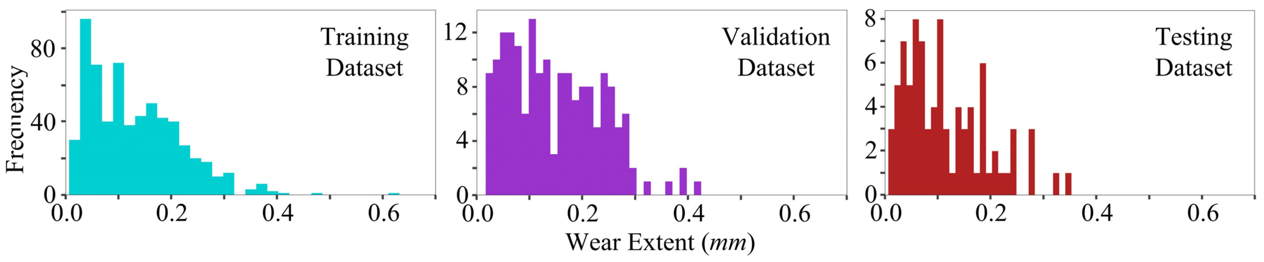
To avoid model overfitting and estimate the performance, we simulate the real scenario of the TBM excavation process; the last two measurements of the cutter wear extent results are extracted and treated as a testing dataset. The remaining data are randomly divided into training datasets and validation datasets. The ratio of the training dataset, validation dataset, and testing dataset is about 7:2:1. Figure 9 displays the average cutter wear extent distributions for the training, validation, and testing datasets based on the aforementioned statistics. The wear in all three datasets is predominantly concentrated in the 0~0.3 mm range with consistent peaks, while a small number falls within 0.3~0.5 mm. Their distribution shapes and frequency scales closely match, indicating that the data split maintained distributional consistency and thus provided a solid foundation for fair model performance evaluation.

3.2. Operation Parameter Feature Reduction

There are 171 features in the parameters of the TBM excavation operation. Initially, features with missing data exceeding 10% of the entire dataset are removed, leaving 110 features. The operational parameters are collected once every minute by sensors distributed across various key components of the TBM, with sensors on each component categorized into groups. Due to the influence of complex working conditions, information collected by the sensors may inevitably have missing values. To address this issue, we employ the linear interpolation method to fill in the missing data. These remaining 110 features primarily originate from 18 sensor groups. To enhance the prediction model to better focus on core features, we further utilize PCA for dimensionality reduction in the current operational features.

As a Karhunen–Loeve transformation, PCA is also widely used in feature selection [36]. It transforms n vectors in a d-dimensional space (x₁, x₂, …, x_n) into n new vectors, which are in a new d′-dimensional space (x′₁, x′₂, …, x′_n) as follows:

$${x^{\prime }}_i={\displaystyle {\sum }_{k=1}^{d^{\prime }}{a}_{k,i}{e}_k},d^{\prime }\le d$$

(6)

where e_k is the eigenvectors corresponding to the d′ largest eigenvalues λ_k for the scatter matrix S and a_k,i are the projections of the original vector x_i on the eigenvectors e_k. The calculation of the scatter matrix can be defined as follows:

$$S=E\left[x_i{x}_j^T\right], \mathrm{for} i = 1 \mathrm{to} n$$

(7)

Generally, the cumulative explained variance should be up to 80% after PCA. The PCA scaler first fits the data in the training dataset and validation dataset. The scaler later transforms the whole dataset to reduce dimensions. After transformation, feature group data are merged together as the new dataset. The PCA features dimension reduction result is shown in

Table 1. The PCA result of each feature group.

No.	Feature Groups	Num. of Features	Num. of PCA Components	Explained Ratio (%)
1	Grouting amount	3	1	96.79
2	Real-time accumulation of loop mixture	6	1	99.75
3	Real-time accumulation of air	6	1	93.76
4	Foam system	2	1	99.97
5	Horizontal and vertical trend	2	1	91.95
6	Earth pressure	6	1	93.06
7	Advance jack oil pressure	6	2	85.11
8	Synchronized grouting pressure	3	1	81.62
9	Shield tail seal grease front compartment pressure	10	2	91.75
10	Shield tail seal grease middle compartment pressure	10	2	94.36
11	Shield tail seal grease rear compartment pressure	10	2	91.07
12	Grouting channel grouting times	2	1	90.50
13	Main bearing outer seal grease (EP2) grease counter	2	1	97.70
14	Advance jack stroke	6	2	98.71
15	Articulating cylinder stroke	4	2	82.17
16	Front tail shield horizontal and vertical deviation	4	1	94.23
17	Front rear shield coordinates	6	1	99.59
18	Shield front and rear mileage	2	1	99.99

.

3.3. Data Normalization

Previous research has shown that different data normalization methods have different effects on data analysis [37]. However, few studies discuss different data normalization methods on TBM data. To fully use the information of the original dataset and avoid the effects of data normalization methods, three methods are used in this study, including the Min Max Scaler, standardization, and the Max Absolute Scaler.

(1)

The Min Max Scaler method is calculated as follows:

$$X_{transform,i}={\displaystyle \frac{X_{original,i}-{\stackrel{\min }{X}}_{original,i}}{{\stackrel{\max }{X}}_{original,i}-{\stackrel{\min }{X^{\prime }}}_{original,i}}}, \mathrm{for} i = 1 \mathrm{to} d \mathrm{or} d^{\prime }$$

(8)

where i denotes each feature in vector X.

(2)

Similarly, the standardization method is calculated as follows:

$$X_{transform,i}={\displaystyle \frac{X_{original,i}-{\overline{X}}_{original,i}}{sd({X^{\prime }}_{original,i})}}, \mathrm{for} i = 1 \mathrm{to} d \mathrm{or} d^{\prime }$$

(9)

(3)

And the Max Absolute Scaler method is calculated as follows:

$$X_{transform,i}={\displaystyle \frac{X_{original,i}}{{\stackrel{\max }{X^{\prime }}}_{original,i}}}, \mathrm{for} i = 1 \mathrm{to} d \mathrm{or} d^{\prime }$$

(10)

In addition, the direct PCA method is also applied in the feature dimension reduction directly instead of the above feature groups.

Table 2. Directly PCA for Dimension Reduction.

Norm. Method	Num. of Components	Total Explained Variance Ratio (%)
Min Max	14	91.01
Standardization	16	88.90
Max Abs	14	89.29

lists the explained variance ratios for the selected components and the scree plots as shown in Figure 10. Under the same normalization, the geological and cutter geometry features are merged into datasets.

4. Method Performance and Comparison

In this study, we utilize an SVR with an RBF kernel function and an RF algorithm where the maximum depth of the tree is explored between 10 and 21, and the minimum sample split parameter ranges from 2 to 5, to predict the extent of cutter wear. Additionally, traditional neural networks (MLP) and time series neural network models (RNN, LSTM, and GRU) are employed for learning and predicting the disc cutter wear. It is worth noting that while the predictive variable used in the time series model is the wear extent between measurement intervals, the predictive variable used in traditional machine learning algorithms (SVR, RF, and MLP) is the average cutter wear in the corresponding interval.

To verify the performance of the models, the coefficient of determination R² and the mean absolute percentage error (MAPE) describe the error between the predicted and actual values.

$$R^2=1-{\displaystyle \frac{{\displaystyle {\sum }_i}{(wea{r}_i-{wear}_i^{\prime })}^2}{{\displaystyle {\sum }_i}{(wea{r}_i-{\overline{wear}}_i)}^2}}$$

(11)

$$MAPE={\displaystyle \frac{1}{N}}{\displaystyle \sum _{i=1}^N\left|\frac{wea{r}_i-{wear}_i^{\prime }}{wea{r}_i}\right|}\times 100\%$$

(12)

where wear_i represents the actual wear value, ${wear}_i^{\prime }$ is the predicted wear value of the model, $\overline{wear}$ represents the average of the actual wear values, and N is the number of samples in the training or test dataset. R² represents the proportion of the total variance in wear explained by the model; the closer R² is to 1, the better the wear predictions. The MAPE measures the mean absolute percentage error of those predictions; the smaller the MAPE, the more accurate the wear forecasts.

Traditional machine learning algorithms are performed on an ACER E5-572G-528R laptop with an i5-4210M CPU, 2.60 GHZ, and 8.00GB of RAM memory. Neural networks are run in the cloud server AutoDL with an E5-2680 v4@ CPU, 2.40 GHz, 20 GB of memory, and a 12 GB RTX 3060 GPU.

4.1. Traditional Machine Learning

In this section, we attempt to establish a predictive model by three traditional machine learning models (SVR, DT, and RF) and test their performance under different datasets and normalization methods. Among them, with SVR using RBF kernel’s best hyperparameters, the value of “C” tends to be large and “gamma” tends to be small; the optimal hyperparameters for DT and RF are “max_depth = 20, min_samples_split = 5”, and “max_depth = 10, min_samples_split = 5, n_estimators = 60”, respectively. Different models’ model metrics are listed in

Table 3. Average model metric of different models.

Model	Train R2	Train MAPE	Valid R2	Valid MAPE	Test R2	Test MAPE
RBFSVR	0.40	0.76	0.37	0.62	0.37	0.97
Decision Tree	0.85	0.19	0.02	0.48	−0.10	0.67
Random Forest	0.81	0.26	0.43	0.39	0.47	0.54

.

As shown in Table 3, (1) random forest ranks first among these methods. (2) Although the decision tree outperforms random forest on the training dataset, the performance of decision tree even is worse than the average model (i.e., R² less than 0 on the testing dataset). Therefore, further exploration of the random forest model metric of different datasets under three kinds of normalization is listed in

Table 4. Model metric of random forest.

Dataset	Normalization	Train R2	Train MAPE	Valid R2	Valid MAPE	Test R2	Test MAPE
Raw	Max Abs	0.80	0.26	0.44	0.39	0.47	0.55
	Min Max	0.80	0.27	0.44	0.39	0.46	0.55
	Standard	0.80	0.27	0.44	0.39	0.46	0.55
PCA	Max Abs	0.80	0.26	0.38	0.41	0.43	0.51
	Min Max	0.80	0.26	0.39	0.40	0.45	0.52
	Standard	0.81	0.25	0.44	0.39	0.46	0.55
PCA directly	Max Abs	0.81	0.26	0.48	0.39	0.50	0.53
	Min Max	0.82	0.25	0.44	0.39	0.49	0.54
	Standard	0.83	0.25	0.45	0.39	0.47	0.55

.

As shown in Table 4, the (1) PCA directly dataset outperforms the other two datasets across three normalization methods, and the performance of the PCA dataset is the worst. (2) For normalization methods, no obvious difference between test R² and test MAPE is found within these three datasets.

4.2. Neural Networks

The MLP models train various kinds of datasets, and the validation datasets are used as the model’s early stopping criterion. Different hidden layer numbers and activation functions are the hyperparameters of these models.

Table 5. Running time of MLP models with two hidden layers (s).

Dataset	Normalization	Num. of Hidden Layers	Activation Function	Epoch	Total Training Time	Inference Time
Raw	Max Abs	8 × 8	linear × linear	1475	4.393	0.0003
	Min Max	8 × 8	linear × linear	1481	4.287	0.0003
	Standard	64 × 64	relu × relu	1423	4.433	0.0004
PCA	Max Abs	32 × 16	relu × linear	1496	4.757	0.0004
	Min Max	8 × 32	relu × relu	1091	3.511	0.0004
	Standard	64 × 32	relu × relu	1460	4.540	0.0004
PCA directly	Max Abs	64 × 32	relu × relu	1496	4.910	0.0004
	Min Max	64 × 32	relu × relu	1490	5.315	0.0005
	Standard	8 × 32	relu × relu	1492	4.886	0.0004

lists the running time of two hidden layer MLP models, whose test R² ranks first in all the hyperparameter settings. (1) Under Max Absolute or Min Max Scaler, MLP on the raw dataset fits the training dataset with a smaller number of hidden layers than the other dataset (i.e., PCA, PCA directly). (2) The PCA dataset requires fewer epochs and less time to fit the data.

The model metrics of MLP models, as shown in

Table 6. Model metric of MLP models with two hidden layers.

Dataset	Normalization	Num. of Hidden Layer	Train R2	Train MAPE	Valid R2	Valid MAPE	Test R2	Test MAPE
Raw	Max Abs	8 × 8	0.438	0.576	0.433	0.508	0.545	0.648
	Min Max	8 × 8	0.439	0.577	0.423	0.497	0.539	0.667
	Standard	64 × 64	0.537	0.424	0.479	0.370	0.576	0.486
PCA	Max Abs	32 × 16	0.505	0.508	0.454	0.439	0.547	0.568
	Min Max	8 × 32	0.437	0.520	0.441	0.443	0.571	0.573
	Standard	64 × 32	0.539	0.443	0.470	0.383	0.563	0.555
PCA directly	Max Abs	64 × 32	0.499	0.520	0.450	0.454	0.550	0.549
	Min Max	64 × 32	0.500	0.507	0.450	0.454	0.547	0.598
	Standard	8 × 32	0.502	0.507	0.463	0.436	0.576	0.604

, indicate several observations. (1) Under standardization, the models generally achieve better R² values compared to other normalization methods. However, not all the corresponding MAPE values are the smallest. (2) Unlike the raw dataset, the other three kinds of datasets require more neurons in the hidden layer to effectively fit the dataset. (3) With standardization, both the raw dataset and PCA dataset exhibit the best performance among these models. However, as seen from the above table, the PCA dataset takes less time to train the model.

4.3. Time Series Model

We evaluate time series models with different structures and hyperparameters on various datasets under three types of normalization, as detailed in Appendix A. For each experimental configuration, an early stopping mechanism was implemented: training will terminate if model performance fails to improve for 10 consecutive epochs.

Table 7. Running time of time series models (s).

Dataset	Normalization	Model	Num. of Hidden Layers	Epoch	Total Training Time	Inference Time
Raw	Max Abs	LSTM	512	1301	51.345	0.0109
	Min Max	GRU	256	694	26.652	0.0108
	Standard	RNN	256	700	23.959	0.0092
PCA	Max Abs	GRU	64	2916	93.335	0.0082
	Min Max	GRU	256	918	27.775	0.0099
	Standard	RNN	512	315	11.511	0.0109
PCA directly	Max Abs	GRU	256	1076	41.575	0.0107
	Min Max	LSTM	128	818	31.590	0.0112
	Standard	GRU	512	190	7.715	0.0110

and

Table 8. Model metric of time series models.

Dataset	Normalization	Model	Num. of Hidden Layers	Train R2	Train MAPE	Valid R2	Valid MAPE	Test R2	Test MAPE
Raw	Max Abs	LSTM	512	0.726	0.421	0.773	0.389	0.700	0.506
	Min Max	GRU	256	0.717	0.423	0.784	0.383	0.702	0.479
	Standard	RNN	256	0.760	0.367	0.652	0.390	0.658	0.507
PCA	Max Abs	GRU	64	0.750	0.391	0.773	0.391	0.672	0.497
	Min Max	GRU	256	0.765	0.417	0.801	0.377	0.712	0.471
	Standard	RNN	512	0.733	0.448	0.659	0.440	0.686	0.545
PCA directly	Max Abs	GRU	256	0.752	0.421	0.781	0.411	0.695	0.505
	Min Max	LSTM	128	0.735	0.415	0.775	0.391	0.685	0.490
	Standard	GRU	512	0.717	0.420	0.765	0.389	0.674	0.495

list the running time of these models that achieved the best score on the testing dataset after model fitting and evaluation using the validation dataset. (1) As for the training time, standardization methods use less time than the other two normalization methods. (2) PCA directly takes less time than the other three datasets for model fitting. (3) The training time of the time series model is longer than that of the ANN model listed above.

Table 8 lists the model metrics of the time series models with the best score on the testing dataset after model fitting and evaluation using the validation dataset. (1) The R² value of the time series model is greater than the R² of the MLP model and traditional machine learning model. The test MAPE of the time series model is better than that of MLP. These two results mean the predictive performance of the time series model is superior to the other two types of models. (2) The models using a standardization scaler perform worse than the other two methods in the time series model. This result is different from the MLP model. (3) The performance of the GRU model to fit and predict the cutter wear extent is usually better than the other two time series models. (4) The PCA dataset achieves the best performance under the Min Max Scaler with the GRU model. The R² of the model is 0.712, and the MAPE is 0.471. The other three datasets cannot predict the cutter wear extent to achieve the R² metric value greater than 0.710. The second-best performance is achieved by the raw dataset under the Min Max Scaler.

4.4. Comparison and Discussion

Based on the comparison of various dataset dimensions, normalizations, and models, the result shows that the time series models proved to be an effective model to predict the cutter wear extent. Feature size cannot always correlate with the model training time. The feature size is raw > PCA > PCA directly. For the time series models, the PCA directly dataset takes the least time for model training, but the raw dataset does not take the longest time. Similar patterns also emerge in MLP models. Generally, raw datasets take the longest time to train when using machine learning models or MLP. This rule breaks in the time series model, which can be a result of information loss in feature dimension reduction. The reduced feature sometimes needs more epochs or hidden layer numbers for model training.

There are three kinds of dimension reduction strategies. Among these strategies, the PCA dataset has high interpretations of the feature, as this method keeps all the features. However, the PCA datasets seldom achieve better performance than the other two strategies. The PCA directly dataset has the poorest explainability of the feature since the components are calculated according to the covariance matrix.

The most proper normalization methods for models are different. MLP models predict the cutter wear extent well under standardization methods. However, the Max Absolute Scaler is more proper than standardization for time series models, even though the model trains the dataset under the standardization method more quickly.

The model with a large value of R² does not always result in a small value of the MAPE. Take Table 8 as an example. In the PCA dataset, the model obtains the highest R² under Min Max normalization but the smallest MAPE under Max Absolute normalization. This phenomenon results from different scales of each cutter’s wear extent in the denominator of Equation (12). MLP and the time series neural network have proved to be more effective than the traditional machine learning models. In the hidden layer, different interactions of input features are calculated to predict the cutter wear extent. As Shahrour et al. [1] discuss, the potential mechanism under these interactions still needs to be figured out.

5. Conclusions

This project focuses on regression prediction for disc cutter wear in TBM using Guangzhou Metro Line 18 data, aiming to reduce inspection and replacement costs while preventing cutter head damage. This study improves soft computing models by exploring feature dimension reduction and normalization and comparing model performance across traditional ML, MLP, and time series neural networks. Based on the results, the main conclusions of this study can be summarized as follows:

(1)

The results indicate that all the time series models have proven to be more effective than traditional machine learning models and fully connected neural networks in predicting the extent of cutter wear. The PCA + Min Max + GRU yielded the best results (R² = 0.712, MAPE = 0.471), surpassing the strongest RF and MLP baselines by 42% and 24%, respectively.

(2)

Min Max normalization applied to either the raw or the PCA data consistently yielded the best or second-best predictive accuracy. Max Abs scaling provided stable but rarely top-ranking results, whereas standardization tended to cause overfitting in a large number of neuron models.

(3)

All experimental models achieve inference times on the order of milliseconds, rendering runtime differences negligible for engineering applications. Nevertheless, the GRU model trained on the PCA-compressed feature set retained the highest accuracy while reducing the input dimensionality by 86%, thereby simplifying downstream storage and deployment.

(4)

A hidden-state size of 256 consistently provided the best trade-off between accuracy and generalization across the tested time series models, whereas enlarging it to 512 offered no further gain. Because a disc cutter usually advances no more than roughly 200 rings in a single service cycle, 256 units are sufficient for the network to capture all influential information throughout the cutter’s entire operational life.

The geological condition of Guangzhou Metro Line 18 is simple and only contains three kinds of granite-weathered layers. In the future, more datasets need to be merged to train a more stable model that can be widely used.