Fatigue Predictive Modeling of Composite Materials for Wind Turbine Blades Using Explainable Gradient Boosting Models

Abstract

Wind turbine blades are subjected to cyclic loading conditions throughout their operational lifetime, making fatigue a critical factor in their design. Accurate prediction of the fatigue performance of wind turbine blades is important for optimizing their design and extending the operational lifespan of wind energy systems. This study aims to develop predictive models of laminated composite fatigue life based on experimental results published by Montana State University, Bozeman, Composite Material Technologies Research Group. The models have been trained on a dataset consisting of 855 data points. Each data point consists of the stacking sequence, fiber volume fraction, stress amplitude, loading frequency, laminate thickness, and the number of cycles of a fatigue test carried out on a laminated composite specimen. The output feature of the dataset is the number of cycles, which indicates the fatigue life of a specimen. Random forest (RF), extreme gradient boosting (XGBoost), categorical boosting (CatBoost), light gradient boosting machine (LightGBM), and extra trees regressor models have been trained to predict the fatigue life of the specimens. For optimum performance, the hyperparameters of these models were optimized using GridSearchCV optimization. The total number of cycles to failure could be predicted with a coefficient of determination greater than 0.9. A feature importance analysis was carried out using the SHapley Additive exPlanations (SHAP) approach. LightGBM showed the highest performance among the models (R² = 0.9054, RMSE = 1.3668, and MSE = 1.8682).

1. Introduction

Electricity and energy production are increasing rapidly to meet the world’s energy needs. In order to minimize negative consequences, such as global warming, caused by fossil fuels, renewable energy sources are being turned to when alternative energy sources to fossil fuels are sought [1]. Wind power generation is a promising field in terms of its potential and implementation, especially in the long term. Wind energy is supported for reasons such as being a renewable energy source. The total installed wind energy capacity in gigawatts was 1017.20 gigawatts (GW) as of 2023 [2].

A wind turbine is a machine that converts kinetic energy from the wind into electricity [3]. Wind turbine rotors consist of turbine blades. Turbine blades are critical in the process of converting wind kinetic energy into electrical energy. Depending on the aerodynamic performance of the turbine, a large part of the energy efficiency depends on these blades [4].

As mentioned above, the limited reserves of fossil fuels and the increasing environmental risks posed by their carbon emissions have led to a shift toward other energy sources. Renewable energy sources are a sustainable and clean option for meeting energy needs. The scenario in World Wildlife (WWF), The Energy Report [5], states that by 2050, 95 percent of the energy needed on Earth could be provided from renewable sources.

Wind energy has advantages, such as not emitting toxic gases, the energy spent during the establishment phase of wind turbines can be produced in a short time, and less dependence on foreign energy. The disadvantages are that it is dependent on wind availability and generates significant noise [6].

The widespread use of wind energy applications has influenced the design of wind turbine blades to capture more wind and generate more energy, and blades are increasingly produced from longer and more flexible structures. This causes wind turbine blades to be exposed to more loads [7]. The loads acting on wind turbine blades can be classified as aerodynamic, gravitational, centrifugal, gyroscopic, and operational [8]. Aerodynamic load is the type of load produced by the lift and drag of the wing airfoil section, which depends on wind speed, wing speed, surface quality, angle of attack, and yaw [9]. Gravitational loads include the mass of the components [10].

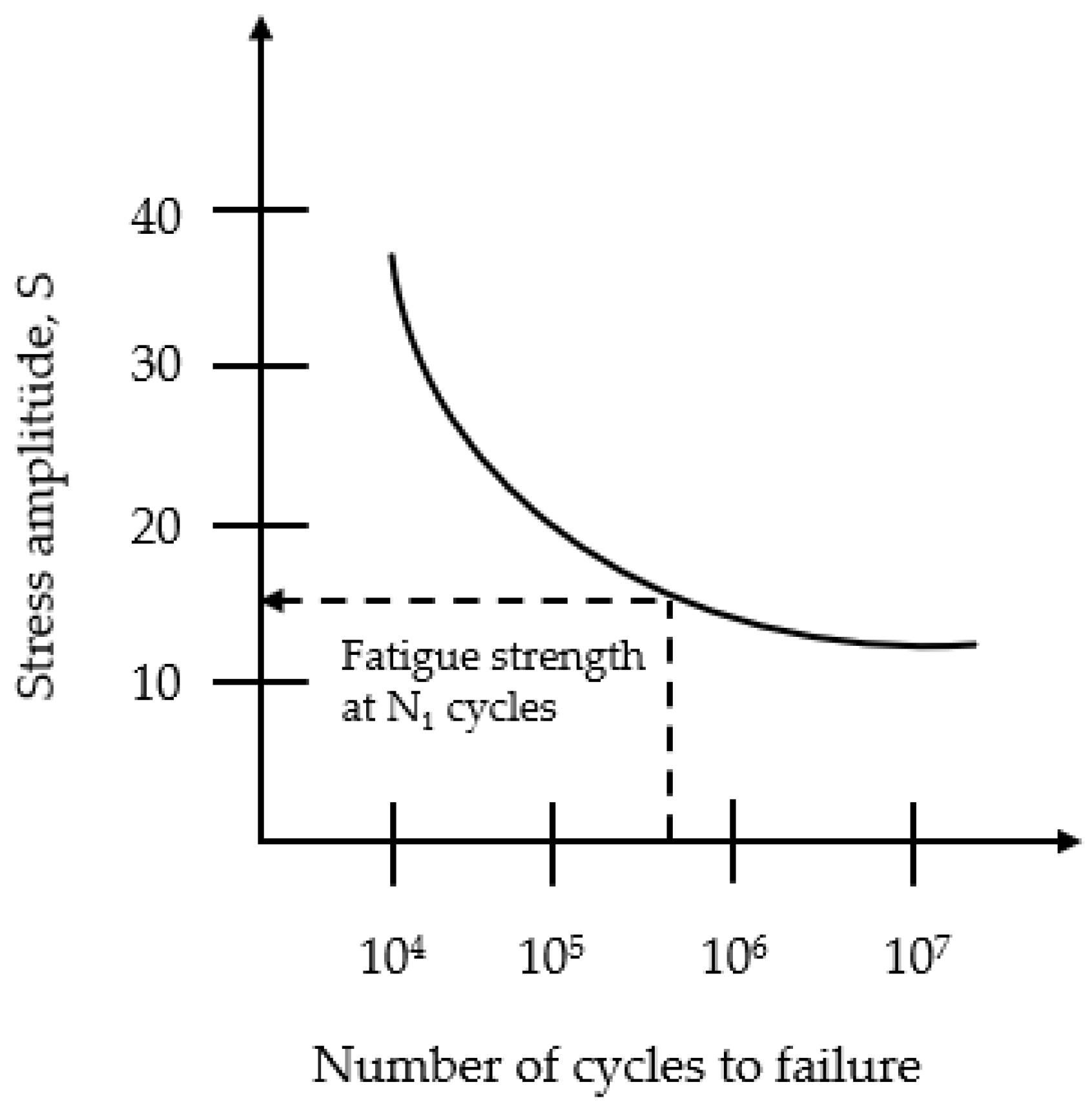
Wind force and inertia forces caused by the rotation of the rotor create a significant load on the wind turbine blades. These forces cause bending and normal stresses in the tower and blades. If the safe limits of the material used are exceeded, structural fractures may occur [7]. Wind turbine blades are subjected to cyclic loading conditions throughout their operational lifetime, making fatigue a crucial consideration in their design. Fatigue often leads to large-scale damage [11].

The wind turbine blades are one of the most prone to damage due to the forces they are subjected to. The main cause of damage to the blades is fatigue in these parts. This type of damage usually occurs at the points where the blades are connected to the root region of the propellers. When subjected to high fatigue loads, these damages occur in shorter periods of time [12]. 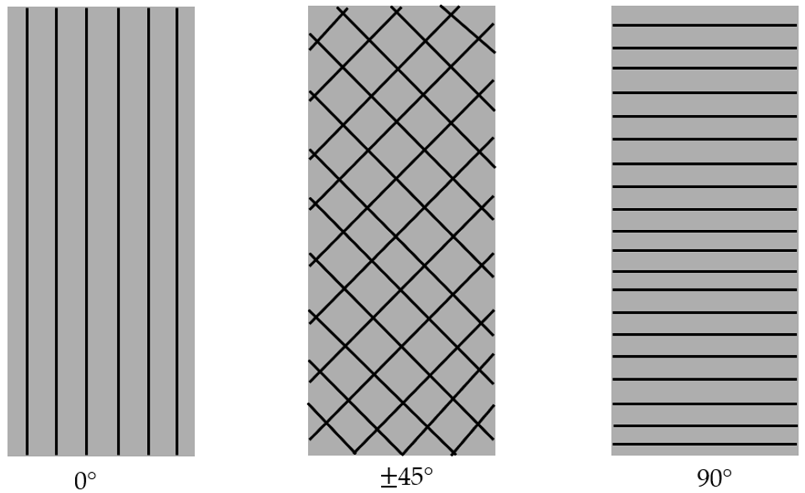Fatigue is mechanical damage to a material or part under dynamic loading [13] and is a phenomenon that affects the wind turbine lifetime. In this study, the number of cycles, which indicates the fatigue life of a specimen, is predicted using the stacking sequence, fiber volume fraction, stress amplitude, loading frequency, laminate thickness, and the number of cycles of a fatigue test carried out on a laminated composite specimen.

The costly and time-consuming nature of experimental tests, the ability to observe the relationships between variables using various statistical methods in data-driven methods, and the ability to develop a general model for different configurations by continuously feeding new data show the practical advantages of using data-driven methods. Fatigue behavior in composite turbine blades can be highly nonlinear and dependent on numerous parameters, such as the stacking sequence. Traditional analytical closed-form models often become cumbersome or less accurate with increasing complexity. On the other hand, data-driven models can capture higher-dimensional, nonlinear interactions more effectively, reducing prediction error and computational cost. This study presents the use of tree-based models and explainable artificial intelligence (XAI) to predict the fatigue life of wind turbine blades. Previous works in the literature usually use artificial neural network (ANN) and support vector regression (SVR) models, but the novelty here is provided by using tree-based models and XAI. In addition, the uniqueness of this study is that there is no other study that examines the fatigue life of composite material (especially the dataset we analyzed) with machine learning methods. Moreover, the proposed method can be easily applied to the real world.

Machine learning is an artificial intelligence (AI) method that is widely used in almost every field today. There are many ML studies on wind turbines and fatigue behavior. Dervilis et al. [14] used the automatic associated neural network (AANN) and radial basis function (RBF) for fault detection of wind turbine blades under continuous fatigue loading. He et al. [15] used support vector regression (SVR) to accurately predict the fatigue loads and power of wind turbines under yaw control. The results obtained demonstrated both the accuracy and robustness of the model. Miao et al. [16] proposed a machine learning model based on the Gaussian process (GP) to predict the fatigue load of a wind farm. The results obtained showed that the GP improved prediction accuracy. Yuan et al. [17] developed a machine-learning-based approach to model the fatigue loading of floating wind turbines. The results showed that the random forest (RF) model provided a prediction accuracy of up to 99.97%, with a minimum prediction error not exceeding 3.9%. Luna et al. [18] trained and tested artificial neural network (ANN) architectures to predict the fatigue of a wind turbine tower using data based on tower top oscillation speed and previous fatigue state. The results obtained are promising. Bai et al. [19] used a residual neural network (ResNet) to predict the fatigue damage of a wind turbine tower at different wind speeds. The results showed that the efficiency of the proposed probabilistic fatigue analysis method can be improved. Santos et al. [20] trained loss function physics-guided learning of neural networks for fatigue prediction of offshore wind turbines. The study demonstrated the potential of the method. Wu et al. [21] used an improved SVR model with gate recurrent unit (GRU) and grid search methodology to predict the fatigue load in the nacelle of wind turbines. The results showed that the proposed model framework can effectively predict the fatigue loads in the nacelle. Ziane et al. [22] used ANN based on back propagation (BP), particle swarm optimization (PSO), and cuckoo search (CS) to predict the fatigue life of wind turbine blades under variable hygrothermal conditions. They used mean square error (MSE) to evaluate the results. CS-ANN achieved the best result.

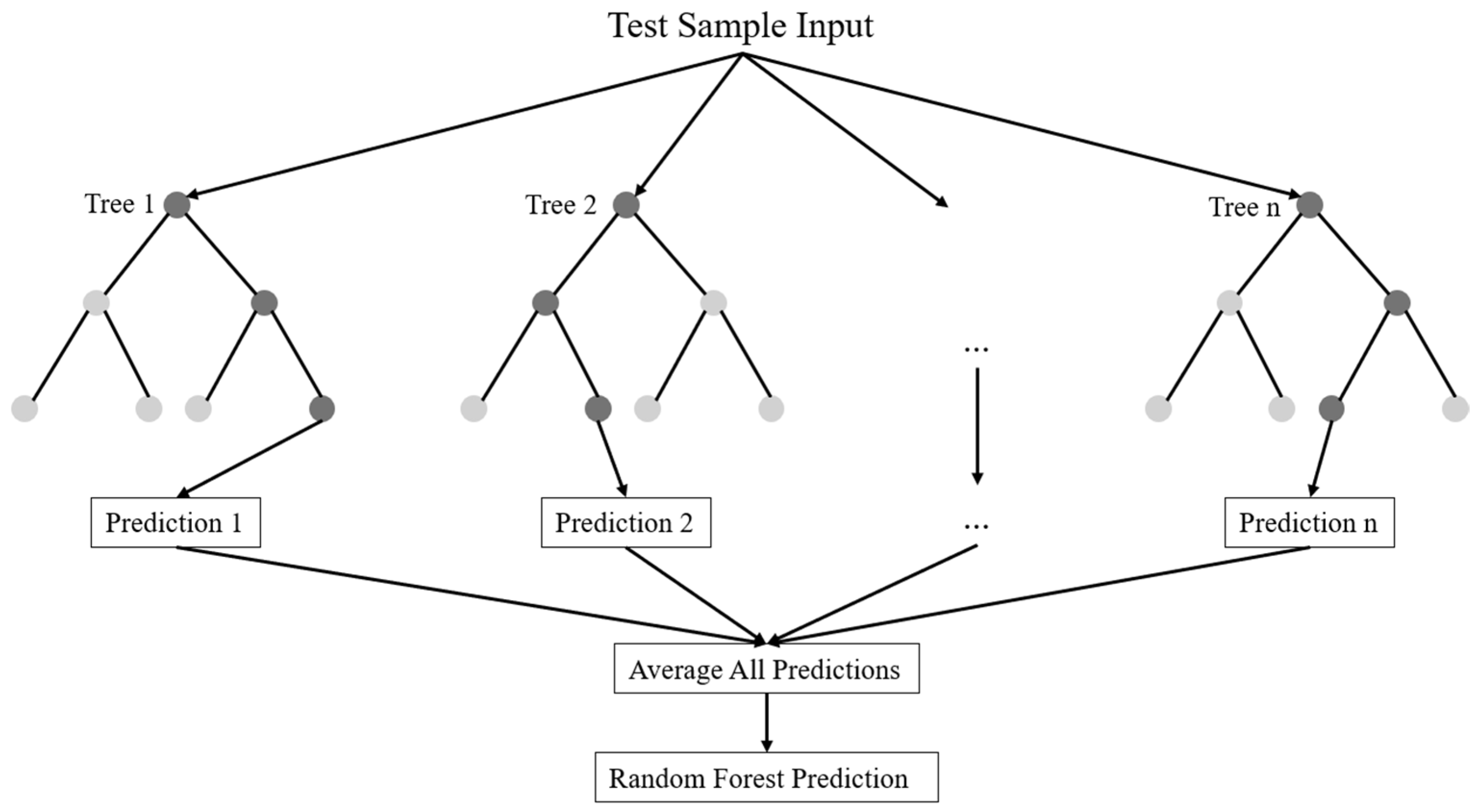
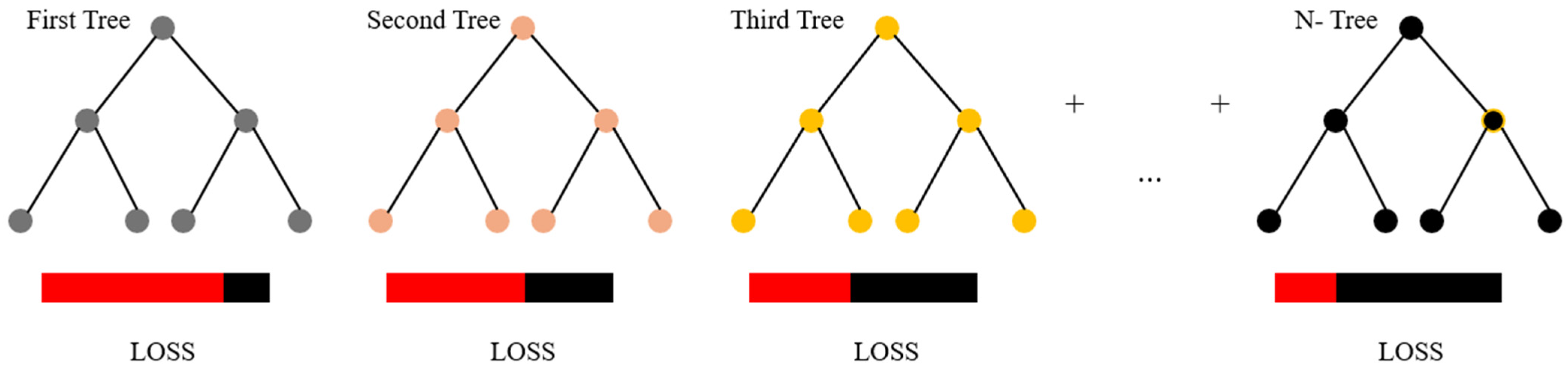
Damage to the wind turbine due to fatigue will cause economic damage and adversely affect energy production [23]. Therefore, accurate prediction of the fatigue life of wind turbine blades is of engineering importance. A review of the literature revealed that most of the studies did not use explainable ML models. In this study, random forest (RF), extreme gradient boosting (XGBoost), categorical boosting (CatBoost), light gradient boosting machine (LightGBM), and extra trees regressor (ExtraTrees) models are used to predict the fatigue life of the specimens. In order to establish the cause-and-effect relationship in the ML model, it is important to know which variables the model is based on. This is where explainable models come into the picture and give the most critical factors affecting the fatigue life of a turbine blade. For this reason, the SHapley Additive exPlanations (SHAP) approach was also used in this study to understand which variables the model is based on. Coefficient of determination (R²), mean squared error (MSE), and root mean squared error (RMSE) were chosen as performance metrics in this study.

2. Materials and Methods

2.1. Dataset

Materials subjected to repetitive or cyclic loads may be damaged over time under stresses that would not cause damage if applied once. This type of damage is referred to as fatigue damage. In order to evaluate the lifetime and durability of the material, it is important to examine the fatigue properties. Usually, S–N (Wöhler) curves (Figure 1) are used to determine these properties [24].

Although the Wöhler curve in Figure 1 is available for standard metals and alloys, such as aluminum alloys and steel, for more complex anisotropic or custom-made composite materials, these curves are not readily available. In composite materials and polymers, the curve has a negative slope, as the number of cycles in which damage occurs increases as the stress level decreases. In composite materials, the shape of the S–N curve varies depending on the type of matrix material, fiber orientation, volume fraction, interface properties, type of loading, average stress, average frequency, and environmental conditions [26]. In this study, the fiber volume fraction (Vf), percentages of the fiber orientation angle in the laminates (0°, 45°, and 90°), stacking sequence, fiber stress amplitude, loading frequency, laminate thickness, and the stress amplitude of a fatigue test carried out on a laminated composite specimen were used to predict the number of cycles, representing the fatigue life of the material. Thus, the aim was to develop a guiding and practical method in the design process by determining the inputs that will provide a longer fatigue life. It also enabled the comparison of different composite material configurations under different fiber volume fractions, fiber orientations, stacking sequences, laminate thicknesses, and stress amplitudes of fatigue or loading conditions, and can be effective when selecting the most suitable material and manufacturing method for a given application.

The dataset was taken from Hernandez-Sanchez et al. [27] and includes extensive measurements for fatigue life prediction for different loading conditions. The dataset was prepared in Excel for the analysis with machine learning models and had 8 inputs and 1 output and consisted of 855 rows in total. These data were generated from various fatigue tests. The inputs were fiber volume fraction (Vf), percentages of the fiber orientation angle in the laminates (0°, 45°, and 90°), stacking sequence, fiber stress amplitude, loading frequency, laminate thickness, and the stress amplitude of a fatigue test carried out on a laminated composite specimen. The output was the number of cycles, which indicated the fatigue life of a specimen. The variables in the dataset were statistically analyzed. First, a statistical summary of the dataset was made. Then, correlation analysis was performed to show the relationship between the variables and the direction and severity of this relationship. Then, separate graphs were created for the relationships between all inputs and the total number of cycles. The number of data points, mean, standard deviation, and minimum and maximum values of input and output variables in the dataset are given in

Table 1. Statistical summary of variables.

Variables	Count	Mean	Std.	Min.	Max.
Vf (%)	885	46.73	9.88	30.40	6350
0° (%)	885	61.58	29.74	0	100
45° (%)	885	33.80	27.41	0	99
90° (%)	885	4.29	8.53	0	25
Other (%)	885	0.31	1.35	0	8.30
Thickness (mm)	885	2.63	1.17	1.03	5.77
Frequency (Hz)	885	364.24	375.76	−41.40	2894
Total number of cycles	885	1.71	1.84	0.01	10

.

Fiber volume fraction refers to the percentage ratio of the fiber in the fiber-reinforced composite material to the total material volume [28]. The orientation of the fibers affects fatigue resistance, as the fibers increase the material’s resistance to cyclic loads and prolong fatigue life [29]. The orientations of the fibers used in this dataset were 0°, 45°, and 90°. Laminate thickness also influences fatigue life and, generally, the fatigue strength of the thinnest specimens is lower than that of other thicknesses [30]. Another significant input feature was the frequency of loading, which indicates the rate of load direction reversal between the highest values of stress and strain. The dataset also included specimens with fiber orientation angles other than 0°, 45°, and 90° (Figure 2). The volume fraction of these fiber orientations was included as an additional input feature. The output variable was the total number of cycles, which indicates the fatigue strength of the turbine blade.

A correlation matrix was created to examine the relationship between the variables (Figure 3). The correlation matrix showed that the highest relationship was between thickness and 90°. However, it was observed that no variable had a high correlation (>0.7) with the output variable.

Finally, the relationship between the input variables and the total number of cycles was visualized. Figure 4 shows the relationship between the input variables and the predicted fatigue life (total number of cycles). The data points represent experimental results obtained from different samples. From Figure 4, it is seen that the dependency of inputs with output was low. In general, it was observed that fatigue life varied greatly at low Vf, thickness, and high block max. stress input values. In other inputs, certain percentages of data points were clustered.

2.2. Machine Learning

The widespread use of technology in today’s world has led to a continuous increase in the amount of data generated by people. This increase has led to the creation of large datasets, enabling more data-driven decisions to be made in many sectors. Artificial intelligence (AI) enables meaningful insights from large datasets. AI is of great importance in many sectors today and in the future, and this importance is expected to increase. Machine learning (ML) is an AI approach that has the capacity to make predictions about future situations and make various inferences by performing statistical analysis on past data [31].

ML is widely used in civil engineering, such as in soil classification [32,33], maximum displacements of reinforced concrete (RC) beams under impact loading predictions [34], predicting the axial compression capacity of concrete-filled steel tubular columns [35], prediction of shear strength of rectangular RC columns [36], optimum design of reinforced concrete columns [37], prediction of basalt fiber-reinforced concrete splitting tensile strength [38], optimum design of welded beams [39], prediction of the debonding failure of beams strengthened with fiber-reinforced polymer [40], compressive strength prediction of ultra-high-performance concrete [41], reliability analysis of RC slab–column joints under punching shear load [42], cooling load prediction [43], shear wave velocity prediction [44], flexural capacity prediction of corroded RC beams, modeling of soil behavior [45], etc.

Figure 5 has been prepared to better depict the framework of the study.

The dataset was divided into training and test sets. Hyperparameter optimization was performed with GridSearchCV, and the results were evaluated with performance metrics. The models were interpreted using SHAP.

2.2.1. Random Forest

Random forest is a machine learning technique developed by Leo Breiman [46] in 2001. Since it can be used effectively for both classification and regression problems, it has become a flexible tool that can adapt to different types of problems. Random forest improves prediction accuracy by creating multiple decision trees in the regression process. Randomly selected decision trees come together to form a random forest model. The trees grow in the data learning process based on the complexity of the data [47]. Random forest reduces the correlation between decision trees and lowers variance by creating trees from different subsets of training data [46]. Random forest regression is shown in Figure 6.

2.2.2. Extreme Gradient Boosting (XGBoost)

XGBoost was introduced by Chen and Guestrin [49] in 2016 and is an ensemble learning method that aims to reduce model errors and make robust predictions by sequentially adding decision trees. This method is an optimized version of the gradient boosting algorithm and offers several improvements in terms of speed, performance, and accuracy. As an ensemble learning method, it aims to combine the predictions of multiple weak models to produce stronger and more successful predictions [49]. XGBoost starts by building a simple prediction model. At each iteration, the differences between the model’s current predictions and the actual values are calculated. These differences represent the information that needs to be learned in the next iteration. In each iteration, a new decision tree is added, which focuses on predicting the error terms of the previous model [50]. Figure 7 shows the XGBoost algorithm decision tree structure.

2.2.3. Categorical Boosting (CatBoost)

CatBoost is one of the next-generation versions of gradient boosting algorithms proposed by Prokhorenkova et al. [51] in 2018. This model is a powerful machine learning method designed to work effectively with categorical features and to achieve high performance by quantifying categorical data [51]. CatBoost aims to minimize information loss while working with categorical and numerical data. CatBoost has advantages of high learning speed, visualization capabilities, and the ability to work effectively with both categorical and numerical data. Figure 8 shows the CatBoost regression algorithm [52].

2.2.4. Light Gradient Boosting Machine (LightGBM)

LightGBM is a machine learning algorithm developed by Ke et al. [53] in 2017 based on decision trees and boosting algorithms, designed to improve existing boosting methods. Its most notable difference from existing boosting methods is its efficiency and lightweight nature, which speeds up the training process. LightGBM offers high performance and fast learning, especially on large datasets [54]. One of the key features that distinguishes LightGBM from other tree augmentation algorithms is that it splits the tree in the direction of the leaf to achieve the best fit (Figure 9). This approach allows it to learn with less loss compared to algorithms that split by level when growing the same leaf [55].

2.2.5. Extremely Randomized Trees Regressor (ExtraTrees Regressor)

The ExtraTrees regressor method developed by Geurts et al. [57] in 2006 uses different samples of the dataset in the training phase, as in the random forest model. However, instead of using decision trees for optimal separation of nodes into branches, a random partitioning method is preferred. While this approach reduces the computational burden and complexity of the model in data analysis problems, it can lead to poor performance on large datasets [58]. The ExtraTrees algorithm is similar in performance to other tree-based algorithms but has a higher computational speed [57]. Figure 10 shows the ExtraTrees regression [53].

2.3. Principal Component Analysis (PCA)

Principal component analysis (PCA) was developed by Pearson [60] in 1901 and then independently of Pearson by Hotelling [61] in 1930. PCA is a multivariate technique that examines correlations between observations and analyzes multiple quantitative dependent variables. PCA is a method for dimension reduction without any loss of essential information in the original dataset. The most popular statistical analysis method used to select the appropriate dataset as input for modeling is PCA [62]. In factor analysis, PCA is the most common multivariate statistical technique used to reduce many interrelated variables into fewer, significant, and independent factors [63]. Figure 11 shows the PCA flowchart [64].

When PCA is approached from the perspective of maximizing variance, the goal is to project the M N-dimensional vectors that make up the dataset into an m-dimensional subspace in a way that maximizes the variance of their projections [65].

2.4. Hyperparameter Optimization

Hyperparameter optimization is a method to improve the performance of ML models. Hyperparameters are critical elements that directly affect the learning process and the overall behavior of the model. The main objective of hyperparameter optimization is to determine the combination of hyperparameters that maximizes the performance of the model. Correctly chosen hyperparameters can enable the model to generalize better, prevent problems, such as overlearning and underlearning, and accelerate the learning process. In this study, the GridSearchCV method was used to determine the optimal parameters for the models [66].

GridSearchCV is a method that tries all possible combinations to identify the best hyperparameters. First, different values are set for each hyperparameter and all possible combinations of them are generated. Then, the model is trained using each combination, and its performance is measured by cross-validation. The hyperparameter combination that gives the best performance is selected, and the model is run with these settings. However, as the number of hyperparameters increases, the number of combinations to be tried increases rapidly. With a large number of hyperparameters and a wide range of values, the computational cost can be high [67,68]. Figure 12 shows the hyperparameter optimization using GridSearhCV.

2.5. Training–Test Split

The data to be used in the analysis were divided as 80% training data and 20% test data (Figure 13). The 20%–80% split was chosen because it is a commonly used ratio in the literature [70]. The model was split in two to use different data to train the model and to measure the overall performance of the model. The training set was used to learn the model, while the test set was used to measure the real-life performance of the model. It is necessary to test the model with data that the model has not seen before, data that were not used in the training and validation phases. This dataset was used to evaluate the generalization ability of the model.

2.6. Performance Metrics in Machine Learning Methods

Performance metrics are used to assess how effectively a model works. The performance metrics (coefficient of correlation (R²), mean squared error (MSE), and root mean squared error (RMSE)) used in this study are explained below.

2.6.1. Coefficient of Correlation (R²)

The coefficient of correlation (R²) reflects the strength and direction of the linear relationship between predicted and actual values. A value close to 1 indicates a strong positive correlation, while values close to 0 indicate weak or no correlation [71]:

$${\mathrm{R}}^2=1-{\displaystyle \frac{{\sum }_{\mathrm{i}=1}^{\mathrm{N}}{({\mathrm{y}}_{\mathrm{a}\mathrm{c}\mathrm{t}\mathrm{u}\mathrm{a}\mathrm{l}}-{\mathrm{y}}_{\mathrm{p}\mathrm{r}\mathrm{e}\mathrm{d}})}^2}{{\sum }_{\mathrm{i}=1}^{\mathrm{N}}{\left({\mathrm{y}}_{\mathrm{a}\mathrm{c}\mathrm{t}\mathrm{u}\mathrm{a}\mathrm{l}}\right)}^2}}$$

(1)

2.6.2. Mean Squared Error (MSE)

Mean squared error (MSE) evaluates the mean square difference between observed and predicted values. When there is no error in a model, the MSE is equal to zero. Its value increases as the model error increases [72]:

$$\mathrm{M}\mathrm{S}\mathrm{E}={\displaystyle \frac{1}{\mathrm{N}}}{\sum }_{\mathrm{i}=1}^{\mathrm{N}}{({\mathrm{y}}_{\mathrm{a}\mathrm{c}\mathrm{t}\mathrm{u}\mathrm{a}\mathrm{l}}-{\mathrm{y}}_{\mathrm{p}\mathrm{r}\mathrm{e}\mathrm{d}})}^2$$

(2)

2.6.3. Root Mean Squared Error (RMSE)

Root mean squared error (RMSE) measures the average difference between the predicted values of the statistical model and the actual values. Mathematically, it is the standard deviation of the residuals. The RMSE is calculated by taking the square root of the MSE [73]:

$$\mathrm{R}\mathrm{M}\mathrm{S}\mathrm{E}=\sqrt{{\displaystyle \frac{1}{\mathrm{N}}}{\sum }_{\mathrm{i}=1}^{\mathrm{N}}{({\mathrm{y}}_{\mathrm{a}\mathrm{c}\mathrm{t}\mathrm{u}\mathrm{a}\mathrm{l}}-{\mathrm{y}}_{\mathrm{p}\mathrm{r}\mathrm{e}\mathrm{d}})}^2}$$

(3)

2.7. SHapley Additive exPlanations (SHAP)

SHAP is a method developed by Lundberg and Lee [74] in 2017 to improve the interpretability of individual forecasts. This method allows to explain the decision mechanism of the model by calculating the contribution of each feature to the prediction. SHAP evaluates all possible combinations of attributes based on Shapley values in game theory and thus provides consistent and interpretable explanations at both local and global scales. SHAP analysis helps to identify redundant variables by showing, through graphs, which features are important in the model. Shapley values with larger absolute values indicate that the feature has a greater influence on the prediction [74].

The study utilized a system with an Intel(R) Core (TM) i3-7000 CPU @ 3.90 GHz processor, 768 GB system memory, and 24 GB video card.

3. Results and Discussion

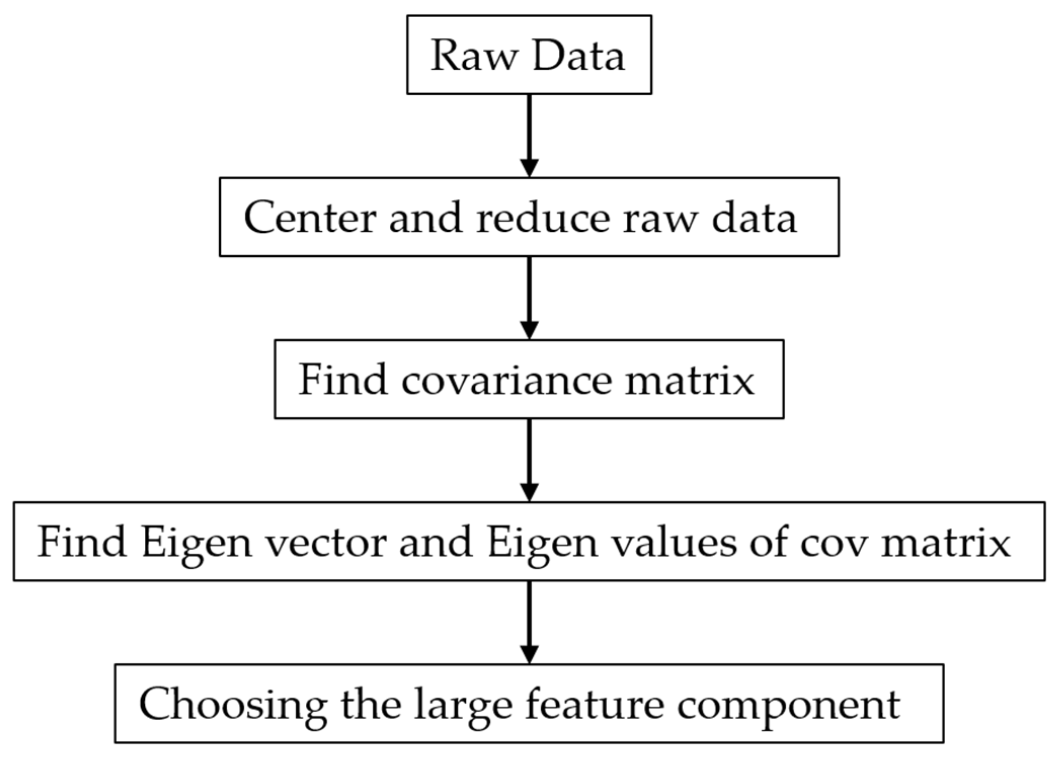
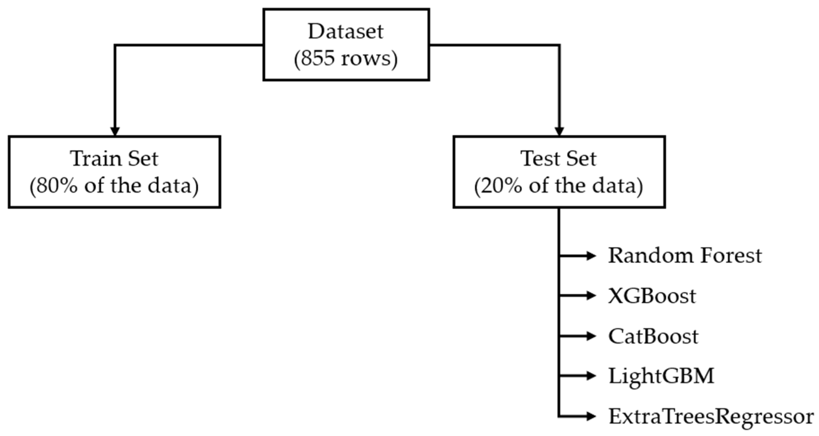
In this study, the number of cycles, which indicates the fatigue life of a specimen, was estimated by using random forest (RF), extreme gradient boosting (XGBoost), categorical boosting (CatBoost), light gradient boosting machine (LightGBM), and ExtraTrees regressor algorithms from ML methods. Coefficient of correlation (R²), mean squared error (MSE), and root mean squared error (RMSE) values for the dataset were calculated to measure the accuracy of the predictions. SHAP analysis was then performed. The results obtained from the machine learning algorithms applied to the dataset were as follows: ML models analyzed on the fatigue dataset were optimized with principal component analysis (PCA).

Coefficient of correlation (R²), mean squared error (MSE), and root mean squared error (RMSE) were used to evaluate the performance of the models. These metrics were used as benchmarks for the predictions performed on the training and test sets.

Table 2. Random forest results in PCA optimization and hyperparameter optimization.

Metrics	Training Set	Test Set
R2	0.9670	0.9052
RMSE	0.8543	1.3683
MSE	0.7299	1.8724

gives the metrics of the training and test sets using random forest. In the training set, the model showed an R² of 0.9670, RMSE of 0.8543, and MSE of 0.7299. However, in the test set, the R² decreased to 0.9052, and the error values increased (MSE = 1.3683 and RMSE = 1.8724). This indicates that the model performed well on the test set and was not overfitting but did not generalize as well as on the training set. Since hyperparameter optimization was performed using GridSearchCV, it can be said that this was due to the nature of the data. The best hyperparameters for random forest were {‘max_depth’: 10, ‘min_samples_leaf’: 1, ‘min_samples_split’: 2, ‘n_estimators’: 200}.

Table 3. XGBoost results in PCA optimization and hyperparameter optimization.

Metrics	Training Set	Test Set
R2	0.9548	0.8958
RMSE	1.00005	1.4346
MSE	1.00011	2.0582

gives the metrics of the training and test sets using XGBoost. In the training set, the model showed an R² of 0.9548, RMSE of 1.00005, and MSE of 1.00011. However, in the test set, the R² decreased to 0.8958, and the error values increased (MSE = 1.4346 and RMSE = 2.0582). This indicates that the model performed well on the test set and was not overfitting but did not generalize as well as on the training set. Since hyperparameter optimization was performed using GridSearchCV, it can be said that this was due to the nature of the data. The best hyperparameters for XGBoost were {‘colsample_bytree’: 1.0, ‘learning_rate’: 0.1, ‘max_depth’: 3, ‘n_estimators’: 200, ‘subsample’: 0.8}.

Table 4. CatBoost results in PCA optimization and hyperparameter optimization.

Metrics	Training Set	Test Set
R2	0.9468	0.9027
RMSE	1.0850	1.3862
MSE	1.1772	1.9215

gives the metrics of the training and test sets using CatBoost. In the training set, the model showed an R² of 0.9468, RMSE of 1.0850, and MSE of 1.1772. However, in the test set, the R² decreased to 0.9027, and the error values increased (MSE = 1.3862 and RMSE = 1.9215). This indicates that the model performed well on the test set and was not overfitting but did not generalize as well as on the training set. Since hyperparameter optimization was performed using GridSearchCV, it can be said that this was due to the nature of the data. The best hyperparameters for CatBoost were {‘bagging_temperature’: 0.0, ‘depth’: 8, ‘iterations’: 50, ‘l2_leaf_reg’: 1, ‘learning_rate’: 0.2}.

Table 5. LightGBM results in PCA optimization and hyperparameter optimization.

Metrics	Training Set	Test Set
R2	0.9658	0.9054
RMSE	0.8701	1.3668
MSE	0.7571	1.8682

gives the metrics of the training and test sets using LightGBM. In the training set, the model showed an R² of 0.9658, RMSE of 0.8701, and MSE of 0.7571. However, in the test set, the R² decreased to 0.9054, and the error values increased (MSE = 1.3668 and RMSE = 1.8682). This indicates that the model performed well on the test set and was not overfitting but did not generalize as well as on the training set. Since hyperparameter optimization was performed using GridSearchCV, it can be said that this was due to the nature of the data. The best hyperparameters for LightGBM were {‘learning_rate’: 0.1, ‘max_depth’: 4, ‘n_estimators’: 200, ‘num_leaves’: 31, ‘reg_alpha’: 0.1, ‘reg_lambda’: 1.0}.

Table 6. ExtraTrees regressor results with PCA optimization and hyperparameter optimization.

Metrics	Training Set	Test Set
R2	0.9154	0.8958
RMSE	1.3683	1.4344
MSE	1.8724	2.0576

gives the metrics of the training and test sets using ExtraTrees regressor. In the training set, the model showed an R² of 0.9154, RMSE of 1.3683, and MSE of 1.8724. However, in the test set, the R² decreased to 0.8958, and the error values increased (MSE = 1.4344 and RMSE = 2.0576). This indicates that the model performed well on the test set and was not overfitting but did not generalize as well as on the training set. Since hyperparameter optimization was performed using GridSearchCV, the very small difference between the test and training metrics suggests that the model was not overfitting but that some caution should be exercised against some uncertainty in the test data. This was due to the nature of the dataset. The best hyperparameters for ExtraTrees regressor were {‘max_depth’: 8, ‘min_samples_leaf’: 1, ‘min_samples_split’: 2, ‘n_estimators’: 200}.

GridSearchCV was used to avoid the risk of overfitting, and the biggest difference between training and test performance (about 0.06) in Table 2, Table 3, and Table 5 was acceptable.

In the analyses performed with the dataset, prediction was made with five different algorithms, and the performances of all models are given in

Table 7. Performance comparison of all algorithms used in this study for the test set.

Metrics	R2	RMSE	MSE
Random Forest	0.9052	1.3683	1.8724
XGBoost	0.8958	1.4346	2.0582
CatBoost	0.9027	1.3862	1.9215
LightGBM	0.9054	1.3668	1.8682
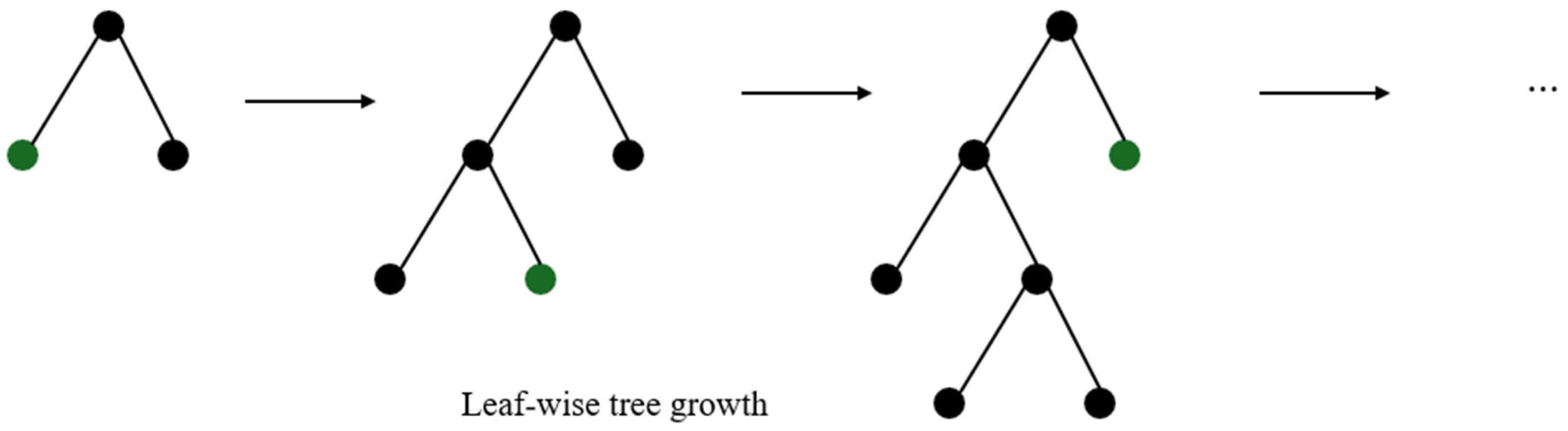
ExtraTrees Regressor	0.8958	1.4344	2.0576

. Using three different metrics, the results were satisfactory. The most successful algorithm was the category boosting LightGBM, with an R² of 0.9054, RMSE of 1.3668, and MSE of 1.8682. Unlike other methods, LightGBM may have shown the highest performance because it splits the tree in the direction of the leaf to obtain the best fit, uses histogram-based optimization, and is more efficient and lightweight. The other two best algorithms were random forest and CatBoost.

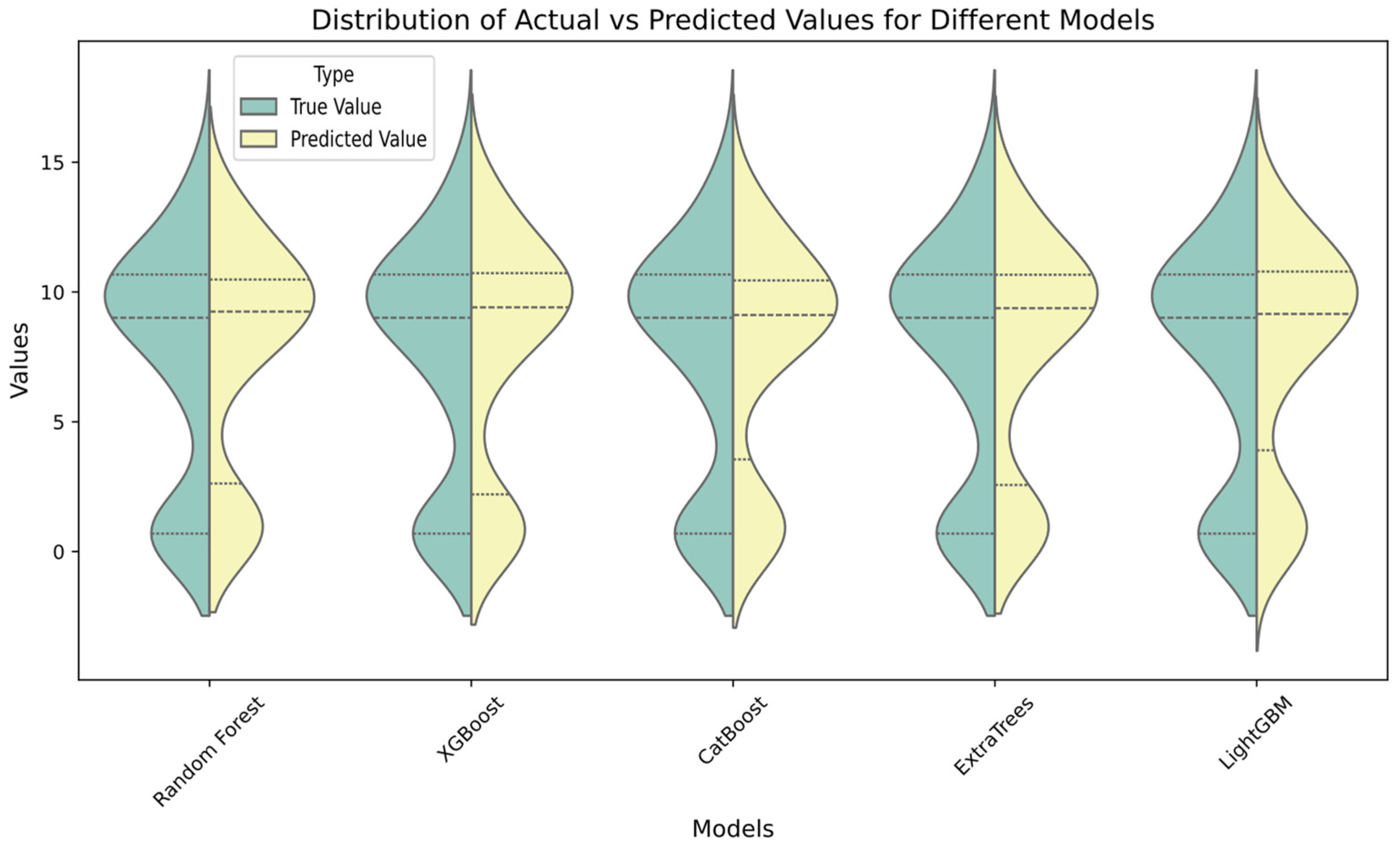
These results in Table 7 show that decision-tree-based models showed a strong predictive ability on the dataset. Figure 14 gives the violin plots for error distributions (true–predicted) for the models used in this study. In Figure 14, the violin plot is used to visualize the prediction performance of different ML models used in this study. The X-axis shows the ML models used in the study, and the Y-axis shows the distribution of actual and predicted values. Green is the distribution of true values and yellow is the distribution of model-predicted values.

In Figure 14, the line in the middle of each ML model shows the average of the actual or predicted values. Using the violin plot, the distribution and probability density of the data can be evaluated by looking at the visuals. It is seen that the predicted and observation values were close to each other in the ML models.

Figure 15 shows the scatter plots of the ML models used in the study. Using these plots, the relationship between the actual values and the values predicted by the models can be understood. In the graphs, which can be viewed as data point distributions, it is seen that these distributions were more homogeneous in random forest and LightGBM than in the other models in Figure 15. However, the point distribution was good in the other models as well. Even though the data were randomly distributed, it was at an acceptable level.

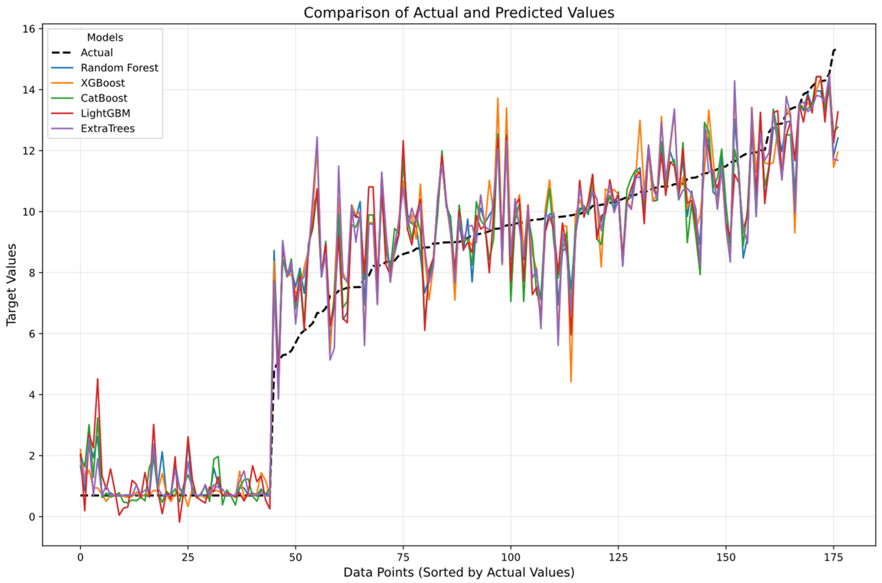
Figure 16 shows the line plot of the ML models used in the study. A comparison of actual and predicted values can be done using this plot. Random forest and LightGBM were closer to the actual values than the other models, as shown in Figure 16. The jump in the curve (at the 45th point) was due to the differences in the fatigue resistance of different specimens. Also, the values in Figure 16 are the transformed values as a result of PCA.

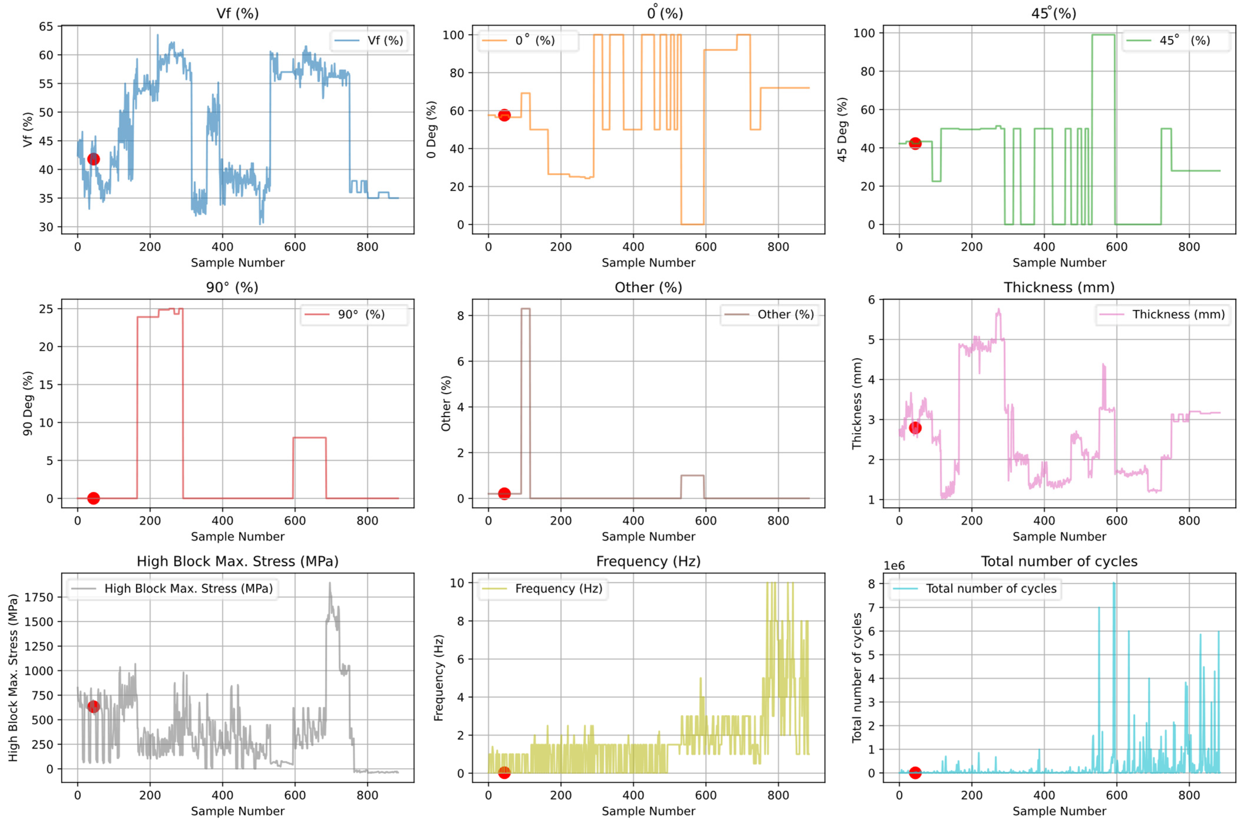
Each variable in the real dataset is shown as a line plot in Figure 17, with data point 45 highlighted in red for clarity. Using the actual values, there was no jump at data point 45.

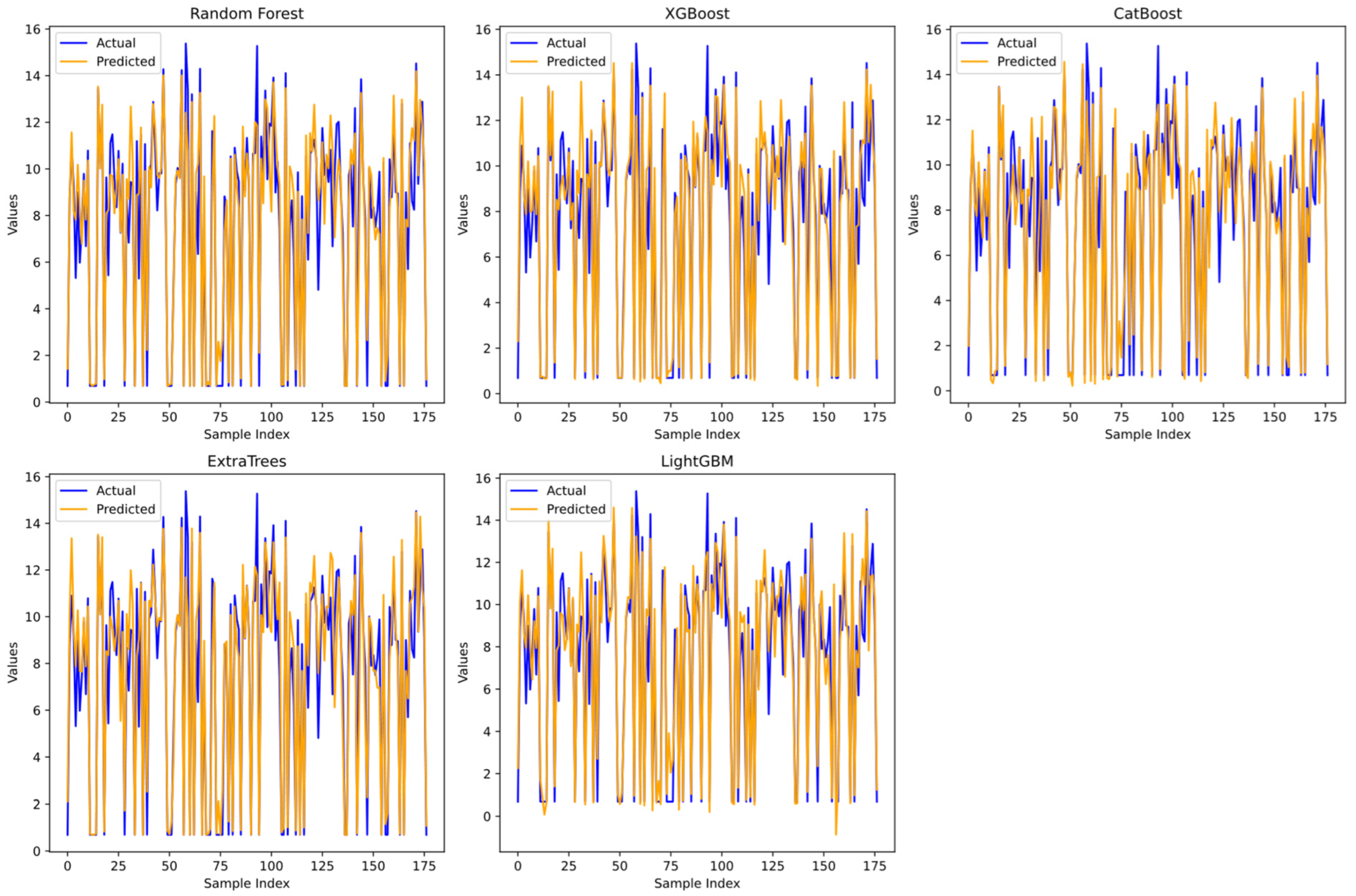
In addition, individual line plots for all ML models are shown in Figure 18. Figure 18 shows a comparison of the values predicted by ML models and the actual values. The blue line represents the actual values, and the orange line represents the predicted values. Although there were significant deviations in some examples, in general, the orange line (predicted) and the blue line (actual) were quite close to each other at most points, indicating that the models were able to make predictions close to the actual values.

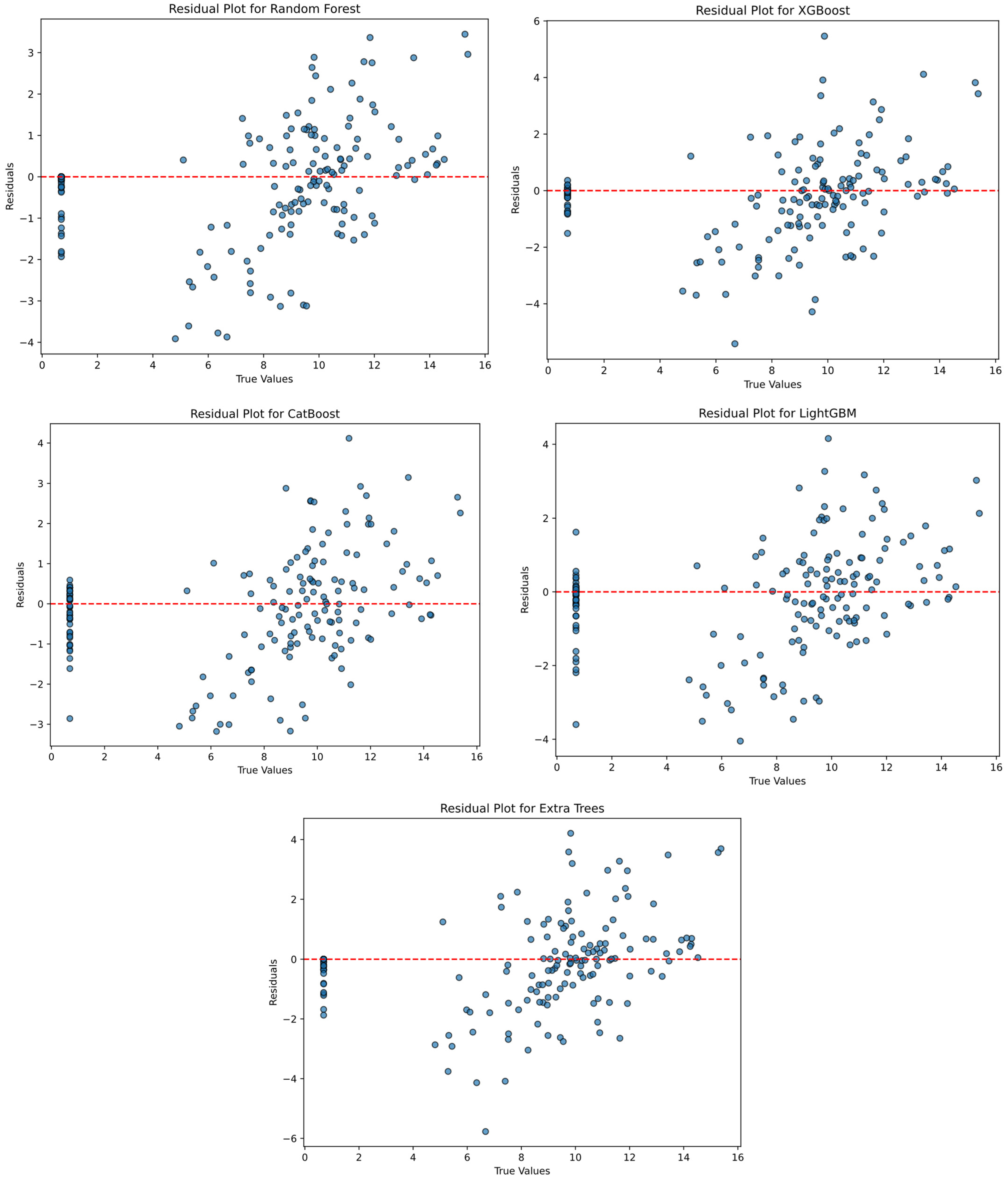
Figure 19 presents residual plots for random forest, XGBoost, CatBoost, LightGBM, and ExtraTrees. The X-axis represents the true values, and the Y-axis represents the residuals. The red dashed line represents the baseline where residual values should be evenly distributed around zero. Although the residual values were generally distributed around the red dashed line, as expected, in certain ranges, deviations were observed.

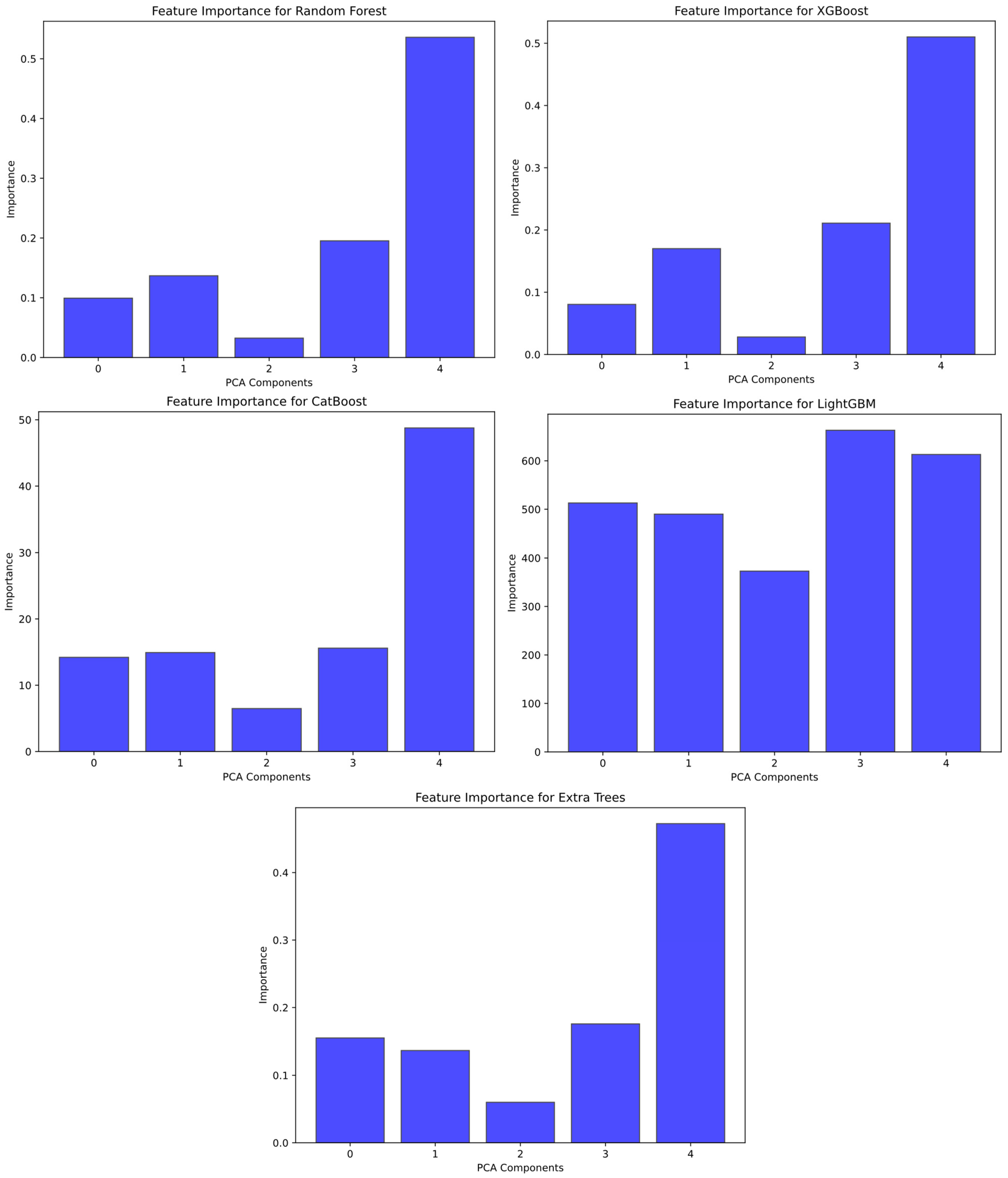
As seen in Figure 19, the random distribution of points in the residual plots indicated that the models predicted the data well. Since the residuals were randomly distributed around zero, the models showed good performance. Figure 20 presents feature importance plots for random forest, XGBoost, CatBoost, LightGBM, and ExtraTrees. Figure 20 shows the PCA components (1, 2, …, n) on the X-axis and the feature contribution of the model on the Y-axis. In general, the fifth component had the highest score, so the greatest variability of the data may be captured in the fifth component.

Feature importance is a measure of which features have more influence in a model. For example, according to the feature importance and PCA results obtained from the LighgtGBM model, features 3 and 4 had the highest scores and contributed significantly to the model’s predictions. This indicates that the model took these two features into account more when making accurate predictions. This suggests that the model can work with a lower dimensional representation and simplify the data without losing significant information. A 100% variance rate was achieved in component 8.

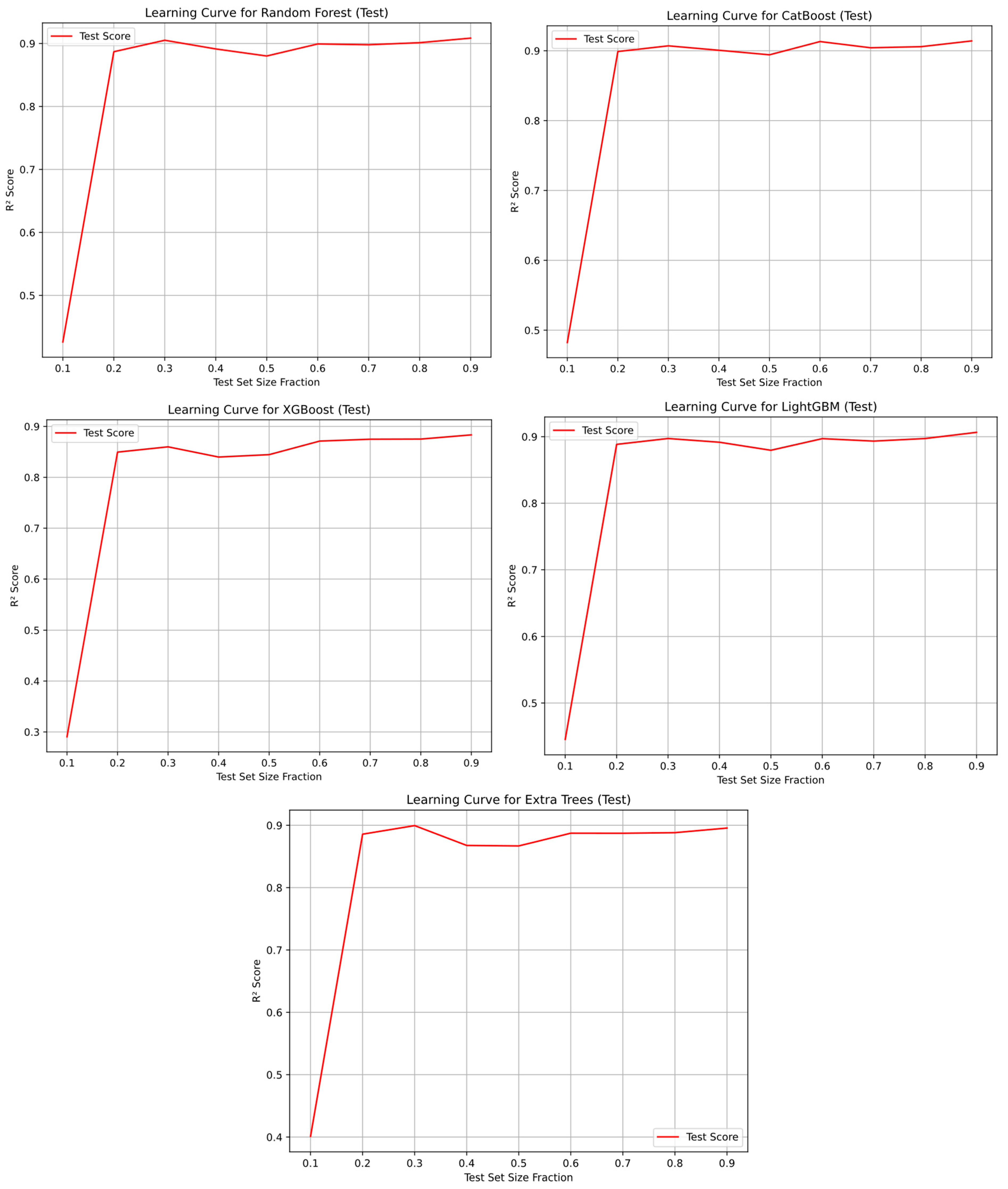
The learning curve is a graph that visualizes the change in performance of a model during the training process. This curve provides information about the model’s learning process on training data and how much it generalizes on test data. Figure 21 shows learning curves for random forest, XGBoost, CatBoost, LightGBM, and ExtraTrees.

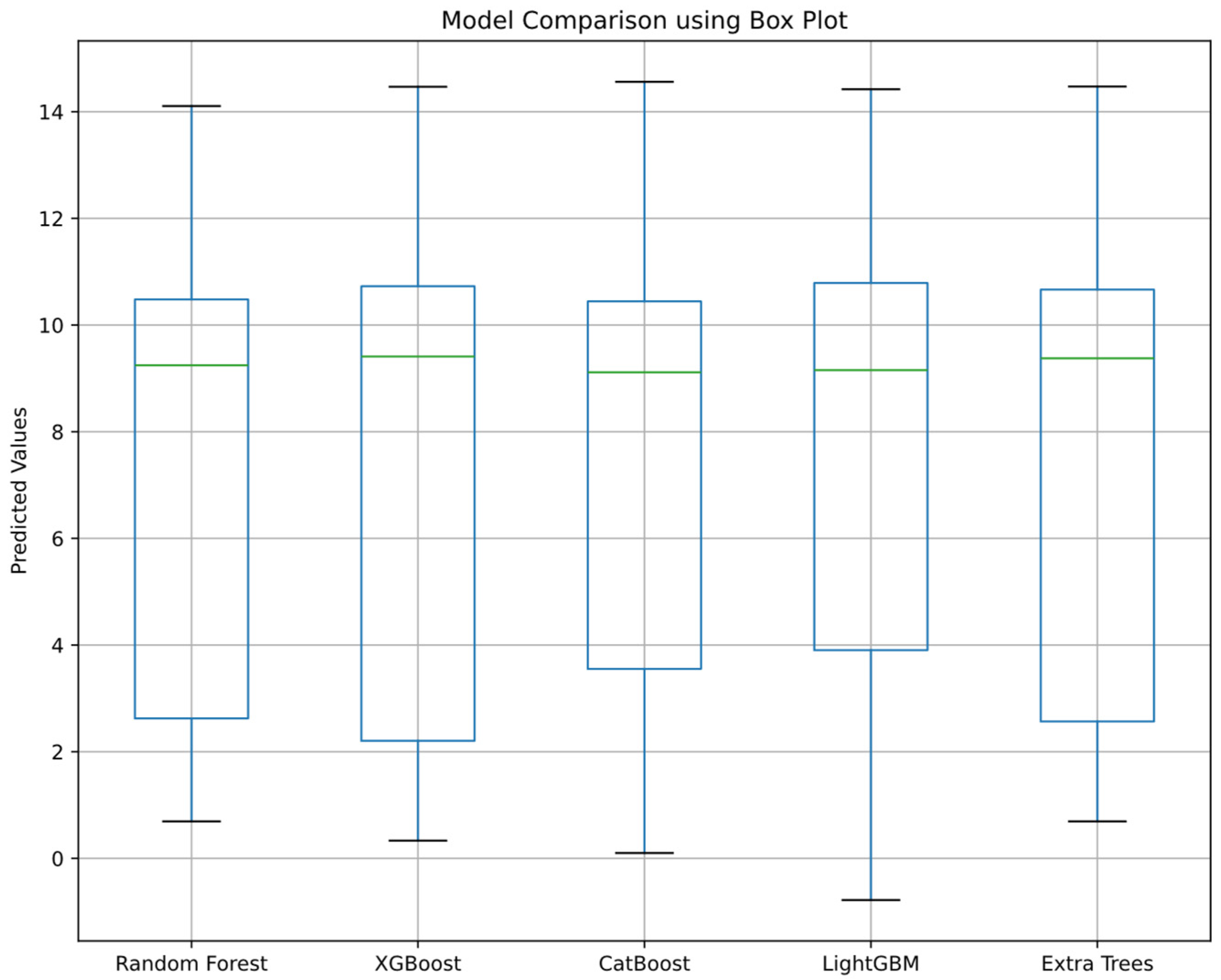
As seen in Figure 21, there was an increase in the test R² value in the learning curve graphs. Figure 22 compares the prediction performance of random forest, XGBoost, CatBoost, LightGBM, and ExtraTrees using a box plot. On the X-axis are the machine learning models, and on the Y-axis are the predicted values. The box plots show the prediction distribution and central tendency of each model.

According to the box plot results in Figure 22, it is clear from the box widths that LightGBM, random forest, and CatBoost performed better than the other models. Using the LightGBM algorithm, which was the most successful of all the algorithms, a SHAP bar plot was drawn, and it was observed which variable had the most impact on the predictions. In the LightGBM model, the SHAP method was used to visually explain how inputs affected the number of cycles, which indicates the fatigue life of a specimen. 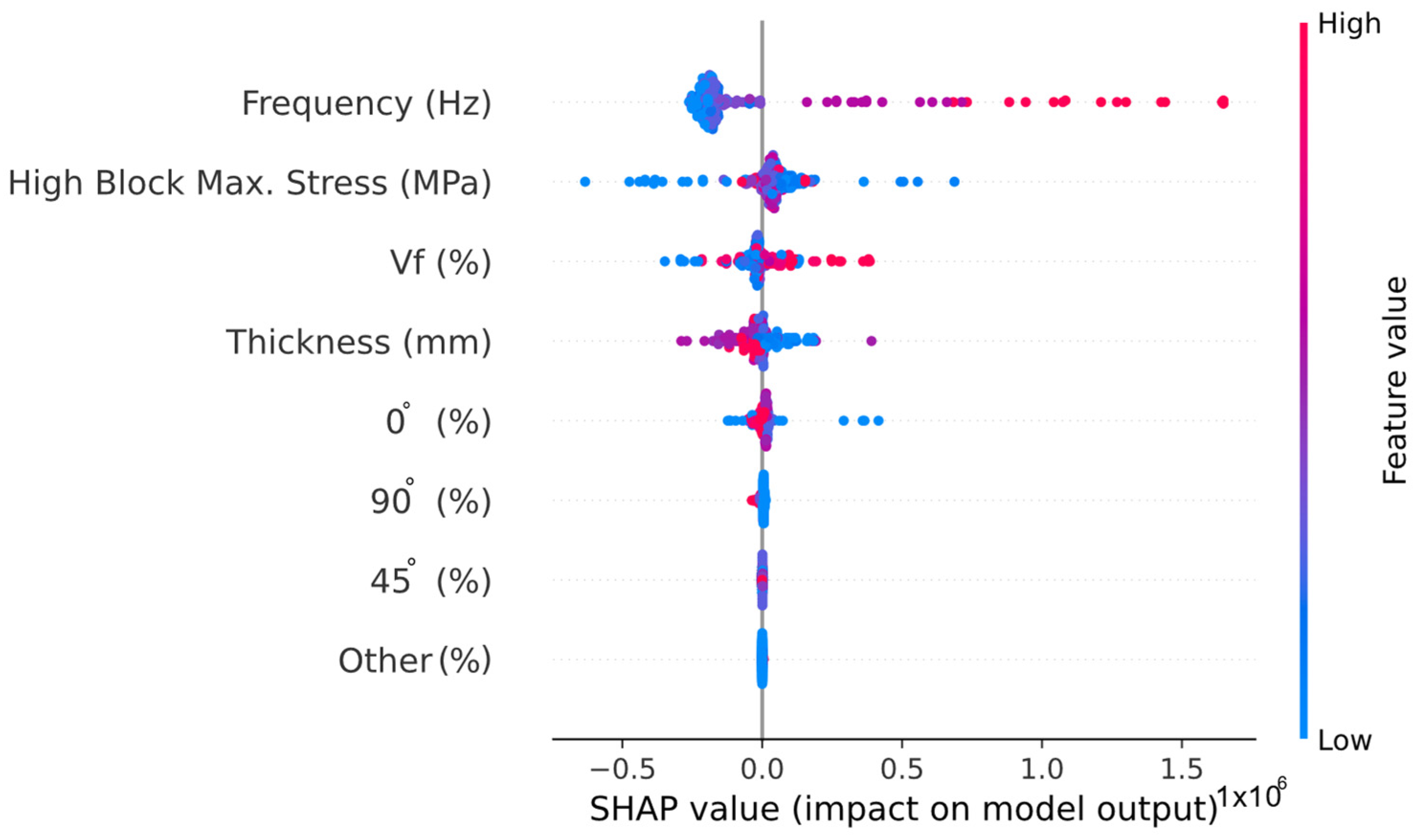Figure 23 shows the importance rankings of the variables obtained as a result of SHAP analysis using the LightGBM algorithm.

As can be seen from Figure 23, the variable that affected the number of cycles, which indicates the fatigue life of a specimen, the most was frequency. High block max. stress, Vf, and thickness came after frequency. Therefore, it can be said that these four inputs had the biggest impact on output. Figure 24 shows the SHAP decision plot using LightGBM. This plot shows which inputs were most influential in the decision process.

As shown in Figure 24, it can be said that frequency, Vf, thickness, and high block max. stress inputs had the biggest impact on output.

In this study, tree-based ML methods were preferred due to their shorter training time and lower computational resource requirements. In contrast, deep learning (DL) models were not used due to their long training time and high hardware requirements. Furthermore, since explainability is an important factor in this study, tree-based ML methods, which are more interpretable, were chosen instead of DL models.

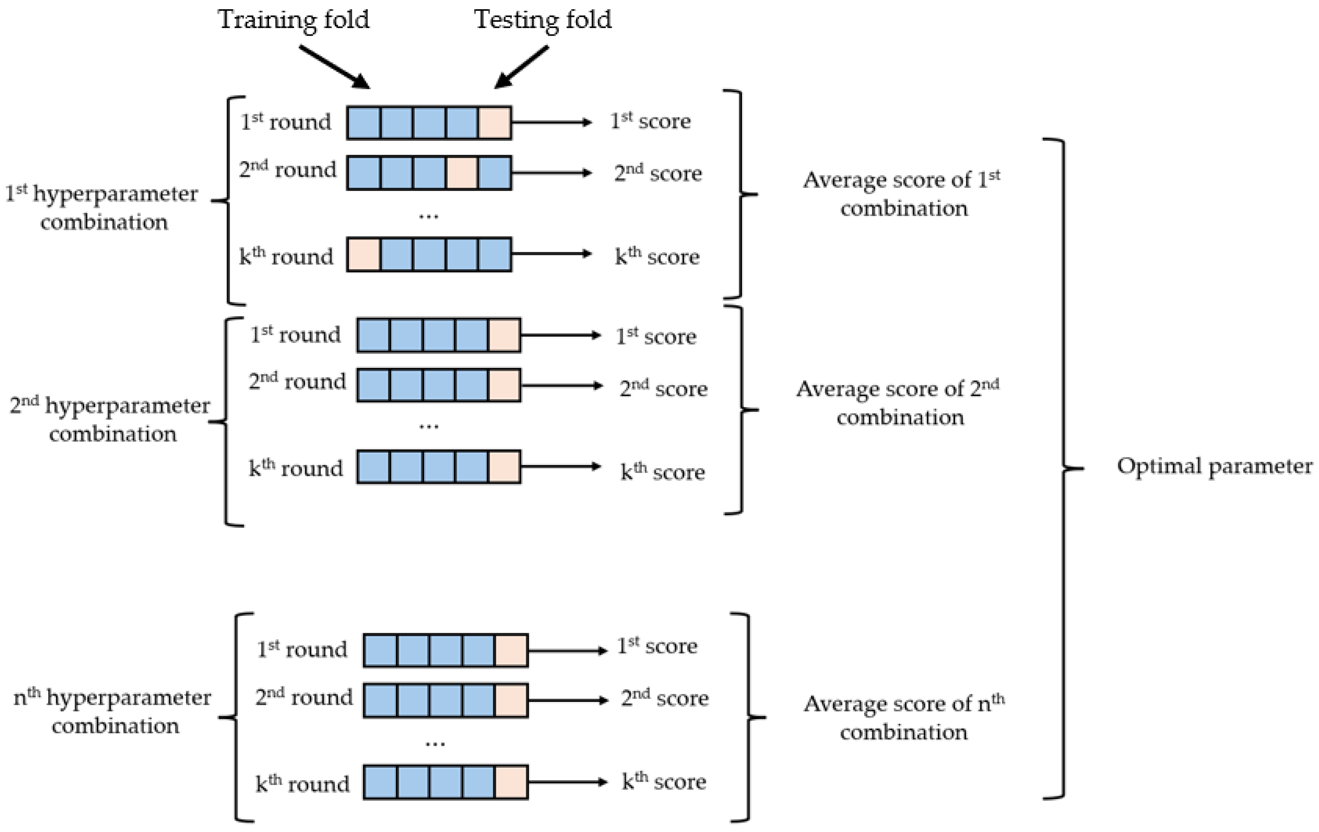
Hyperparameter optimization was performed using the GridSearchCV optimization method in this study. Thus, it offered a rigorous search process for the best performance of the model. GridSearchCV evaluates the model on different subsets of data to determine the most appropriate hyperparameter values and tries all possible combinations to identify the best hyperparameters. However, increasing the number of parameters increases the computation time. For this reason, the range of parameters for hyperparameter optimization was limited in the analysis code to optimize the performance of the model. Thus, the aim was both to improve the performance of the model and to keep the computational time of the optimization process at a reasonable level.

In the existing studies in the literature, it has been observed that the use of ANN is widespread for the fatigue life of wind turbine blades. For example, Ziane et al. [22] used the back propagation neural network (BPNN), particle swarm optimization-based artificial neural network (PSO-ANN), and cuckoo search (CS)-based NN to predict the wind turbine blade fatigue life under varying hygrothermal conditions and achieved up to 94% accuracy. In this study, a dataset with inputs, such as different fiber ratios and orientation angles, was used to predict the fatigue life of wind turbine blades, and training set R² values of up to 96% and test set R² values of up to 90% were achieved using ML models.

In order to reduce the risk of overfitting the model, cross-validation was performed on the dataset to analyze how the model performed on different data subsets. Furthermore, SHAP plots were plotted using LightGBM to examine the effect of each parameter on fatigue life prediction. These graphs showed that frequency was the most effective parameter in fatigue life prediction.

The current study proposed a data-driven approach to predict the fatigue life of laminated composite wind turbine blades with varying stacking sequence configurations. The analyzed dataset also included fiber orientations outside the commonly used ±45°, 90°, and 0° orientations. Since there are no closed-form predictive equations available for predicting the fatigue life of composite materials with randomly oriented fibers, the best approach would be to use data-driven techniques. The accuracy and reliability of these techniques can be verified using statistical metrics of accuracy. A limitation of the current study was the size of the dataset and the value ranges of the input features, which can be enhanced in future studies as more data become available.

4. Conclusions

Predicting the fatigue life of composite materials for wind turbine blades is a critical factor for wind turbines. With more accurate prediction methods, the lifetime of the wind turbine can be extended. In this study, the best low-error prediction algorithm was investigated using the dataset from the existing study. Five different algorithms were used: random forest (RF), extreme gradient boosting (XGBoost), categorical boosting (CatBoost), light gradient boosting machine (LightGBM), and ExtraTrees regressor.

The dataset was taken from Hernandez-Sanchez et al. [27]. The dataset had 885 rows, 8 inputs, and 1 output. In the study, after examining and cleaning the dataset, PCA and hyperparameter optimization using GridSearchCV were performed. The number of cycles, which indicates the fatigue life of a specimen, was predicted using the stacking sequence, fiber volume fraction, stress amplitude, loading frequency, laminate thickness, and the number of cycles of a fatigue test carried out on a laminated composite specimen using the five different ML algorithms. These algorithms were compared using the coefficient of correlation (R²), mean squared error (MSE), and root mean squared error (RMSE) to evaluate the performance of the models. In this comparison, it was concluded that the best method for predicting the fatigue life of composite materials for wind turbine blades was LightGBM. The importance levels of the variables were analyzed using SHAP, and it was seen that frequency was the most important factor that significantly affected the fatigue life of composite materials for wind turbine blades’ prediction. The obtained results showed that machine learning methods are promising in fatigue life prediction of composite materials for wind turbine blades. As a result of the study, the prediction values were found to be close to the real values.

Future studies could enhance the results by incorporating additional variables, employing different AI models, or gathering data from diverse locations. If these machine learning methods are used, it would be possible to make predictions at different operating intervals and with a new dataset. Other test split ratios, such as 30%–70%, 40%–60%, or 50%–50%, could also be tested on ML models. Future work could also consider the provisions of the ISO guidelines for condition monitoring and diagnostics of machines.

References

1. Jaiswal, K.K.; Chowdhury, C.R.; Yadav, D.; Verma, R.; Dutta, S.; Jaiswal, K.S.; Karuppasamy, K.S.K. Renewable and sustainable clean energy development and impact on social, economic, and environmental health. Energy Nexus 2022, 7, 100118. [Google Scholar] [CrossRef]
2. IRENA (2024)–Processed by Our World in Data. Installed Wind Energy Capacity. 2024. Available online: https://ourworldindata.org/grapher/cumulative-installed-wind-energy-capacity-gigawatts?country=~OWID_WRL (accessed on 22 January 2025).
3. Chaudhuri, A.; Datta, R.; Kumar, M.P.; Davim, J.P.; Pramanik, S. Energy Conversion Strategies for Wind Energy System: Electrical, Mechanical and Material Aspects. Materials 2022, 15, 1232. [Google Scholar] [CrossRef] [PubMed]
4. Patil, N.A.; Arvikar, S.A.; Shahane, O.S.; Rajasekharan, S.G. Estimation of dynamic characteristics of a wind turbine blade. Mater. Today Proc. 2022, 72, 340–349. [Google Scholar] [CrossRef]
5. World Wild Life. The Energy Report. Available online: https://www.worldwildlife.org/publications/the-energy-report (accessed on 23 January 2025).
6. Sayed, E.T.; Wilberforce, T.; Elsaid, K.; Rabaia, M.K.H.; Abdelkareem, M.A.; Chae, K.-J.; Olabi, A. A critical review on environmental impacts of renewable energy systems and mitigation strategies: Wind, hydro, biomass and geothermal. Sci. Total Environ. 2021, 766, 144505. [Google Scholar] [CrossRef]
7. Machado, M.; Dutkiewicz, M. Wind turbine vibration management: An integrated analysis of existing solutions, products, and Open-source developments. Energy Rep. 2024, 11, 3756–3791. [Google Scholar] [CrossRef]
8. Burton, T.; Jenkins, N.; Sharpe, D.; Bossanyi, E. Wind Energy Handbook; John Wiley & Sons Ltd.: Chichester, UK, 2011. [Google Scholar]
9. Schubel, P.J.; Crossley, R.J. Wind Turbine Blade Design. Energies 2012, 5, 3425–3449. [Google Scholar] [CrossRef]
10. El Yaakoubi, A.; Bouzem, A.; El Alami, R.; Chaibi, N.; Bendaou, O. Wind turbines dynamics loads alleviation: Overview of the active controls and the corresponding strategies. Ocean Eng. 2023, 278, 114070. [Google Scholar] [CrossRef]
11. Wang, J.; Liu, Y.; Zhang, Z. Fatigue Damage and Reliability Assessment of Wind Turbine Structure During Service Utilizing Real-Time Monitoring Data. Buildings 2024, 14, 3453. [Google Scholar] [CrossRef]
12. Marín, J.; Barroso, A.; París, F.; Cañas, J. Study of damage and repair of blades of a 300 kW wind turbine. Energy 2008, 33, 1068–1083. [Google Scholar] [CrossRef]
13. Zhao, J.; Mei, K.; Wu, J. Long-term mechanical properties of FRP tendon–anchor systems—A review. Constr. Build. Mater. 2020, 230, 117017. [Google Scholar] [CrossRef]
14. Dervilis, N.; Choi, M.; Antoniadou, I.; Farinholt, K.; Taylor, S.; Barthorpe, R.J.; Park, G.; Farrar, C.R.; Worden, K. Machine Learning Applications for a Wind Turbine Blade under Continuous Fatigue Loading. Key Eng. Mater. 2013, 588, 166–174. [Google Scholar] [CrossRef]
15. He, R.; Yang, H.; Sun, S.; Lu, L.; Sun, H.; Gao, X. A machine learning-based fatigue loads and power prediction method for wind turbines under yaw control. Appl. Energy 2022, 326, 120013. [Google Scholar] [CrossRef]
16. Miao, Y.; Soltani, M.N.; Hajizadeh, A. A Machine Learning Method for Modeling Wind Farm Fatigue Load. Appl. Sci. 2022, 12, 7392. [Google Scholar] [CrossRef]
17. Yuan, X.; Huang, Q.; Song, D.; Xia, E.; Xiao, Z.; Yang, J.; Dong, M.; Wei, R.; Evgeny, S.; Joo, Y.-H. Fatigue Load Modeling of Floating Wind Turbines Based on Vine Copula Theory and Machine Learning. J. Mar. Sci. Eng. 2024, 12, 1275. [Google Scholar] [CrossRef]
18. Luna, J.; Falkenberg, O.; Gros, S.; Schild, A. Wind turbine fatigue reduction based on economic-tracking NMPC with direct ANN fatigue estimation. Renew. Energy 2019, 147, 1632–1641. [Google Scholar] [CrossRef]
19. Bai, H.; Shi, L.; Aoues, Y.; Huang, C.; Lemosse, D. Estimation of probability distribution of long-term fatigue damage on wind turbine tower using residual neural network. Mech. Syst. Signal Process. 2023, 190, 110101. [Google Scholar] [CrossRef]
20. Santos, F.d.N.; D’antuono, P.; Robbelein, K.; Noppe, N.; Weijtjens, W.; Devriendt, C. Long-term fatigue estimation on offshore wind turbines interface loads through loss function physics-guided learning of neural networks. Renew. Energy 2023, 205, 461–474. [Google Scholar] [CrossRef]
21. Wu, J.; Yang, Q.; Jin, N. Fatigue Load Prediction of Large Wind Turbine by Big Data and Deep Learning. In Proceedings of the 2023 IEEE International Conference on Electrical, Automation and Computer Engineering (ICEACE), Changchun, China, 29–31 December 2023; pp. 275–280. [Google Scholar]
22. Ziane, K.; Ilinca, A.; Karganroudi, S.S.; Dimitrova, M. Neural Network Optimization Algorithms to Predict Wind Turbine Blade Fatigue Life under Variable Hygrothermal Conditions. Eng 2021, 2, 278–295. [Google Scholar] [CrossRef]
23. Rafsanjani, H.M.; Sørensen, J.D. Reliability Analysis of Fatigue Failure of Cast Components for Wind Turbines. Energies 2015, 8, 2908–2923. [Google Scholar] [CrossRef]
24. Murakami, Y.; Takagi, T.; Wada, K.; Matsunaga, H. Essential structure of S-N curve: Prediction of fatigue life and fatigue limit of defective materials and nature of scatter. Int. J. Fatigue 2021, 146, 106138. [Google Scholar] [CrossRef]
25. Yena Engineering. Metal Fatigue–Wöhler Plot and Mechanisms. Available online: https://yenaengineering.nl/metal-fatigue-wohler-plot-and-mechanisms/ (accessed on 20 January 2025).
26. Doğanay, S.; Ulcay, Y. Investigation of Fatigue Behavior of Glass Fiber Polyester Composites Reinforced at Different Ratios under Sea Water Effect. J. Uludag Univ. Fac. Eng. 2007, 12, 85–95. [Google Scholar]
27. Hernandez-Sanchez, B.A.; Miller, D.; Samborsky, D. SNL/MSU/DOE Composite Material Fatigue Database-Environmental Version 28E; Sandia National Lab.(SNL-NM): Albuquerque, NM, USA, 2018. [Google Scholar]
28. Sarath, P.; Reghunath, R.; Haponiuk, J.T.; Thomas, S.; George, S.C. Introduction: A journey to the tribological behavior of polymeric materials. In Tribology of Polymers, Polymer Composites, and Polymer Nanocomposites; Elsevier: Amsterdam, The Netherlands, 2023; pp. 1–16. [Google Scholar] [CrossRef]
29. González, D.C.; Mena-Alonso, Á.; Mínguez, J.; Martínez, J.A.; Vicente, M.A. Effect of Fiber Orientation on the Fatigue Behavior of Steel Fiber-Reinforced Concrete Specimens by Performing Wedge Splitting Tests and Computed Tomography Scanning. Int. J. Concr. Struct. Mater. 2024, 18, 4. [Google Scholar] [CrossRef]
30. Segersäll, M.; Kerwin, A.; Hardaker, A.; Kahlin, M.; Moverare, J. Fatigue response dependence of thickness measurement methods for additively manufactured E-PBF Ti-6Al-4 V. Fatigue Fract. Eng. Mater. Struct. 2021, 44, 1931–1943. [Google Scholar] [CrossRef]
31. Sarker, I.H. Machine Learning: Algorithms, Real-World Applications and Research Directions. SN Comput. Sci. 2021, 2, 160. [Google Scholar] [CrossRef]
32. Aydın, Y.; Işıkdağ, Ü.; Bekdaş, G.; Nigdeli, S.M.; Geem, Z.W. Use of Machine Learning Techniques in Soil Classification. Sustainability 2023, 15, 2374. [Google Scholar] [CrossRef]
33. Aydin, Y.; Bekdaş, G.; Işikdağ, U.; Nigdeli, S.M.; Geem, Z.W. Optimizing artificial neural network architectures for enhanced soil type classification. Geomech. Eng. 2024, 37, 263–277. [Google Scholar]
34. Lai, D.; Demartino, C.; Xiao, Y. Interpretable machine-learning models for maximum displacements of RC beams under impact loading predictions. Eng. Struct. 2023, 281, 115723. [Google Scholar] [CrossRef]
35. Cakiroglu, C.; Islam, K.; Bekdaş, G.; Isikdag, U.; Mangalathu, S. Explainable machine learning models for predicting the axial compression capacity of concrete filled steel tubular columns. Constr. Build. Mater. 2022, 356, 129227. [Google Scholar] [CrossRef]
36. Phan, V.-T.; Tran, V.-L.; Nguyen, V.-Q.; Nguyen, D.-D. Machine Learning Models for Predicting Shear Strength and Identifying Failure Modes of Rectangular RC Columns. Buildings 2022, 12, 1493. [Google Scholar] [CrossRef]
37. Aydın, Y.; Bekdaş, G.; Nigdeli, S.M.; Isıkdağ, Ü.; Kim, S.; Geem, Z.W. Machine Learning Models for Ecofriendly Optimum Design of Reinforced Concrete Columns. Appl. Sci. 2023, 13, 4117. [Google Scholar] [CrossRef]
38. Cakiroglu, C.; Aydın, Y.; Bekdaş, G.; Geem, Z.W. Interpretable Predictive Modelling of Basalt Fiber Reinforced Concrete Splitting Tensile Strength Using Ensemble Machine Learning Methods and SHAP Approach. Materials 2023, 16, 4578. [Google Scholar] [CrossRef] [PubMed]
39. Aydın, Y.; Ahadian, F.; Bekdaş, G.; Nigdeli, S.M. Prediction of optimum design of welded beam design via machine learning. Chall. J. Struct. Mech. 2024, 10, 86. [Google Scholar] [CrossRef]
40. Hu, T.; Zhang, H.; Zhou, J. Prediction of the Debonding Failure of Beams Strengthened with FRP through Machine Learning Models. Buildings 2023, 13, 608. [Google Scholar] [CrossRef]
41. Aydın, Y.; Cakiroglu, C.; Bekdaş, G.; Geem, Z.W. Explainable Ensemble Learning and Multilayer Perceptron Modeling for Compressive Strength Prediction of Ultra-High-Performance Concrete. Biomimetics 2024, 9, 544. [Google Scholar] [CrossRef]
42. Shen, L.; Shen, Y.; Liang, S. Reliability Analysis of RC Slab-Column Joints under Punching Shear Load Using a Machine Learning-Based Surrogate Model. Buildings 2022, 12, 1750. [Google Scholar] [CrossRef]
43. Cakiroglu, C.; Aydın, Y.; Bekdaş, G.; Isikdag, U.; Sadeghifam, A.N.; Abualigah, L. Cooling load prediction of a double-story terrace house using ensemble learning techniques and genetic programming with SHAP approach. Energy Build. 2024, 313, 114254. [Google Scholar] [CrossRef]
44. Bekdaş, G.; Aydın, Y.; Işıkdağ, U.; Nigdeli, S.M.; Hajebi, D.; Kim, T.-H.; Geem, Z.W. Shear Wave Velocity Prediction with Hyperparameter Optimization. Information 2025, 16, 60. [Google Scholar] [CrossRef]
45. Bekdaş, G.; Aydın, Y.; Nigdeli, S.M.; Ünver, I.S.; Kim, W.-W.; Geem, Z.W. Modeling Soil Behavior with Machine Learning: Static and Cyclic Properties of High Plasticity Clays Treated with Lime and Fly Ash. Buildings 2025, 15, 288. [Google Scholar] [CrossRef]
46. Breiman, L. Random forests. Mach. Learn. 2001, 45, 5–32. [Google Scholar] [CrossRef]
47. Alpaydin, E. Introduction to Machine Learning. MIT Press. Available online: https://books.google.com.tr/books?id=NP5bBAAAQBAJ (accessed on 29 January 2025).
48. Zeini, H.A.; Al-Jeznawi, D.; Imran, H.; Bernardo, L.F.A.; Al-Khafaji, Z.; Ostrowski, K.A. Random Forest Algorithm for the Strength Prediction of Geopolymer Stabilized Clayey Soil. Sustainability 2023, 15, 1408. [Google Scholar] [CrossRef]
49. Chen, T.; Guestrin, C. XGBoost. In Proceedings of the 22nd ACM SIGKDD International Conference on Knowledge Discovery and Data Mining, San Francisco, CA, USA, 13–17 August 2016; Available online: https://dl.acm.org/doi/10.1145/2939672.2939785 (accessed on 30 January 2025).
50. Wang, W.; Chakraborty, G.; Chakraborty, B. Predicting the Risk of Chronic Kidney Disease (CKD) Using Machine Learning Algorithm. Appl. Sci. 2020, 11, 202. [Google Scholar] [CrossRef]
51. Prokhorenkova, L.; Gusev, G.; Vorobev, A.; Dorogush, A.V.; Gulin, A. CatBoost: Unbiased boosting with categorical features. In Proceedings of the 32nd International Conference on Neural Information Processing Systems, Montréal, QC, Canada, 2–8 December 2018; Volume 31, pp. 6638–6648. [Google Scholar]
52. Abdullah, M.; Said, S. Performance Evaluation of Machine Learning Regression Models for Rainfall Prediction. Iran. J. Sci. Technol. Trans. Civ. Eng. 2024, 1–20. [Google Scholar] [CrossRef]
53. Ke, G.; Meng, Q.; Finley, T.; Wang, T.; Chen, W.; Ma, W.; Ye, Q.; Liu, T. LightGBM: A highly efficient gradient boosting decision tree. In Proceedings of the 31st International Conference on Neural Information Processing Systems (NIPS’17), Long Beach, CA, USA, 4–9 December 2017; Curran Associates Inc.: New York, NY, USA, 2017; pp. 3149–3157. [Google Scholar]
54. Fan, J.; Ma, X.; Wu, L.; Zhang, F.; Yu, X.; Zeng, W. Light Gradient Boosting Machine: An efficient soft computing model for estimating daily reference evapotranspiration with local and external meteorological data. Agric. Water Manag. 2019, 225, 105758. [Google Scholar] [CrossRef]
55. Rufo, D.D.; Debelee, T.G.; Ibenthal, A.; Negera, W.G. Diagnosis of Diabetes Mellitus Using Gradient Boosting Machine (LightGBM). Diagnostics 2021, 11, 1714. [Google Scholar] [CrossRef]
56. Wang, Y.; Wang, T. Application of Improved LightGBM Model in Blood Glucose Prediction. Appl. Sci. 2020, 10, 3227. [Google Scholar] [CrossRef]
57. Geurts, P.; Ernst, D.; Wehenkel, L. Extremely randomized trees. Mach. Learn. 2006, 63, 3–42. [Google Scholar] [CrossRef]
58. Ahmad, M.W.; Reynolds, J.; Rezgui, Y. Predictive modelling for solar thermal energy systems: A comparison of support vector regression, random forest, extra trees and regression trees. J. Clean. Prod. 2018, 203, 810–821. [Google Scholar] [CrossRef]
59. Chu, Z.; Yu, J.; Hamdulla, A. Throughput prediction based on ExtraTree for stream processing tasks. Comput. Sci. Inf. Syst. 2021, 18, 1–22. [Google Scholar] [CrossRef]
60. Pearson, K. On lines and planes of closest fit to systems of points in space. Lond. Edinb. Dublin Philos. Mag. J. Sci. 1901, 2, 559–572. [Google Scholar] [CrossRef]
61. Hotelling, H. Analysis of a complex of statistical variables into principal components. J. Educ. Psychol. 1933, 24, 417–441. [Google Scholar] [CrossRef]
62. Ray, P.; Reddy, S.S.; Banerjee, T. Various dimension reduction techniques for high dimensional data analysis: A review. Artif. Intell. Rev. 2021, 54, 3473–3515. [Google Scholar] [CrossRef]
63. Krabbe, P.F. Validity. In The Measurement of Health and Health Status; Elsevier: Amsterdam, The Netherlands, 2017; pp. 113–134. [Google Scholar] [CrossRef]
64. Nadir, F.; Elias, H.; Messaoud, B. Diagnosis of defects by principal component analysis of a gas turbine. SN Appl. Sci. 2020, 2, 980. [Google Scholar] [CrossRef]
65. Levada, A.L.M. PCA-KL: A parametric dimensionality reduction approach for unsupervised metric learning. Adv. Data Anal. Classif. 2021, 15, 829–868. [Google Scholar] [CrossRef]
66. Yang, L.; Shami, A. On hyperparameter optimization of machine learning algorithms: Theory and practice. Neurocomputing 2020, 415, 295–316. [Google Scholar] [CrossRef]
67. Verma, B.K.; Yadav, A.K. Advancing Software Vulnerability Scoring: A Statistical Approach with Machine Learning Techniques and GridSearchCV Parameter Tuning. SN Comput. Sci. 2024, 5, 595. [Google Scholar] [CrossRef]
68. Sun, Y.; Wang, J.; Wang, T.; Li, J.; Wei, Z.; Fan, A.; Liu, H.; Chen, S.; Zhang, Z.; Chen, Y.; et al. Post-Fracture Production Prediction with Production Segmentation and Well Logging: Harnessing Pipelines and Hyperparameter Tuning with GridSearchCV. Appl. Sci. 2024, 14, 3954. [Google Scholar] [CrossRef]
69. Alhakeem, Z.M.; Jebur, Y.M.; Henedy, S.N.; Imran, H.; Bernardo, L.F.A.; Hussein, H.M. Prediction of Ecofriendly Concrete Compressive Strength Using Gradient Boosting Regression Tree Combined with GridSearchCV Hyperparameter-Optimization Techniques. Materials 2022, 15, 7432. [Google Scholar] [CrossRef]
70. Aravind, K.R.; Maheswari, P.; Raja, P.; Szczepański, C. Crop disease classification using deep learning approach: An overview and a case study. In Deep Learning for Data Analytics; Elsevier: Amsterdam, The Netherlands, 2020; pp. 173–195. [Google Scholar] [CrossRef]
71. Elshaarawy, M.K.; Elmasry, N.H.; Selim, T.; Elkiki, M.; Eltarabily, M.G. Determining Seepage Loss Predictions in Lined Canals Through Optimizing Advanced Gradient Boosting Techniques. Water Conserv. Sci. Eng. 2024, 9, 75. [Google Scholar] [CrossRef]
72. Karunasingha, D.S.K. Root mean square error or mean absolute error? Use their ratio as well. Inf. Sci. 2021, 585, 609–629. [Google Scholar] [CrossRef]
73. Liemohn, M.W.; Shane, A.D.; Azari, A.R.; Petersen, A.K.; Swiger, B.M.; Mukhopadhyay, A. RMSE is not enough: Guidelines to robust data-model comparisons for magnetospheric physics. J. Atmos. Sol. Terr. Phys. 2021, 218, 105624. [Google Scholar] [CrossRef]
74. Lundberg, S.; Lee, S.-I. A Unified Approach to Interpreting Model Predictions. Adv. Neural Inf. Process. Syst. 2017, 30, 4768–4777. [Google Scholar]
Figure 1. S–N (Wöhler) curve [25].
Coatings 15 00325 g001
Figure 2. Schematic diagram showing the degrees of the fiber orientation angle.
Coatings 15 00325 g002
Figure 3. Correlation matrix.
Coatings 15 00325 g003
Figure 4. Relationships between inputs in the dataset and output.
Coatings 15 00325 g004
Figure 5. Framework of the study.
Coatings 15 00325 g005
Figure 6. Random forest regression [48].
Coatings 15 00325 g006
Figure 7. XGBoost algorithm decision tree structure [50].
Coatings 15 00325 g007
Figure 8. CatBoost regression algorithm [52].
Coatings 15 00325 g008
Figure 9. LightGBM regression [56].
Coatings 15 00325 g009
Figure 10. ExtraTrees regression [59].
Coatings 15 00325 g010
Figure 11. PCA flowchart [64].
Coatings 15 00325 g011
Figure 12. Hyperparameter optimization using GridSearhCV [69].
Coatings 15 00325 g012
Figure 13. Training–test split ratio of data and methods used.
Coatings 15 00325 g013
Figure 14. Violin plots for different models.
Coatings 15 00325 g014
Figure 15. Scatter plots of the ML models used in the study.
Coatings 15 00325 g015
Figure 16. Line plot of the ML models used in the study.
Coatings 15 00325 g016
Figure 17. Distributions of variables in the dataset.
Coatings 15 00325 g017
Figure 18. Line plots of the ML models used in the study.
Coatings 15 00325 g018
Figure 19. Residual plots for random forest, XGBoost, CatBoost, LightGBM, and ExtraTrees.
Coatings 15 00325 g019
Figure 20. Feature importance plots for random forest, XGBoost, CatBoost, LightGBM, and ExtraTrees.
Coatings 15 00325 g020
Figure 21. Learning curves for random forest, XGBoost, CatBoost, LightGBM, and ExtraTrees for the test set.
Coatings 15 00325 g021
Figure 22. Model comparison using box plots.
Coatings 15 00325 g022
Figure 23. SHAP summary plot.
Coatings 15 00325 g023
Figure 24. SHAP decision plot.
Coatings 15 00325 g024