Time-Optimal Robotic Arm Trajectory Planning for Coating Machinery Based on a Dynamic Adaptive PSO Algorithm

Abstract

To address the issues of low trajectory planning efficiency, high motion impact, and poor operational stability in robotic arms during the automatic loading and unloading of aluminum blocks in coating machinery, a time-optimal trajectory optimization method based on a dynamically adaptive Particle Swarm Optimization (PSO) algorithm is proposed. First, the loading and unloading process of aluminum block components is described, followed by a kinematic analysis of the robotic arm in joint space. Then, the “3-5-3” hybrid polynomial interpolation method is used to fit the robotic arm’s motion trajectory and simulate the analysis. Finally, with the robotic arm’s operation time as the objective function, the dynamically adaptive PSO algorithm is applied to optimize the trajectory constructed by hybrid polynomial interpolation, achieving time-optimal trajectory planning for aluminum block handling. The results demonstrate that the proposed method successfully reduces the trajectory planning times for condition 1 and condition 2 from 6 s to 3.59 s and 3.14 s, respectively, improving overall efficiency by 40.2% and 47.7%. This confirms the feasibility of the method and significantly enhances the efficiency of automated loading and unloading tasks for aluminum blocks in coating machinery. The proposed method is highly adaptable and well-suited for real-time trajectory optimization of robotic arms. It can also be broadly applied to other robotic systems and manufacturing processes, enhancing operational efficiency and stability.

1. Introduction

As the coating equipment manufacturing industry undergoes a transformation towards intelligent upgrading, using robots and other intelligent devices to assist or replace human labor in production processes has become an inevitable path [1]. The increasing demand for products in the coating industry has driven the continuous growth of demand for coating machinery [2]. In the processing of coating machinery, to meet the requirements for improved production efficiency, it is imperative to introduce intelligent equipment, such as robotic arms, to perform automated tasks like loading, unloading, and inspection [3]. 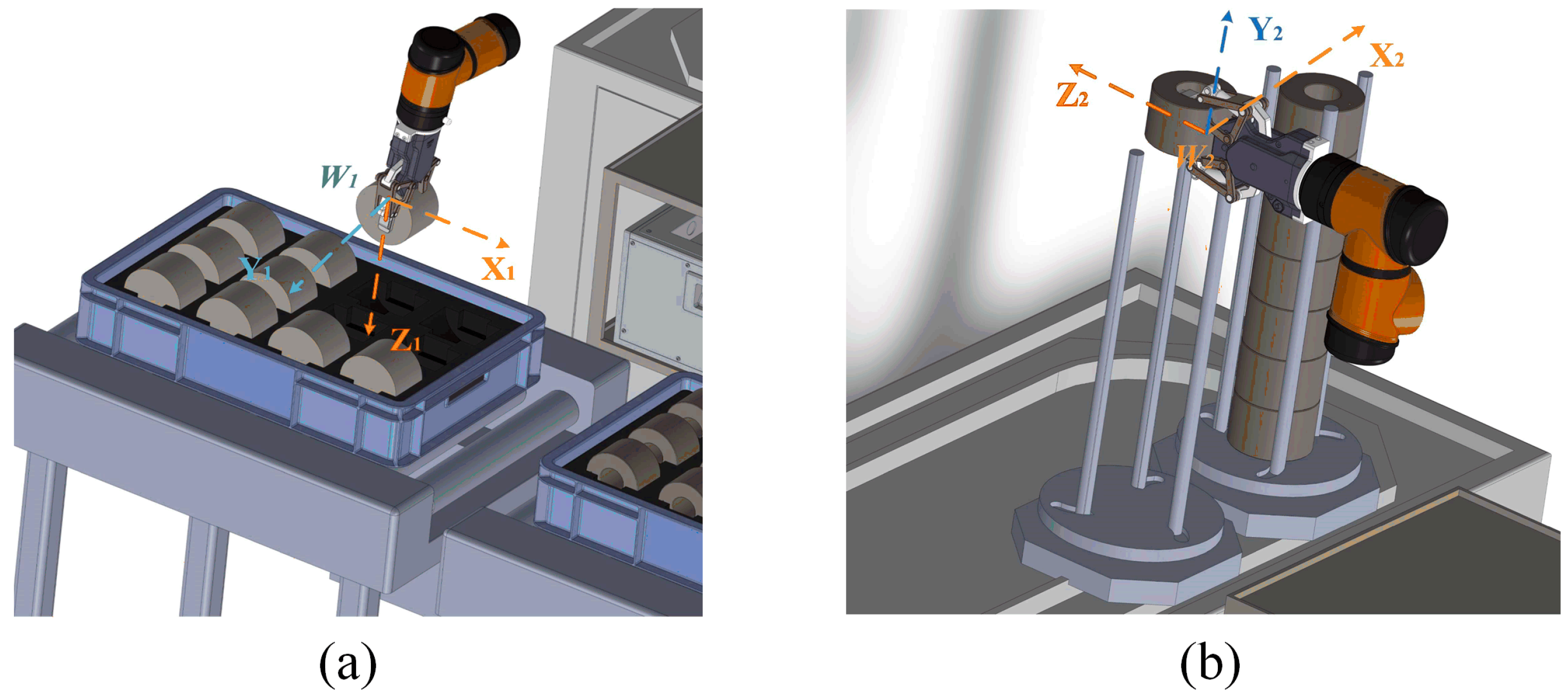This will comprehensively enhance the mechanization and automation levels of the coating industry [4]. Currently, among leading coating equipment manufacturers, the processing of aluminum plugs remains in a semi-automated production mode [5]. Although automated machining and clamping of aluminum plugs have been achieved with CNC turning centers and automated gantries, loading and unloading tasks still rely on manual operations, significantly restricting the production line’s processing efficiency [6]. To enhance industrial production and manufacturing efficiency, the robotic arm’s trajectory planning for loading and unloading aluminum plugs is essential. An appropriate trajectory interpolation algorithm can improve the operational stability of the robotic arm [7], while a time-optimal trajectory planning algorithm with dynamic adjustment strategies can further boost processing efficiency, reducing dependence on manual labor [8]. Therefore, trajectory planning and time optimization are crucial for enhancing operational safety, shortening the robotic arm’s loading and unloading time, and achieving a higher level of intelligent production. This study aims to address the scientific challenge of robotic arm trajectory planning during the automatic loading and unloading of aluminum block components in coating machinery. The scientific objective is to develop a time-optimal trajectory planning method based on a dynamically adaptive PSO algorithm to enhance operational efficiency and stability.

Currently, many scholars, both domestically and internationally, have conducted in-depth research on time-optimal, energy-optimal, and overall optimal trajectory planning for robotic arms, particularly for the time-optimal trajectory planning of six-degree-of-freedom robotic arms [9]. Based on the different methods used to describe motion states, there are two typical types of trajectory planning: joint-space trajectory planning and Cartesian-space trajectory planning [10]. Joint-space trajectory planning offers several advantages, such as simplicity in algorithms and high motion efficiency, and it typically avoids issues related to kinematic singularities [11]. Therefore, for trajectories without specific path constraints, planning in joint space should be given priority. Common joint space trajectory planning methods include polynomial interpolation, trapezoidal velocity interpolation, spline space interpolation [12], etc. Kielas-Jensen et al. [13] proposed a Bernstein polynomial-based method to convert infinite-dimensional optimization problems into non-linear programming problems for optimal trajectory generation, ensuring smooth and efficient motion planning. Boryga et al. [14] used asymmetric polynomial profiles for smooth trajectory planning, demonstrating their effectiveness in achieving smooth and efficient motion in robotic systems. Le Ying et al. [15] conducted trajectory planning for the REBOT-V-6R robot using quintic and septic non-uniform B-splines. The study demonstrated that trajectory planning with quintic and septic non-uniform B-spline curves results in smoother motion and higher planning accuracy. However, as the polynomial degree increases, the trajectory becomes more precise and smooth, but it may lead to the Runge phenomenon [16]. Therefore, to simplify computations while ensuring trajectory smoothness, the use of piecewise polynomial interpolation is a feasible approach.

Time-optimal trajectories refer to the motion paths of a six-degree-of-freedom robotic arm that completes a specific path in the shortest time within joint space. To achieve this, various trajectory optimization algorithms can be applied, such as Genetic Algorithm (GA) [17], Whale Optimization Algorithm (WOA) [18], Sparrow Search Algorithm (SSA) [19], Particle Swarm Optimization (PSO) [20], Ant Colony Optimization (ACO) [21], and others. Particle swarm optimization (PSO) has been widely applied to various engineering problems due to its advantages, such as few parameters, simple implementation, and strong applicability. However, the basic PSO algorithm suffers from issues such as slow convergence speed, the tendency to get trapped in local optima, and insufficient accuracy. To address these issues, many researchers have proposed improvements. Akopov [22] proposed a clustering-based hybrid particle swarm optimization algorithm for solving a multisectoral agent-based model, significantly improving optimization performance. Chen et al. [23] introduced a particle swarm optimizer with crossover operation, demonstrating its effectiveness in enhancing optimization accuracy and computational efficiency. Du et al. [24] proposed a trajectory planning method based on a piecewise interpolation function and the local chaotic particle swarm optimization (LCPSO) algorithm for the time-optimal trajectory planning problem in robotic arm motion. Ni et al. [25] transformed the coordinated trajectory planning problem of space robots into an optimization problem to find the optimal trajectory of the base and manipulator using Particle Swarm Optimization (PSO). Zhao et al. [26] introduced an improved hybrid method combining Whale Optimization and PSO algorithms, significantly improving the convergence speed. While these studies have made significant progress in the field of robotic arm trajectory planning, many still face challenges, such as high-order polynomials, complex calculations, and optimization algorithms being prone to premature convergence.

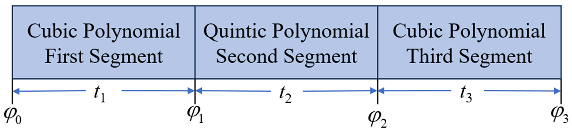
In summary, considering the actual production requirements and structural layout characteristics of the coating machine aluminum plug processing unit, how to ensure a smooth trajectory under the constraints of dynamic and geometric conditions while maintaining a small computational load, and how to integrate intelligent algorithms to achieve optimal results, thus improving the operational efficiency and stability of the robotic arm, is a critical technical challenge in the intelligent development of coating industry shaft-type parts production lines. Therefore, in order to improve the algorithm’s performance and reduce motion impact, this paper proposes a time-optimal trajectory planning method based on a dynamically adaptive PSO algorithm. The specific steps are as follows: First, the loading and unloading process of aluminum plug components in coating machinery is analyzed; then, a “3-5-3” hybrid polynomial interpolation method is used to fit the robotic arm’s loading and unloading trajectory; finally, the dynamically adaptive PSO algorithm is applied to optimize the trajectory, and the effectiveness of the proposed method is validated through experiments, achieving automatic loading and unloading of aluminum plug components in coating machinery and improving the processing efficiency of the production line.

2. Analysis of Loading and Unloading Process for Aluminum Plug Parts

2.1. Overview of Robotic Arm Loading and Unloading Conditions for Aluminum Plug Parts

Currently, the loading and unloading process for aluminum plug parts with a six-degree-of-freedom robotic arm in most coating and printing enterprises is illustrated in Figure 1, which includes two main scenarios:

(1) Part grasping and releasing condition: The robotic arm’s end effector moves from its initial position along a defined trajectory to points W₁ or W₂, where the gripper performs radial grasping or releasing of the aluminum plug or workpiece.

(2) Part transport condition: After the robotic arm completes the initial grasping of the part, it follows a pre-planned trajectory, moving between the storage box and the work platform to transport the part.

To distinguish between different states and facilitate subsequent discussions, this paper defines the robotic arm’s movement from the initial posture to the W₁ point for part grasping as condition 1 and the movement from the initial posture to the W₂ point for part grasping as condition 2.

2.2. Kinematic Analysis of the Robotic Arm’s Loading and Unloading Motion for Aluminum Plug Parts

To achieve the automated loading and unloading process of aluminum plug parts, the coordinate system origin of the robotic arm’s end effector needs to coincide with points W₁ and W₂ at specific poses. Therefore, a coordinate system has been established with W₁ and W₂ as reference points, as illustrated in Figure 2.

In this study, the AUBO i5 robotic arm is selected as the execution device for the automatic loading and unloading tasks. The coordinate system for each joint is established by setting the Z-axis as the joint’s rotation axis, with the Y-axis lying within the plane and the X-axis direction determined according to the right-hand rule. The kinematic structure diagram of the AUBO i5 robotic arm is shown in Figure 3.

The four basic geometric parameters of the AUBO i5 robotic arm based on the MD-H method are shown in

Table 1. MD-H Parameters of AUBO i5.

Link i	Link Length ai (m)	Link Angle αi (deg)	Link Offset di (m)	Joint Angle θi (deg)
1	0	0	0.1215	θ1
2	0	90	0.1405	90 + θ2
3	0.408	0	−0.1215	θ3
4	0.376	0	0.1025	−90 + θ4
5	0	−90	0.1025	θ5
6	0	90	0.094	θ6

.

Assuming that the six joints of the robotic arm rotate according to the parameters in Table 1, the origin of the end effector’s coordinate system can coincide with points W₁ and W₂. The parameters in

Table 2. Parameters of gripping points in joint space.

Coordinate Point	θ1		θ2		θ3		θ4		θ5		θ6
Unit	deg	rad	deg	rad	deg	rad	deg	rad	deg	rad	deg	rad
W1	−97.8	−1.7	−68.4	−1.19	−54	−0.94	32.4	0.56	90	1.57	−7.2	−0.12
W2	85.8	1.49	−32.4	−0.56	−36	−0.63	68.4	1.19	93.6	1.63	0.25	0.004

represent the joint space parameters used in the forward kinematics process of the robotic arm.

By performing forward kinematics analysis on the parameters in Table 2, the corresponding Cartesian space coordinates can be obtained. This represents the end-effector’s posture in the operational space when grasping the aluminum plug. The specific data are provided in

Table 3. Parameters of gripping points in operational space.

Coordinate Point	X (mm)	Y (mm)	Z (mm)	Roll (deg)	Pitch (deg)	Yaw (deg)
W1	−228.86	−775.43	−23.78	0.6	0	−180
W2	163.77	651.78	706.9	−180	0.6	−90
Initial endpoint	0	−215.1	1008.1	0	0	90

.

Under the parameters provided in the above two tables, the robotic arm’s motion to the grasping points during the automated loading and unloading process can be simulated using the built-in functions in the “Robotics Toolbox 10.4” plugin with MATLAB R2022a. The final result, as shown in Figure 4, demonstrates that the simulated posture matches the one shown in Figure 2.

3. Hybrid Polynomial Trajectory Planning

Trajectory planning for robotic arms in joint space focuses on describing the movement changes of each joint [27]. In joint space, the control input is torque, and the output is generalized joint coordinates [28]. This approach converts the joint angle variations of the robotic arm into time-based functions to describe its overall movement. The loading and unloading robotic arm in this study has six joints, meaning its joint space is six-dimensional, requiring six time-based functions to describe its overall movement. In polynomial trajectory planning, cubic polynomials have the advantages of low computational cost and simplicity, but they cannot constrain acceleration and may cause joint impacts. Quintic polynomials, on the other hand, offer more constraints, resulting in smoother interpolation but with higher computational cost. Therefore, this paper uses a “3-5-3” hybrid polynomial, which retains the low computational cost of the cubic polynomial while reducing joint impacts. Therefore, this paper uses a “3-5-3” hybrid polynomial for interpolation planning in joint space.

3.1. ”3-5-3” Hybrid Polynomial Trajectory Planning

A three-segment hybrid polynomial for interpolation fitting divides the joint angular displacement trajectory into three segments, as shown in Figure 5. In this scheme, the initial phase t₁ uses cubic polynomial planning, the middle phase t₂ uses quintic polynomial planning, and the final phase t₃ uses cubic polynomial planning. In addition, the starting point ${\phi }_0$ and the endpoint ${\phi }_3$, two intermediate interpolation points, ${\phi }_1$ and ${\phi }_2$, are required to complete the three-segment polynomial planning.

Let h(t) denote the joint angle displacement as a function of time t. Taking joint 1 as an example, the joint trajectory interpolation function for each segment is given as follows:

$$\left\{\begin{array}{l}{h}_1(t)=c_{10}+c_{11}t+c_{12}{t}^2+c_{13}{t}^3\\ h_2(t)=c_{20}+c_{21}t+c_{22}{t}^2+c_{23}{t}^3+c_{24}{t}^4+c_{25}{t}^5\\ h_3(t)=c_{30}+c_{31}t+c_{32}{t}^2+c_{33}{t}^3\end{array}\right.$$

(1)

In the equations, h_i(t) represents the angular displacement of the i-th polynomial segment at time t, c_ij denotes the j-th coefficient of the i-th function, and t refers to the interpolation time for each segment. By differentiating Equation (1) with respect to time, the expressions for the joint angular velocity (2) and angular acceleration (3) are derived:

$$\left\{\begin{array}{l}{\dot{h}}_1(t)=c_{11}+2c_{12}t+3c_{13}{t}^2\\ {\dot{h}}_2(t)=c_{21}+2c_{22}t+3c_{23}{t}^2+4c_{24}{t}^3+5c_{25}{t}^4\\ {\dot{h}}_3(t)=c_{31}+2c_{32}t+3c_{33}{t}^2\end{array}\right.$$

(2)

$$\left\{\begin{array}{l}{\ddot{h}}_1(t)=2c_{12}+6c_{13}t\\ {\ddot{h}}_2(t)=2c_{22}+6c_{23}t+12c_{24}{t}^2+20c_{25}{t}^3\\ {\ddot{h}}_3(t)=2c_{32}+6c_{33}t\end{array}\right.$$

(3)

To ensure a smooth transition of the displacement, velocity, and acceleration curves between segments in the hybrid polynomial interpolation method, appropriate constraints must be applied to the displacement, velocity, and acceleration. For instance, the final displacement, velocity, and acceleration of the h₁ segment should match the initial displacement, velocity, and acceleration of the h₂ segment. Similarly, the relationship between the h₂ and h₃ segments can be established. The constraints for the h₁ segment are given by the following Equation (4):

$$\left\{\begin{array}{l}{c}_{10}+c_{11}{t}_1+c_{12}{t}_1^2+c_{13}{t}_1^3=c_{20}\\ c_{11}+2c_{12}{t}_1+3c_{13}{t}_1^2=c_{21}\\ 2c_{12}+6c_{13}{t}_1=c_{22}\end{array}\right.$$

(4)

The constraints for the h₂ segment are given by the following Equation (5):

$$\left\{\begin{array}{l}{c}_{20}+c_{21}{t}_2+c_{22}{t}_2^2+c_{23}{t}_2^3+c_{24}{t}_2^4+c_{25}{t}_2^5=c_{30}\\ c_{21}+2c_{22}{t}_2+3c_{23}{t}_2^2+4c_{24}{t}_2^3+5c_{25}{t}_2^4=c_{31}\\ 2c_{22}+6c_{23}{t}_2+12c_{24}{t}_2^2+20c_{25}{t}_2^3=c_{32}\end{array}\right.$$

(5)

Since h₃ is the final polynomial segment, at the time t₃, its angular displacement should be ${\phi }_3$ as shown in Figure 5, and both the velocity and acceleration at t₃ should be zero. Therefore, the constraint conditions are given by the following Equation (6):

$$\left\{\begin{array}{l}{c}_{30}+c_{31}{t}_3+c_{32}{t}_3^2+c_{33}{t}_3^3={\phi }_3\\ c_{31}+2c_{32}{t}_3+3c_{33}{t}_3^2=0\\ 2c_{32}+6c_{33}{t}_1=0\end{array}\right.$$

(6)

At the starting time of the h₁ segment, the angular displacement is the initial value ${\phi }_0$, and both the velocity and acceleration should be zero. To ensure that the hybrid polynomial displacement trajectory passes through the interpolation points ${\phi }_1$ and ${\phi }_2$, the coefficients c₂₀ and c₃₀ must be set to ${\phi }_1$ and ${\phi }_2$, respectively. Therefore, the constraint conditions are given by the following Equation (7):

$$\left\{\begin{array}{l}{c}_{10}={\phi }_0\\ c_{11}=0\\ c_{12}=0\\ c_{20}={\phi }_1\\ c_{30}={\phi }_2\end{array}\right.$$

(7)

Equations (1)–(7) can be organized into a matrix expression as follows:

$$A\times a=\theta$$

(8)

where:

$$\begin{array}{c}A=\left[\begin{array}{ccc}B& C& 0\\ 0& D& E\\ 0& 0& F\\ G& 0& 0\\ 0& H& I\end{array}\right]\\ a=\left[\begin{array}{cccccccccccccc}{c}_{13}& c_{12}& c_{11}& c_{10}& c_{25}& c_{24}& c_{23}& c_{22}& c_{21}& c_{20}& c_{33}& c_{32}& c_{31}& c_{30}\end{array}\right]\\ \theta =\left[\begin{array}{cccccccccccccc}0& 0& 0& 0& 0& 0& {\phi }_3& 0& 0& {\phi }_0& 0& 0& {\phi }_2& {\phi }_1\end{array}\right]\end{array}$$

(9)

The matrix A is the time matrix, the matrix a contains the polynomial coefficients, and θ is the joint angle matrix, which includes the initial joint angle displacement, interpolation points, and final values. Where:

$$\begin{array}{cc}B=\left[\begin{array}{cccc}{t}_1^3& t_1^2& t_1& 1\\ 3t_1^2& 2t_1& 1& 0\\ 6t_1& 2& 0& 0\end{array}\right],\hfill & C=\left[\begin{array}{cccccc}0& 0& 0& 0& 0& -1\\ 0& 0& 0& 0& -1& 0\\ 0& 0& 0& -2& 0& 0\end{array}\right]\hfill \\ D=\left[\begin{array}{cccccc}{t}_2^5& t_2^4& t_2^3& t_2^2& t_2& 1\\ 5t_2^4& 4t_2^3& 3t_2^2& 2t_2& 1& 0\\ 20t_2^3& 12t_2^2& 6t_2& 2& 0& 0\end{array}\right],\hfill & E=\left[\begin{array}{cccc}0& 0& 0& -1\\ 0& 0& -1& 0\\ 0& -2& 0& 0\end{array}\right]\hfill \\ F=\left[\begin{array}{cccc}{t}_3^3& t_3^2& t_3& 1\\ 3t_3^2& 2t_3& 1& 0\\ 6t_1& 2& 0& 0\end{array}\right],\hfill & G=\left[\begin{array}{cccc}0& 0& 0& 1\\ 0& 0& 1& 0\\ 0& 1& 0& 0\end{array}\right]\hfill \\ H=\left[\begin{array}{cccccc}0& 0& 0& 0& 0& 0\\ 0& 0& 0& 0& 1& 0\end{array}\right],\hfill & I=\left[\begin{array}{cccc}0& 0& 0& 1\\ 0& 0& 0& 0\end{array}\right]\hfill \end{array}$$

(10)

3.2. “3-5-3” Hybrid Polynomial Trajectory Planning Simulation

This paper uses the “3-5-3” hybrid polynomial for interpolation of the robotic arm’s motion trajectory. In addition to the starting and ending points, two intermediate points (denoted as K₁, K₂ and L₁, L₂) are also required. Based on the data in Table 2, the six joint target angular displacements corresponding to points W₁ and W₂ are divided into three equal parts, resulting in data for the starting points, intermediate points, and target points, as shown in

Table 4. Interpolation points of mixed polynomial.

Coordinate Point	θ1		θ2		θ3		θ4		θ5		θ6
Unit	deg	rad	deg	rad	deg	rad	deg	rad	deg	rad	deg	rad
Initial point	0	0	0	0	0	0	0	0	0	0	0	0
K1	90	1.57	28.48	0.5	−40.9	0.71	−45	−0.79	−87.2	−1.52	−2.29	−0.04
K2	−13.1	−0.23	−22.5	−0.4	−7.3	−0.13	9.91	−0.79	2.69	0.05	4.59	0.08
W1	−97.8	−1.7	−68.4	−1.19	−54	−0.94	32.4	0.56	90	1.57	−7.2	−0.12
L1	62.9	1.1	10.7	0.19	−12	−0.21	62.9	1.1	31.1	0.54	−6.48	−0.11
L2	11.06	0.19	−15.6	−0.27	24.06	0.42	11.05	0.19	10.7	0.19	0.15	0.003
W2	85.8	1.49	−32.4	−0.56	−36	−0.63	68.4	1.19	93.6	1.63	0.25	0.004

. The initial point is the common starting posture for both working conditions. The path points for working condition 1 are composed of the initial point—K₁—K₂—W₁, and the path points for working condition 2 are the initial point—L₁—L₂—W₂.

Given that the planning time for each of the three segments is 2 s, and knowing the joint trajectory interpolation points and the planning time for each segment, the coefficient matrix α can be deduced using Formula (9) to obtain the coefficients for each joint. Since the hybrid polynomial consists of two cubic polynomials and one quintic polynomial, the trajectory planning curve for each joint will contain at most 14 coefficients. Additionally, since the initial conditions for joint motion include displacement, velocity, and acceleration constraints being zero, the constant term and the linear term coefficients for the first cubic polynomial are both zero. By substituting the data from Table 3 into Formulas (8) to (10), the coefficients for the hybrid polynomial can be determined. Based on these coefficients, the corresponding plots are shown in Figure 6, Figure 7 and Figure 8.

From the planned curve diagram, it can be seen that the “3-5-3” hybrid polynomial interpolation trajectory planning method combines the advantages of cubic and quintic polynomials. This approach avoids sudden changes in acceleration that can occur with cubic polynomials on complex paths, effectively addresses the high computational cost of higher-order polynomials, and enhances the motion efficiency and stability of the robotic arm’s end effector.

4. Time-Optimal Robotic Arm Trajectory Planning

4.1. Time-Optimal Trajectory Planning Based on Standard PSO Algorithm

Particle Swarm Optimization (PSO) is a typical heuristic algorithm that abstracts the numerical feasible solutions of a problem as individual particles, each with two attributes: position and velocity. The possibility of each particle reaching an optimal solution within the feasible domain is represented by its fitness. Each particle can remember all the positions it has visited and find the best position among them, which is the local optimum in the PSO algorithm. The best position reached by all particles in the entire swarm can be regarded as the global optimum, which is the global best solution in the PSO algorithm. Compared to other optimization algorithms, PSO has the advantage of particles sharing information with each other during the optimization process, allowing for faster convergence. In addition, PSO has a simple algorithm structure and easily adjustable parameters.

During the optimization process, each particle updates its position and velocity iteratively by tracking the local best solution and the global best solution. Suppose there are m particles searching for the optimal solution in a D-dimensional space, the position and velocity update formulas for the PSO algorithm are:

$$\left\{\begin{array}{l}{v}_{id}^{k+1}=w\cdot v_{id}^k+c_1\cdot r_1\cdot (p_{id}-x_{id}^k)+c_2\cdot r_2\cdot (g_d-x_{id}^k)\\ x_{id}^{k+1}=x_{id}^k+v_{id}^{k+1}\end{array}\right.$$

(11)

In the formula:

• w—Inertia weight, indicating the degree to which the particle’s velocity is influenced by its previous velocity during the update process;
• c₁—Local learning factor, indicating the statistical acceleration weight for the particle towards the local best position;
• c₂—Global learning factor, indicating the statistical acceleration weight for the particle towards the global best position;
• r₁, r₂—Pseudo-random numbers in the range [0, 1], used to increase the randomness in the optimization process;
• p_id—The local best position of particle i in the d-th dimension;
• g_d—The global best position of all particles in the current population in the d-th dimension;
• $x_{id}^k$—The d-dimensional position of particle i at the k-th iteration of the optimization;
• $v_{id}^k$—The d-dimensional velocity of particle i at the k-th iteration of the optimization.

From Equation (11), it can be observed that the particle’s velocity update includes three components: the memory term, the self-cognitive term, and the social-cognitive term. The memory term reflects the influence of the previous optimization result during the velocity update; the self-cognitive term indicates that the particle’s movement is influenced by its own experience; the social-cognitive term reflects the information sharing between particles, where the optimal position in the swarm is used to determine the next movement. The flowchart of the trajectory planning algorithm based on the standard PSO algorithm is shown in Figure 9.

The key to applying the Particle Swarm Optimization (PSO) algorithm in “3-5-3” hybrid polynomial trajectory planning lies in selecting the variables for particle optimization to obtain the optimal trajectory [29]. When optimizing the trajectory, if the polynomial coefficients in Equation (8) are chosen as the variables to be optimized, each joint’s trajectory polynomial would have a 14-dimensional optimization search space. By selecting time as the optimization variable, however, the total search space would have only three dimensions, significantly reducing both the computational load and code complexity. Based on Equation (8), given the time and joint angle displacements, the undetermined coefficient matrix a for each joint can be derived.

The objective of trajectory optimization, with joint movement time as the variable to be optimized, is to minimize the joint movement time under given constraints—this is time-optimal trajectory planning. This approach avoids complex mapping relationship calculations, limiting the search space to three dimensions. The fitness function and optimization constraints are then defined as follows:

$$\begin{array}{l}f(t)=\min (t_1+t_2+t_3)\hfill \\ s.t.\max \left\{\right|V_{j1}\left|\right\}\le V_{\max }\\ \hspace{1em} \max \left\{\right|V_{j2}\left|\right\}\le V_{\max }\\ \hspace{1em} \max \left\{\right|V_{j3}\left|\right\}\le V_{\max }\end{array}$$

(12)

In the formula:

• V_max—Maximum joint velocity;
• V_j1—Actual velocity of the first cubic polynomial segment for the j-th joint;
• V_j2—Actual velocity of the quintic polynomial segment for the j-th joint;
• V_j3—Actual velocity of the second cubic polynomial segment for the j-th joint.

When addressing multi-dimensional optimization problems, the standard PSO algorithm tends to get trapped in local optima, and its convergence speed can be relatively slow. The core issue lies in the fact that, typically, the inertia weight and learning factors in the standard PSO algorithm remain constant throughout iterations, leading to a fixed optimization search strategy. However, complex multi-dimensional optimization problems require a dynamic optimization strategy that can adaptively adjust parameters as the algorithm iterates. Therefore, this paper requires improvements to the standard PSO algorithm to adapt it for time-optimal trajectory planning of the “3-5-3” hybrid polynomial.

4.2. Time-Optimal Trajectory Planning Based on Dynamically Adaptive PSO Algorithm

The standard PSO algorithm relies on a fixed search strategy, making it difficult to adapt to dynamic environmental changes. In contrast, the dynamic adaptive PSO algorithm dynamically adjusts the particles’ search strategies and parameters, enabling it to more effectively search for the optimal trajectory in an ever-changing environment. By analyzing the search strategy of the PSO algorithm, we can summarize two key points that support improvements to the algorithm:

(1) Larger global search steps in early optimization: In the early stages of optimization, a larger global search step size is needed to increase the diversity of the population. Premature convergence in optimization algorithms typically occurs when the similarity among individuals in the population is high, leading to a rapid decline in diversity. If a “super individual” with a fitness value far exceeding the population average emerges, it can dominate the “reproduction rights” within the population.

(2) Enhanced local search ability in late optimization: In the later stages, when the population already has high diversity, the focus should shift to optimization precision and convergence speed. Stronger local search capabilities are therefore needed as the algorithm progresses. Adjusting to the changing iteration count, and increasing the local search step size in later optimization stages is crucial.

To address the above points, improvements are made to the inertia weight w, local learning factor c₁, and global learning factor c₂ in Equation (11). The inertia weight w, which represents the influence of the particle’s original velocity on its updated speed, affects the particle’s optimization ability. A non-linear dynamic function can be used to replace the constant inertia weight in the basic PSO algorithm, as shown in Equation (13):

$$w=w_{\min }+{\displaystyle \frac{(w_{\max }-w_{\min })\cdot n}{N}}$$

(13)

In the formula:

• w_min—minimum inertia weight;
• w_max—maximum inertia weight;
• n—current iteration count;
• N—maximum iteration count.

Similarly, a non-linear dynamic function is used as the fixed learning factor in the PSO algorithm, as shown in Equation (14):

$$\left\{\begin{array}{l}{c}_1=c_{\max }-(c_{\max }-c_{\min })\cdot {\sin }^2({\displaystyle \frac{\pi }{2}}\cdot (1-{\displaystyle \frac{1}{N}}))\\ c_2=c_{\min }+(c_{\max }-c_{\min })\cdot \sin ({\displaystyle \frac{\pi }{2}}\cdot {\displaystyle \frac{n}{N}})\end{array}\right.$$

(14)

In the formula:

• c_min—minimum learning factor;
• c_max—maximum learning factor;

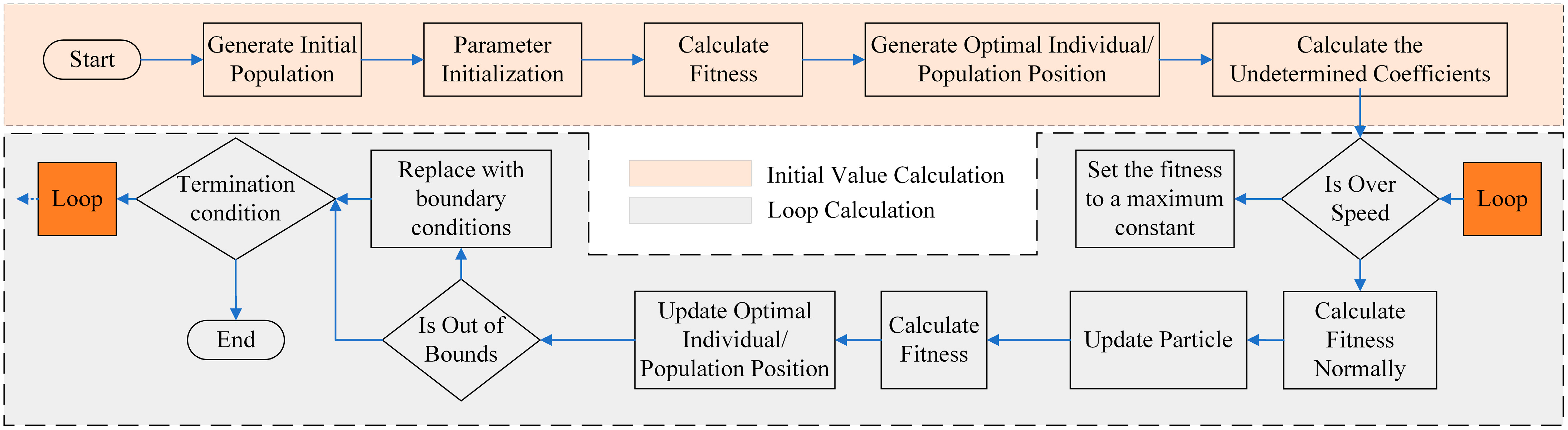
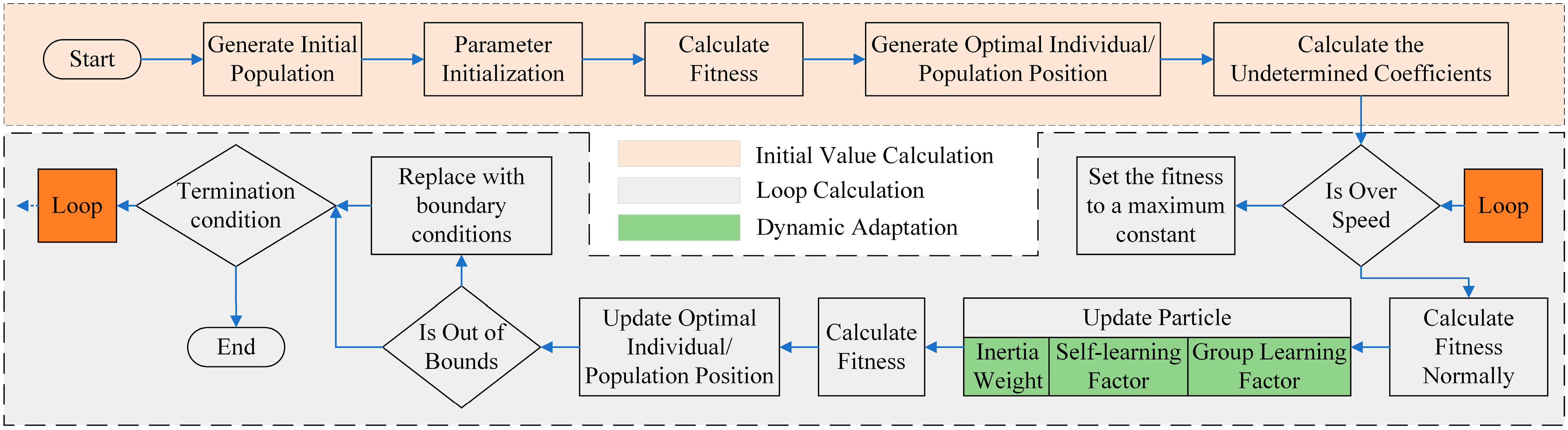
The process of the PSO algorithm with a dynamic adjustment strategy is shown in Figure 10.

The main difference between the improved PSO algorithm and the basic PSO algorithm is that the improved version has a dynamically adaptive particle update phase. This dynamic adaptability allows particles to adjust their search strategy based on the iteration count, improving the efficiency of the planning and better handling uncertainty, thereby meeting the real-time and accuracy requirements in practical applications.

4.3. Simulation Results and Analysis

In this paper, the maximum number of particles in the population is initialized to 20, with a maximum number of iterations set to 50. The initial individual learning factor c₁ and global learning factor c₂ are both set to 2. The minimum learning factor c_min is 1.5, and the maximum learning factor c_max is 2.5. The maximum inertia weight w_max is 0.9, and the minimum inertia weight w_min is 0.1. The algorithm’s search space has three dimensions. The solution space for each particle is within the range of [0, 2], and the velocity boundary for the particles is set to [−4, 4]. The maximum joint angular velocity is 5 rad/s. The initialization of the first-generation particle positions and velocities is given by the Formula (15):

$$\left\{\begin{array}{l}{x}_i=x_{\max }+rand(Pop,1)\cdot (x_{\max }-x_{\min })\\ v_i=rand(Pop,Dim)\end{array}\right.$$

(15)

In the formula:

• x_max—Upper limit of the particle solution space;
• x_min—Lower limit of the particle solution space;
• Pop—Maximum number of individuals in the population;
• Dim—Size of the optimization dimensions.

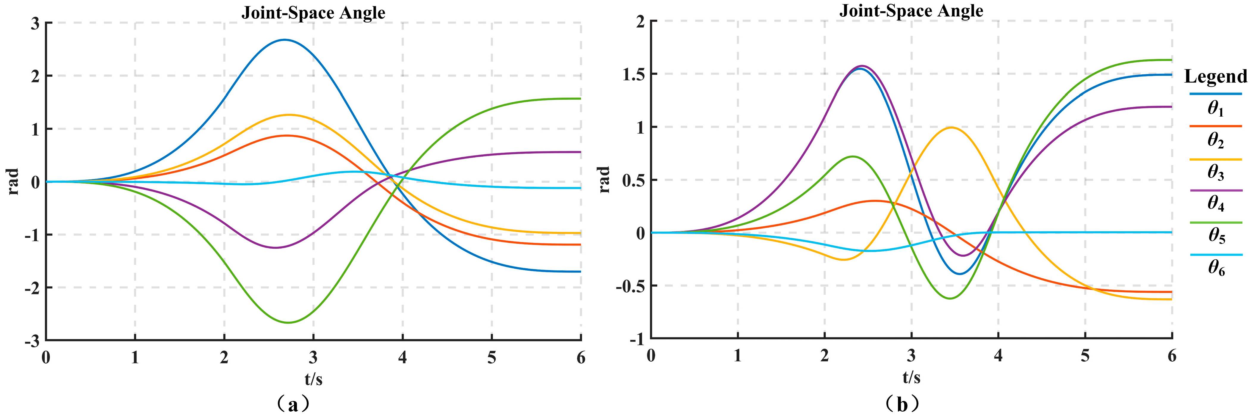
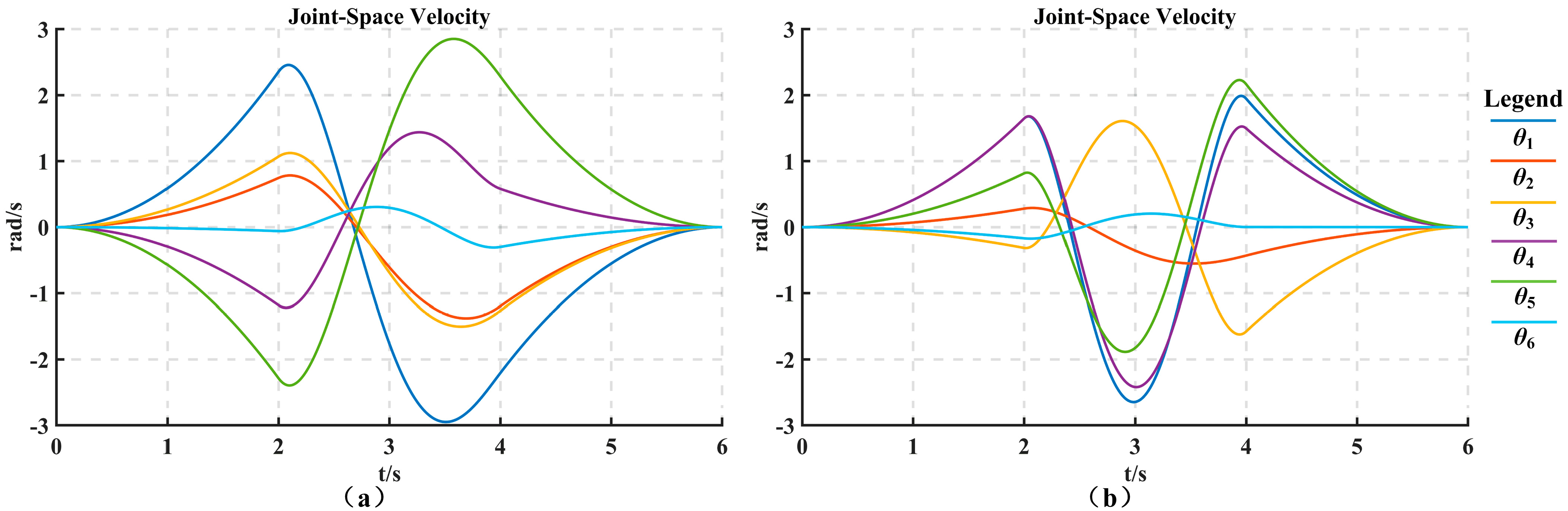
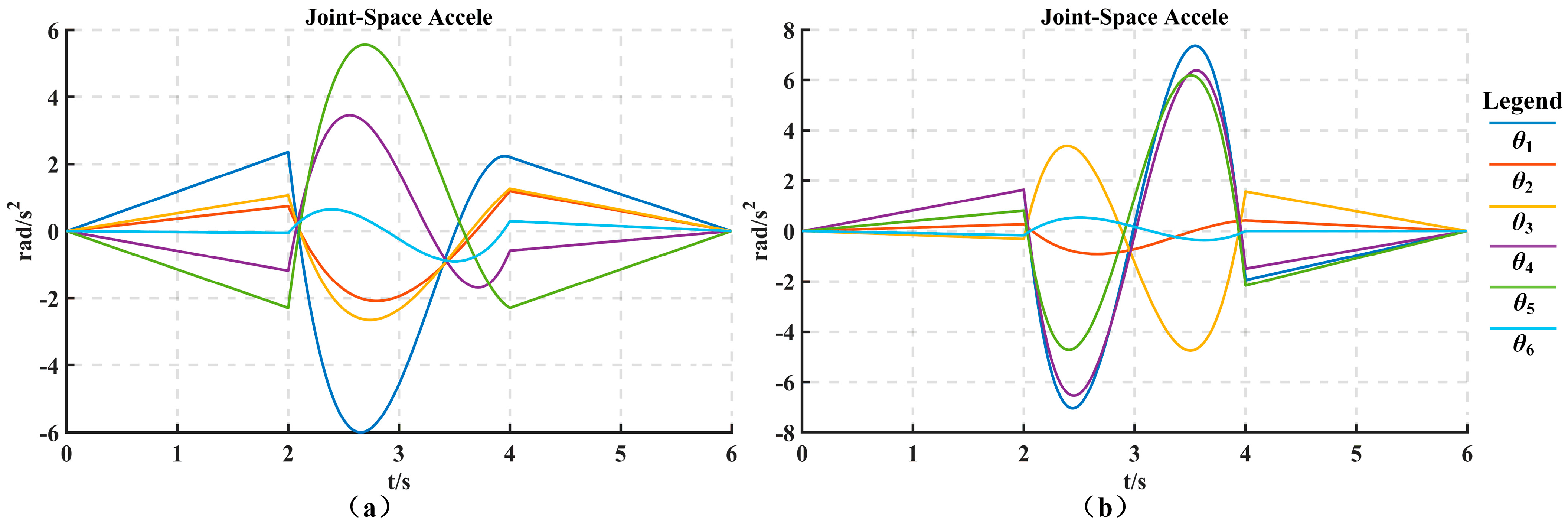
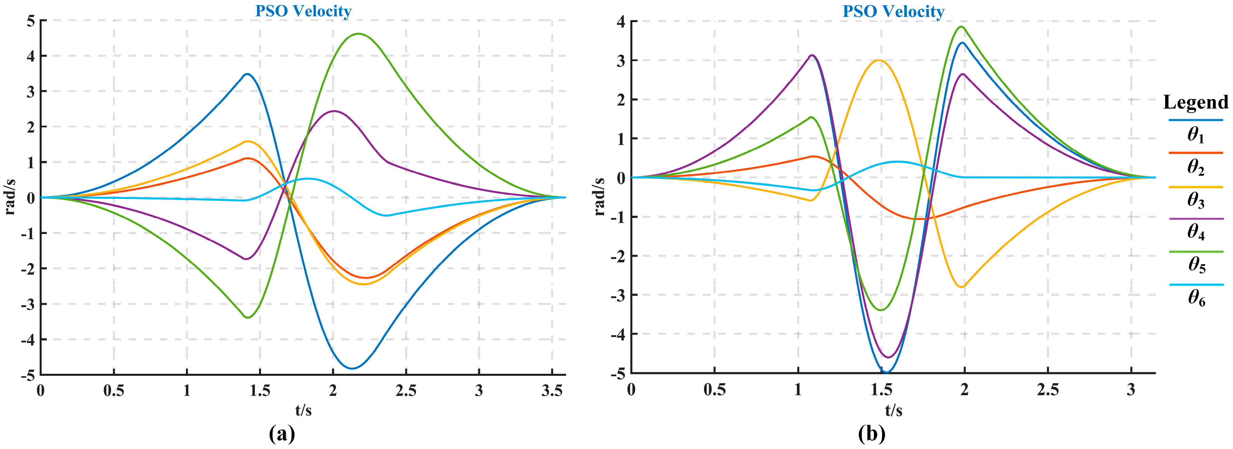
Based on the interpolation point data in Table 3, the optimal time trajectory planning was performed using the dynamic adaptive PSO algorithm proposed in this paper. The resulting joint angular displacement changes, joint angular velocity changes, and joint angular acceleration changes are shown in Figure 11, Figure 12, and Figure 13, respectively.

By comparing Figure 6 and Figure 11, it can be observed that the time-optimal trajectory planning proposed in this paper significantly reduces the time taken for all three stages of the “3-5-3” polynomial trajectory planning. The trajectory planning time of work condition 1 is reduced from 6 s to 3.59 s, resulting in an overall work efficiency improvement of 40.2%. Similarly, the trajectory planning time of work condition 2 is reduced from 6 s to 3.14 s, improving the overall work efficiency by 47.7%. The specific values are shown in

Table 5. Comparison table before and after optimization.

Enhanced Algorithm	First Stage	Second Stage	Third Stage	Total Time
Condition 1	1.41 s	0.95 s	1.23 s	3.59 s
Efficiency improvement	29.5%	52.5%	38.5%	40.2%
Condition 2	1.09 s	0.94 s	1.11 s	3.14 s
Efficiency improvement	45.5%	53%	44.5%	47.7%

.

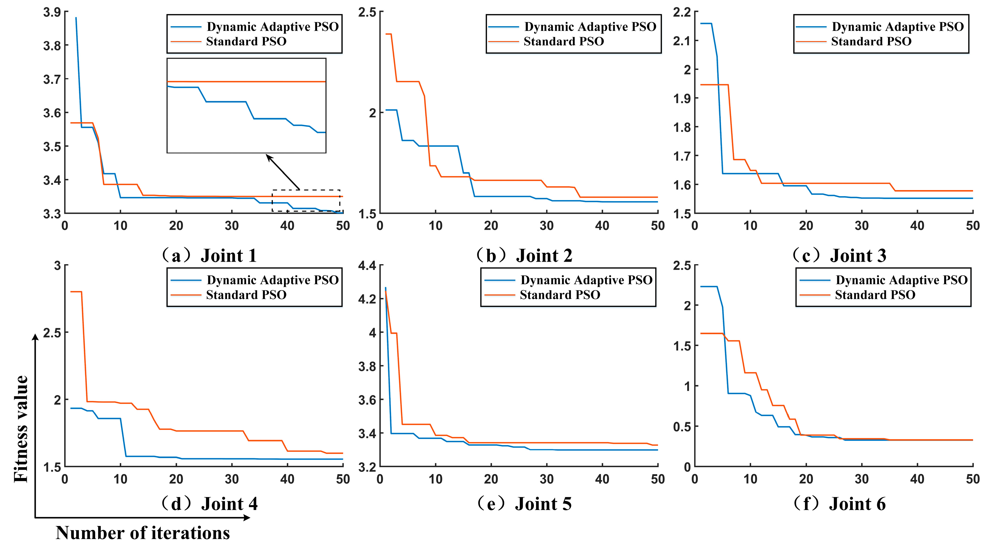
Fitness value is a metric used in genetic, evolutionary, or optimization algorithms to assess the quality of each candidate solution (individual). Figure 14 illustrates a comparison of fitness changes under condition 1 for the basic PSO algorithm and the improved dynamically adaptive PSO algorithm.

The adaptive PSO algorithm significantly improves fitness values and convergence time by dynamically adjusting the learning factors and inertia weight, balancing global and local search capabilities. Its optimization performance far exceeds that of the standard PSO. Analysis indicates that the proposed improved PSO algorithm is most effective in enhancing performance in the following two aspects:

(1) Significant Improvement in Fitness Values. The adaptive PSO algorithm achieves lower fitness values throughout the optimization process of all joints. For example, in subplot (a) of Figure 14, the fitness value of the standard PSO converges around 3.4, while the adaptive PSO further optimizes it to approximately 3.3. In subplot (c) of Figure 14, the fitness value of the standard PSO remains around 1.6, while the adaptive PSO reaches about 1.5. Subplots (b), (d), (e), and (f) in Figure 14 also show a significant downward trend, with the final fitness being better than that of the standard PSO. Therefore, the lower the fitness value, the better the performance of the objective function.

(2) Significant Acceleration of Convergence Time. The adaptive PSO demonstrates faster convergence in most joints. For example, in subplot (a) of Figure 14, the adaptive PSO converges after about 15 iterations, while the standard PSO takes approximately 40 iterations to converge. In subplot (d) of Figure 14, the adaptive PSO reaches stability within 10–20 iterations, while the standard PSO requires nearly 40 iterations. Subplots (b), (c), (d), (e), and (f) in Figure 14 also show a faster convergence trend, with the final convergence time being better than that of the standard PSO. Therefore, a faster convergence speed means that the algorithm can find high-quality solutions in a shorter time, improving computational efficiency and real-time performance, which is particularly important for robotic arm trajectory planning.

Based on the analysis of the results, it can be concluded that the time-optimal algorithm based on the dynamically adaptive PSO proposed in this paper significantly reduces the operating time of the robotic arm while satisfying maximum velocity constraints. Additionally, the time-optimal trajectory planning using the “3-5-3” hybrid polynomial allows for more flexible adjustments to changes in velocity and acceleration, making it suitable for trajectory planning in the loading and unloading tasks of the aluminum block by the robotic arm.

5. Summary

Aiming at the issue of low trajectory planning efficiency and high motion impact in the robotic arm’s loading and unloading tasks of aluminum blocks in coating machinery, this study proposes a time-optimal trajectory planning method based on a dynamically adaptive PSO algorithm. The main conclusions are as follows:

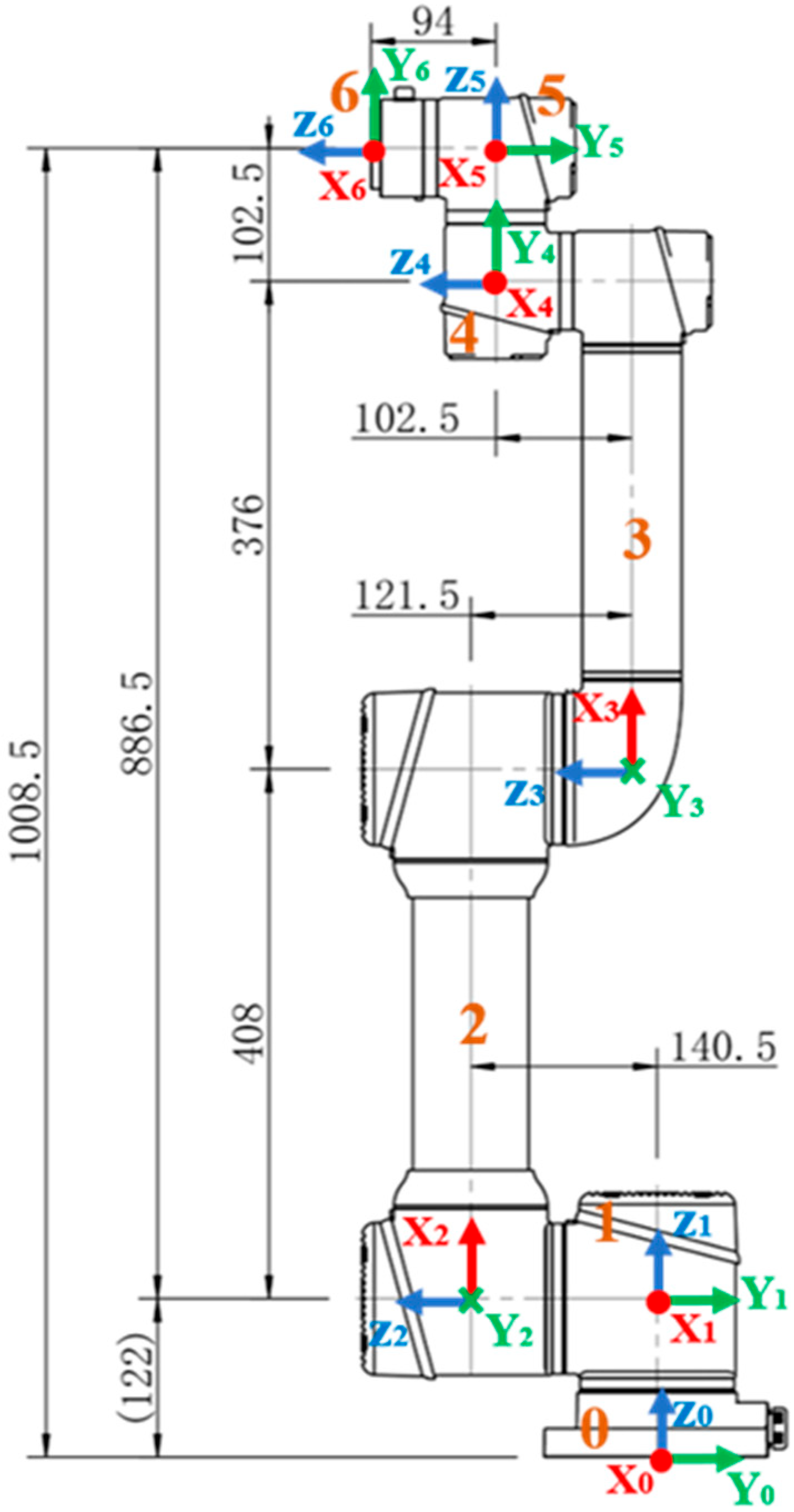
(1) Kinematic analysis of the robotic arm is conducted in joint space, and a “3-5-3” hybrid polynomial interpolation method is used to fit the motion trajectory. The results show that the “3-5-3” interpolation method effectively balances trajectory smoothness and kinematic performance, providing a stable foundation for robotic arm operation.

(2) By optimizing the robotic arm’s operation time as the objective function, the dynamically adaptive PSO algorithm is employed to minimize loading and unloading times, achieving time-optimal trajectory planning. This method significantly reduces the robotic arm’s operational time, thus improving efficiency. By optimizing the robotic arm’s operating time as the objective function, an improved dynamically adaptive PSO algorithm is employed to minimize the loading and unloading time, yielding the shortest trajectory for handling aluminum blocks, which is validated through simulation.

(3) Experimental results demonstrate that the “3-5-3” hybrid polynomial interpolation effectively balances path smoothness and kinematic performance. Furthermore, the time-optimal trajectory planning method based on the dynamically adaptive PSO reduces trajectory planning time from 6 s to 3.59 s and 3.14 s for condition 1 and condition 2, respectively, achieving efficiency improvements of 40.2% and 47.7%. These findings confirm the feasibility and effectiveness of the proposed method in enhancing the efficiency of automated aluminum block loading and unloading.

References

1. Lin, C.H. Implementation of China’s ’Replacing Humans with Machines’ Strategy to Promote Industrial Transformation Research. Dev. China. 2015, 15, 71–73. [Google Scholar]
2. Pendar, M.R.; Rodrigues, F.; Páscoa, J.C.; Lima, R. Review of Coating and Curing Processes: Evaluation in Automotive Industry. Phys. Fluids. 2022, 34, 101301. [Google Scholar] [CrossRef]
3. Xing, X.X.; Zhang, Y. Research on the Current Development Status and Strategies of China’s Robotics Industry. Sci. Technol. China. 2020, 11, 54–58. [Google Scholar]
4. Zhang, M.; Liao, Y. PID Parameter Optimization of Coating Machine Servo Injection System Based on PSO-SA Algorithm. Mach. Des. Manuf. 2024, 1–6. [Google Scholar]
5. China Packaging Federation. Development Prospects of China’s Printing Industry During the 14th Five-Year Plan Period. China Packag. 2021, 41, 22. [Google Scholar]
6. Liu, Y.C.; Jiang, Z.H.; Hu, J. Trajectory Planning and Simulation Research of a Six-DOF Robotic Arm Based on the ROS Platform. Manuf. Autom. 2022, 44, 38–41, 50. [Google Scholar]
7. Dong, L.; Yang, D.; Lu, J.S. A Review of Industrial Robot Trajectory Planning Methods. Control Eng. 2022, 29, 2365–2374. [Google Scholar]
8. Wei, B.; Shu, S.H.; Zhang, Y.; Yang, R.; Xing, B. Kinematics Analysis and Trajectory Planning Simulation of Manipulator Based on AUBOI5. In Proceedings of the 4th Annual International Conference on Data Science and Business Analytics, Changsha, China, 5–6 September 2020; pp. 72–75. [Google Scholar]
9. Cao, J.Q.; Han, X.S. Research Methods for Trajectory Planning of Industrial Robots: A Review. Inf. Control. 2024, 53, 471–486+498. [Google Scholar]
10. Xiong, R.; Zhan, J.B.; Tang, Q.; Chu, J. Time-Optimal Control of Mobile Robots with Velocity and Acceleration Saturation Constraints. Control Decis. 2014, 29, 118–122. [Google Scholar]
11. Li, W.; Deng, C.H.; Ge, J.M.; Liu, W.; Li, C.Y. Research Progress on Robot Joint Space Trajectory Planning. Mech. Des. Manuf. Eng. 2022, 51, 15–23. [Google Scholar]
12. Jia, X.; Zhao, B.; Liu, J.; Zhang, S. A Trajectory Planning Method for Robotic Arms Based on Improved Dynamic Motion Primitives. Ind. Robot Int. J. Robot. Res. Appl. 2024, 51, 847–856. [Google Scholar] [CrossRef]
13. Boryga, M.; Kołodziej, P.; Gołacki, K. The Use of Asymmetric Polynomial Profiles for Planning a Smooth Trajectory. Appl. Sci. 2022, 12, 12284. [Google Scholar] [CrossRef]
14. Kielas-Jensen, C.; Cichella, V.; Berry, T.; Kaminer, I.; Walton, C.; Pascoal, A. Bernstein Polynomial-Based Method for Solving Optimal Trajectory Generation Problems. Sensors 2022, 22, 1869. [Google Scholar] [CrossRef]
15. Le, Y.; Yue, Y.B. Kinematics Simulation and Trajectory Planning of Six-DOF Robot. Modular Mach. Autom. Process. Technol. 2016, 4, 89–92. [Google Scholar]
16. Zhang, X.; Xiao, F.; Tong, X.; Yun, J.; Liu, Y.; Sun, Y.; Tao, B.; Kong, J.; Xu, M.; Chen, B. Time-Optimal Trajectory Planning Based on Improved Sparrow Search Algorithm. Front. Bioeng. Biotechnol. 2022, 10, 852408. [Google Scholar]
17. Katoch, S.; Chauhan, S.S.; Kumar, V. A Review on Genetic Algorithm: Past, Present, and Future. Multimedia Tools Appl. 2021, 80, 8091–8126. [Google Scholar] [CrossRef] [PubMed]
18. Mirjalili, S.; Lewis, A. The Whale Optimization Algorithm. Adv. Eng. Software 2016, 95, 51–67. [Google Scholar] [CrossRef]
19. Xue, J.; Shen, B. A Novel Swarm Intelligence Optimization Approach: Sparrow Search Algorithm. Syst. Sci. Control Eng. 2020, 8, 22–34. [Google Scholar] [CrossRef]
20. Mazhoud, I.; Hadj-Hamou, K.; Bigeon, J.; Joyeux, P. Particle Swarm Optimization for Solving Engineering Problems: A New Constraint-Handling Mechanism. Eng. Appl. Artif. Intell. 2013, 26, 1263–1273. [Google Scholar] [CrossRef]
21. Fang, S.P.; Ru, Y.; Liu, Y.Y.; Hu, C.M.; Chen, X.Y.; Liu, B. Route Planning of Helicopters Spraying Operations in Multiple Forest Areas. Forests 2021, 12, 1658. [Google Scholar] [CrossRef]
22. Akopov, A.S. A Clustering-Based Hybrid Particle Swarm Optimization Algorithm for Solving a Multisectoral Agent-Based Model. Stud. Inform. Control 2024, 33, 83–95. [Google Scholar] [CrossRef]
23. Chen, Y.; Li, L.; Xiao, J.; Yang, Y.; Liang, J.; Li, T. Particle Swarm Optimizer with Crossover Operation. Eng. Appl. Artif. Intell. 2018, 70, 159–169. [Google Scholar] [CrossRef]
24. Du, Y.; Chen, Y. Time Optimal Trajectory Planning Algorithm for Robotic Manipulator Based on Locally Chaotic Particle Swarm Optimization. Chinese J. Electron. 2022, 31, 906–914. [Google Scholar] [CrossRef]
25. Ni, S.; Chen, W.; Ju, H.; Chen, T. Coordinated Trajectory Planning of a Dual-arm Space Robot with Multiple Avoidance Constraints. Acta Astronautica 2022, 195, 379–391. [Google Scholar] [CrossRef]
26. Zhao, J.; Zhu, X.; Song, T. Serial Manipulator Time-Jerk Optimal Trajectory Planning Based on Hybrid IWOA-PSO Algorithm. IEEE Access 2022, 10, 6592–6604. [Google Scholar] [CrossRef]
27. Choi, Y.; Kim, D.; Hwang, S.; Kim, H.; Kim, N.; Han, C. Dual-Arm Robot Motion Planning for Collision Avoidance Using B-Spline Curve. Int. J. Precis. Eng. Manuf. 2017, 18, 835–843. [Google Scholar] [CrossRef]
28. Wang, Q.Z.; Yin, C.W. A New Derivation and Solution Method for the Inverse Kinematics Equation of the Puma Manipulator. Robot 1998, 20, 81–87. [Google Scholar]
29. Fu, R.; Ju, H.H. Time-Optimal Trajectory Planning Algorithm for Robotic Arms Based on Particle Swarm Optimization. Inf. Control 2011, 40, 802–808. [Google Scholar]
Figure 1. Schematic diagram of loading and unloading.
Coatings 15 00002 g001
Figure 2. Establishment of a coordinate system for two points. (a) The coordinate system of point W1; (b) The coordinate system of point W2.
Coatings 15 00002 g002
Figure 3. The kinematic structure diagram of the AUBO i5 robotic arm.
Coatings 15 00002 g003
Figure 4. Gripping pose of the robotic arm. (a) The end-effector posture corresponding to Point W1; (b) The end-effector posture corresponding to Point W2.
Coatings 15 00002 g004
Figure 5. “3-5-3” Hybrid polynomial trajectory planning illustration.
Coatings 15 00002 g005
Figure 6. “3-5-3” Mixed polynomial joint angle displacement curve. (a) Angular displacement for condition 1; (b) Angular displacement for condition 2.
Coatings 15 00002 g006
Figure 7. “3-5-3” Mixed polynomial joint velocity curve. (a) Angular velocity for condition 1; (b) Angular velocity for condition 2.
Coatings 15 00002 g007
Figure 8. “3-5-3” Mixed polynomial joint acceleration curve. (a) Angular acceleration for condition 1; (b) Angular acceleration for condition 2.
Coatings 15 00002 g008
Figure 9. Time-optimal trajectory planning based on standard PSO algorithm.
Coatings 15 00002 g009
Figure 10. Time-optimal trajectory planning based on dynamic adaptive PSO algorithm.
Coatings 15 00002 g010
Figure 11. Dynamic adaptive PSO joint angle displacement curve. (a) Angular displacement for condition 1; (b) Angular displacement for condition 2.
Coatings 15 00002 g011
Figure 12. Dynamic adaptive PSO angular velocity curve. (a) Angular velocity for condition 1; (b) Angular velocity for condition 2.
Coatings 15 00002 g012
Figure 13. Dynamic adaptive PSO angular acceleration curve. (a) Angular acceleration for condition 1; (b) Angular acceleration for condition 2.
Coatings 15 00002 g013
Figure 14. Comparison of fitness changes under working condition 1.
Coatings 15 00002 g014