Abstract
Maintaining the temperature of liquid steel in the ladle in the required range affects the quality of casted billets, reduces energy consumption, and guarantees smooth control of the melting sequence. Measuring its temperature is a challenging task in industrial settings, often hindered by safety concerns and the expensive nature of equipment. This paper presents models which enable the prediction of the cooling rate of liquid steel for variable production parameters, i.e., steel grade and weight of melt. The models were based on the FEM solution of the Fourier equation, and machine learning approaches such as decision trees, linear regression, and artificial neural networks are utilized. The parameters of the model were identified using data from the monitoring system and inverse analysis. The results of simulations were verified with measurements performed in the production line.
1. Introduction
The constant increase in demand for high-quality steels and energy savings are the main factors that drive the ongoing continuous optimization of the steelmaking process, while both the quality of steel as well as efficiency of this process strongly depend on the temperature of the liquid metal. Too low a temperature can lead to metal freezing, which results in clogging of tipping hole, or at a later stage of the process in freezing of the band during the continuous casting of steel, causing a long-term interruption in manufacturing. The overheating of liquid steel causes unfavorable structural changes in the steel, accelerates the wear of the refractory lining of the ladle furnace and tundish, and increases energy consumption. The model enabling the prediction of the cooling rate of liquid steel, as part of a larger cyber-physical system, can be used both to create a plan of the melting sequence and to control the production process in real time. Most of the solutions found in the literature concern three stages of the steelmaking process: steel melting in an arc furnace [1], refining [2], and continuous steel casting [3]. On the other hand, the analysis of heat loss in ladles is primarily considered in terms of their design. Such a model was presented in the paper [4], in which the optimal parameters of the ladle lining for minimal energy consumption were determined. The presented model describes the heat transfer in molten steel during the transport of the ladle (Figure 1) between the stations. Refining tundish allows for the determination of the temperature of liquid steel for variable production parameters, i.e., steel grade and weight of melt. Predicting the temperature at which the ladle arrives at the continuous casting station (CST) is critical to planning for overheating during pouring and maintaining the right time to leave the ladle metallurgical station (LMS) station.

Figure 1.
A flow diagram of the steel manufacturing process.
There are many successful applications of machine learning models in the metallurgical industry. In [5], authors created a model of a blister copper two-stage production process. Each stage (copper flash smelting process and converting of copper matte) was modeled using three techniques: artificial neural network, support vector machine (SVM), and random forest (RF). To assess the influence of measurement errors on the model’s accuracy, the training was conducted four times using data with varying levels of noise (representing 0%, 2%, 5%, and 10% fluctuations in parameter values). The fitting accuracy of random forest (RF) significantly lagged behind that of the artificial neural network (ANN) and support vector machine (SVM) models.
The fitting error of the support vector machine exceeds that of the artificial neural network, although the disparity between these two methods diminishes when the training data are subjected to random perturbations. This implies that SVM could serve as a viable alternative to ANN when dealing with noisy industrial data. Kusiak et al. in [5] delved into the concept of data-driven models and provides a comparative analysis of the efficacy of three techniques: response surface methodology, kriging method, and artificial neural networks. The authors compared the accuracy of the investigated modelling techniques using two test functions and the process of laminar cooling (LC) of dual phase (DP) steel strips after hot rolling. The training of each model was performed using three datasets which consisted of different numbers of points. The obtained results showed that the ANN-based model of the LC process had the lowest error and that it can be applied in further optimization computations. The authors constructed an artificial-neural-network-based model to simulate the oxidizing roasting process of zinc sulfide concentrates. This model successfully projected the sulfide sulfur concentration in the roasted ore, incorporating both the chemical composition of zinc concentrate and the selected parameters of the roasting procedure. The model’s precision was assessed through utilization of the root mean square error (RMSE), which amounted to approximately 5%.
The presented models operate on real production data, while those presented in the literature often refer to experimental melts in a controlled environment. In this context, as well as in the face of the fact that the models are now being implemented in a real industrial process, we face here the problems of adapting to real conditions, and not only to theoretical considerations about phenomena.
2. FEM Solution of Fourier Equation
The steelmaking process in the electric arc furnace (EAF) begins with the charging of scrap. After melting, the liquid steel is tapped into the ladle and transported to ladle furnace stations (LMS) where the operations of refining and reheating are performed. In the next step of the process, the ladle is moved to the continuous steel casting station (CC) (Figure 2).

Figure 2.
Scheme of the ladle furnace: 1—armor, 2—insulation layer, 3—lining, 4—molten steel, 5—slag.
The presented model allows for the prediction of the temperature of liquid steel during this transport. The FEM solution of the Fourier Equation (1) was carried out in the 2D system.
where: r is the material density, cp is the specific heat of the material, and k is coefficient of heat conduction of material. The boundary conditions adopted in the model are as follows.
- The temperature of the inner surface of the ladle is equal to the temperature of the molten steel.
- The heat transfer inside liquid steel, insulation layer, and lining is carried out by conduction
- The heat transfer from the outer surface of the ladle and the slag layer occurs by convection (qc) and radiation (qr):
Input data, including the temperature of molten steel measured after the refining process, the temperature of ladle armor, and transport time, were received from the monitoring system. The weight of the molten steel was 140 tons. The values of the thermophysical parameters introduced into the model are summarized in Table 1. The data for the lining came from the material cards. The thermal conductivity coefficient of the slag was determined on the basis of experimental studies. The specific heat and emissivity data for each of the materials were from the literature data. Discretization of the calculation domain was performed for 3-node triangular elements; the time period was equal to 0.1.

Table 1.
Thermophysical parameters.
Numerical simulations were carried out for steel grades for which numerous industry data sets were available, which facilitated verification of the correctness of the results, i.e., unalloyed structural steels: S235JR, S355J2, STRETCH500, rein-forcing steels: B500SP, B500B; quenching and tempering steel: C45E; alloy special steel: 30MnB4; and steel for carburizing: 16MnCrS5. The duration of data collection was 14 months. The results of simulations are shown in Figure 3. The cooling rate was calculated using the relationship cr = (TLF − Tcc)/ttransport, where TLF is the temperature at the LF station, Tcc is the temperature at the CC station), and ttransport is the time of transport. The verification of the obtained results was carried out on the basis of measurement data from the monitoring system. The place of temperature verification corresponds to the place where the measurement in industrial conditions was carried out (average value of three measurements). The cooling rate varied within the range of 1.18 °C/min for STRETCH500 steel and 1.39 °C/min for 16MnCr5 steel. The mean relative error of the calculations was in the range of 0.12–0.18 and was the lowest for steel 30MnB4 and the highest for steel S235JR.
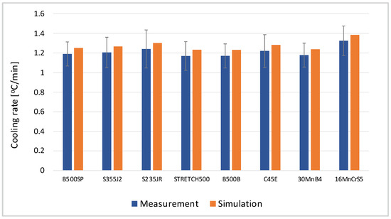
Figure 3.
Cooling rate of liquid steel by comparison of calculated (orange column) and filtered measurement data (blue column).
The temperature distribution in the molten steel is presented in Figure 4. In all the analyzed cases, the temperature drop was observed only under the slag layer and in the contact zone with the ladle lining.
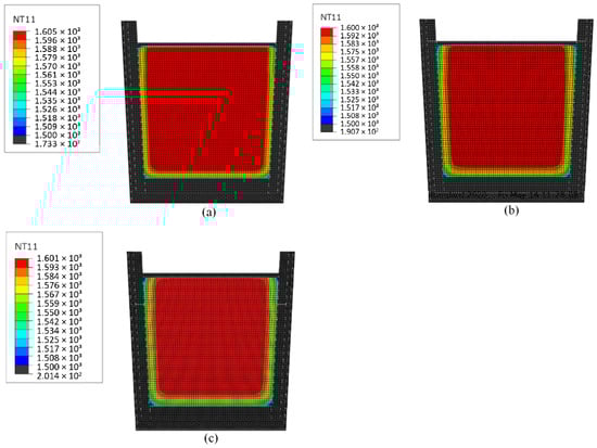
Figure 4.
Temperature distribution in the molten steel—16MnCr5 steel: (a) melt I—1587 °C, 19 min; (b) melt II—1570 °C, 18 min; (c) melt III—1607 °C, 10 min.
The model allows for the determination of the liquid steel cooling rate in the main ladle. The measurements of temperature in the ladle confirm the correctness of the model. Due to the long computation time of ~35 min, it was necessary to create a metamodel that would enable the use of the prediction model in industrial conditions.
3. Statistical Data Analysis and Decision Trees
The purpose of the statistical analysis and the use of decision trees was to determine the relationships visible in the collected data. The objective was to discover the stochastic relationship between the measured parameters of the cooling process and the change in temperature of the metal in the ladle over time. The variables used in the analysis were initial temperature, cooling time, molten metal mass, ladle weight, temperature difference, and cooling rate.
3.1. Statistical Data Analysis
The data were collected during production over a period of 14 months. Each record represents one heat which is approximately 145 tons of steel. The data were noisy and highly variable, ranging from anomalies to missing data. In some cases, it was suspected that there was no proper initial temperature measurement. The characteristics of the collected data are daily production, often disturbed by events on the line, as well as factors independent of the production processes. The scatter of the data is well illustrated by the scatter plots shown in Figure 5. The analyses were carried out using the STATISTICA package.
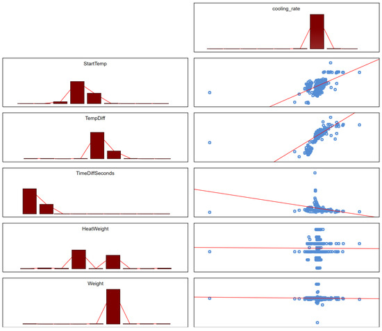
Figure 5.
Scatterplots between the parameters of the cooling process and the cooling rate. The red lines represent linear regressions for one pair of variables (simple regression) and are therefore the best visualization of the correlation coefficient. The histogram columns represent the number of observations in individual ranges of the variable scale, while the blue dots represent data points in the feature space.
In order to increase the reliability of future models and to separate the measurements burdened with anomalies, the data were cleaned, eliminating outliers (according to the three-sigma rule). In the normality plots shown in Figure 6a,b and Figure 7a,b, it can be seen that after cleaning the noisy data approached the normal distributions, as would be expected. After cleaning, the dataset included 7362 heats.
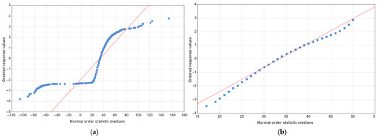
Figure 6.
Temperature difference normality plots in (a) the raw data set and (b) in the cleaned data set. The red lines represent linear regressions, while the blue dots represent data points.
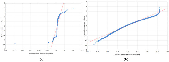
Figure 7.
The cooling rate normality charts (a) in the raw data set and (b) in the cleaned data set. The red lines represent linear regressions, while the blue dots represent data points.
In the traditional approach to statistical methods, the F-test is used to test the dependence of variables in multivariate analyses. This test shows how strongly the variables are related to the dependent variable. The test results for the cooling rate can be read from Figure 8.
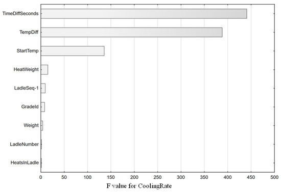
Figure 8.
F-test results for cooling rate.
The F-test indicated that the most important variables affecting the cooling rate were the cooling time, the temperature difference, the initial cooling temperature and, to a negligible extent, the mass of the metal bath. The influence of the weight is negligible due to the small variability of this parameter. We can follow the course of these relationships in the scatterplots which confirm these results. Figure 9 shows the scatterplots for the data after cleaning.
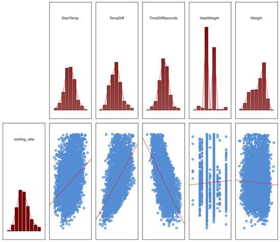
Figure 9.
Scatterplots for cleanup data for selected factors.
It is worth noting that the HeatWeight index was not included due to its discrete nature related to the boundary conditions of the process, instead, in further analyses, the weight of the metal bath was included in Weight. The created models also did not take into account one of the strongest predictors—temperature change, due to the fact that this parameter is known only after cooling and does not allow for prediction, and since it is basically the basis for determining the cooling rate in calculations, hence it cannot be treated as a predictor.
Among the discrete factors, the steel grade should be established as a factor that undoubtedly has a technological influence on the cooling rate. However, in the case of this factor, it is difficult to speak of a statistically reliable impact, due to the fact that the size of the collection was clearly unevenly distributed between grades. The production data mostly included a few of the most common materials, and some grades were represented only by single heats. The differences in the cooling rate index for different grades are shown in Figure 10.
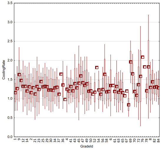
Figure 10.
Box-plot cooling rate charts for individual steel grades.
3.2. Regression Trees
To explore the correlation between continuous and discrete parameters, and to make an attempt at predicting the cooling rate, the modeling process began with the utilization of regression trees. Regression trees, which belong to the decision tree induction family, are employed when the dependent (target) variable is continuous. These trees are a favored algorithm for prediction due to their interpretability. They offer a human-friendly way of presenting relationships through graphical representations, specifically in the form of a graph denoted as G = (V, E). In this structure, V signifies a finite non-empty set of nodes (vertices), while E denotes a set of edges (leaves). In the graph, the nodes within the structure represent sets and subsets (data partitions), while the edges symbolize the conditions (partition tests) applied to the individual partitions [6]. To predict the value of the dependent variable for a given instance, users navigate the decision tree. Commencing from the root, they follow edges based on attribute test outcomes. Upon reaching a leaf, the information stored in that leaf dictates the prediction’s outcome. For instance, in a regression problem, this outcome encompasses the mean of the node as well as the standard deviation or variance within that node (partition) [7].
The prevalent technique for crafting decision trees involves an induction algorithm known as top-down induction, which employs a greedy, recursive, top-down strategy to partition the tree [8]. To generate accurate decision trees, proficient algorithms have been developed. Typically, these algorithms utilize greedy methods to construct decision trees in a top-down manner. This involves making a sequence of locally optimal decisions concerning attribute selection for the training set partitioning and internal attribute splitting. Hunt’s Concept Learning System Framework, one of the earliest decision tree induction algorithms, underpins several contemporary methods such as ID3, C4.5, and CART. These induction algorithms for decision trees are extensively documented in the literature, as seen in references [9,10]. The form of the tree derived from the training dataset through v-cross validation can be depicted through the graph illustrated in Figure 11.

Figure 11.
Tree form obtained from the training dataset using CART algorithm and v-cross validation. The numbers represent the ID of each node. The individual nodes are marked in blue, while the final leaves are marked in red.
The quality of the model is assessed, as in other machine learning models, by fitting the model indications to the actual values. The visual evaluation of the model can be seen in the scatter plot of predicted and actual values (Figure 12). We observe a characteristic arrangement of the predicted values. The predictions are discrete and arranged in lines. This is the effect of the model. The prediction is the same for the whole group of cases from one leaf. If the conditions (tests on attributes) are met, the model returns in the prediction the mean value of the dependent variable appropriate for this partition, hence the abrupt change in prediction. The nature of regression trees is thus essentially discrete, not continuous. The result of this approach is lower precision than in other models, such as linear regression or neural networks, but the main advantage of these trees is their ability to explain dependencies. Hence, it is prudent to delve into the intricate details of the outcomes.
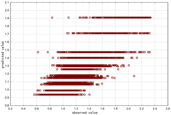
Figure 12.
Scatterplot of predicted and actual values for the CART model.
The quantitative assessment of regression tree models can be described by error indicators such as MAE (mean absolute error) or R2 (coefficient of determination). In the presented model, these indicators were, respectively: MAE = 0.13, R2 = 0.62 (Table 2). Although the fitting measured by the coefficient of determination is imperfect (due to the nature of the trees, which was mentioned previously), the MAE error is small. This means that the predictions made with the use of this model do not differ significantly from the real values.
Table 2.
Assessment of the adjustment of the CART model predictions to the real values.
The nodes at the end of each branch are called leaves. Each leaf represents a data partition that satisfies the rationale of tests on attributes (predictors). Since the CART tree is a binary tree, a given attribute may be used more than once in the tests. The readiness to take part in the attribute test is each time assessed using the criterion function verifying the significance of the attribute, that is its discriminatory power. If the variance in the child nodes decreases after partitioning, the attribute is ranked higher. The more it reduces the post-partition variance, the more important it is. The assessment of the importance of predictors in the developed model is presented in Figure 13. The most important were the cooling time, the initial temperature, and the steel grade. The remaining variables were not used in the splits by the tree induction algorithm.
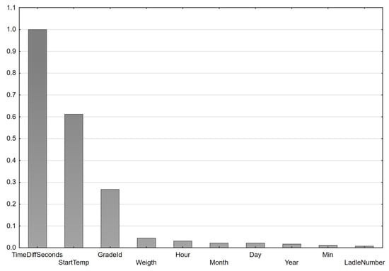
Figure 13.
Importance of explanatory variables (predictors) in the CART model.
The value of the tests and the selection of predictors for divisions can be read directly from the tree (Figure 14a,b). Due to its size, the tree is presented in two parts. First, the left side of the tree (Figure 14a), and then the right side (Figure 14b). The whole structure, as a map of the nodes, is visible in Figure 11, as we can see, the list ID22 was repeated; ID24 and ID25 were easier model reading.
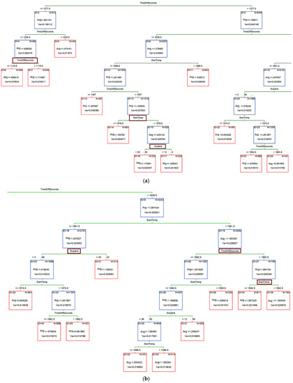
Figure 14.
The CART tree for the CoolingRate dependent variable presented in two fragments (a) the left side of the tree and (b) the right side. The individual nodes are marked in blue, while the final leaves are marked in red.
We can see that the training set was divided according to the cooling time; the lower the cooling time, the higher the cooling rate. The highest is 1.9 even for the leaf ID6 with the cooling time below 1119 s. For some steel grades, the cooling coefficient was even lower than 1.
The presented model explains well the nature of the variability of the cooling rate and the most important factors affecting it. However, if we want to increase the precision of the prediction, we should use models with continuous characteristics, such as linear regression or neural networks.
The significance of CART models lies mainly in their potential to represent complex relationships in a dataset. They allow both the researcher and the technologists to understand and visualize the impact of individual parameters on the output variable. They indicate not only which factors are important, but also how they affect the temperature drop, thereby allowing for better planning of the process and modeling the phenomenon, also using other algorithms.
4. Regression and Artificial Neural Networks
Linear regression (LR) and artificial neural networks (ANN) were applied to model the considered process as comparable machine learning techniques. Both approaches are well known, therefore their description is omitted in this paper. Detailed information on ANNs can be found in Bishop [11], Hagan et al. [12], and Haykin [13], while information on LR can be found in Seber and Lee [14], Kung [15], and Joshi [16].
MATLAB R2021a software was employed for all computations. The creation and training of the artificial neural networks (ANNs) were carried out using the Deep Learning Toolbox, while the Optimization Toolbox was employed to perform gradient optimization of the cost function for linear regression. In both scenarios, the primary objective of the model was to estimate the steel temperature following a designated time interval. This estimation was based on several parameters: the steel type (GradeID), the initial temperature after heating (StartTemp), the cooling duration (TimeDiff), and the weight of the steel (Weight). Additionally, the cooling rate was calculated using the temperature difference and the cooling time. After undergoing filtering, the collected dataset comprised over 73 hundreds of records. These records correspond to 81 distinct steel grades. Regrettably, there was a substantial discrepancy in the number of records for individual steel grades, as evidenced in Figure 15.
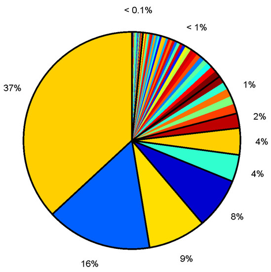
Figure 15.
The quantity of entries for specific steel grades. Seven types of steel (with IDs: 1, 10, 3, 52, 5, 19, and 30) were represented by more than 2% of the data.
The prevalent steel type (with ID 1) was related to 37% of data, i.e., over 30 hundreds of records. Five types of steel were represented by about 1% of data. Less than 1% of data were related to 34 types of steel and less than 1‰ was related to 35 types of steel. Despite these pronounced variations in the record counts, the initial model training demonstrated that the number of steel types included in the training set did not significantly influence the model’s accuracy. As a result, computations were carried out for all 81 steel types.
4.1. Linear Regression
The value predicted by linear regression model is computed using the hypothesis in the following form:
where: is the model’s parameter vector, x is the feature vector (input of the model with an added element ), and n = 4 which signifies the number of features.
Model training involves determining the optimal values of the parameter vector , which minimizes the cost function:
where: m is the number of training data points, is the model’s prediction for the ith training point, and is the actual training value for the ith data point.
The pivotal factor in achieving model accuracy lies in the selection of features (elements of the input vector). The inclusion of the four aforementioned features was determined after conducting an importance analysis. However, the limited number of features results in a simple model that may be incapable of grasping the complex relationships embedded within the training data. This scenario is known as underfitting or the high bias problem. To mitigate underfitting, it is necessary to introduce new features into the hypothesis. These new features can encompass entirely novel data or, more commonly, constitute combinations of existing data (features).
In this study, additional features were defined as higher powers (up to the 4th) of the already chosen inputs and all conceivable products formed from them. Consequently, the feature count was expanded to , and each new feature was defined as follows:
where: , and .
Conversely, incorporating supplementary features into the hypothesis can potentially lead to a model that is excessively intricate and learns the underlying data relationships in a rote manner. This scenario is referred to as overfitting or the high variance problem. Overfitting can be identified by comparing errors calculated for both the training and the testing (validation) sets. If the training error is minimal while the validation error is notably higher, an issue of high variance is present. To counteract the risk of overfitting, a regularization term was introduced to the optimized cost function:
where —is the regularization parameter and —represents the number of features.
The training was performed several times for different values of the regularization parameter, and then the best LR predictor was chosen.
4.2. Artificial Neural Network
The second model was constructed using artificial neural networks. An ANN is an information processing system comprising a specified count of individual components known as artificial neurons (ANs). Each artificial neuron (as illustrated in Figure 16) possesses varying numbers of inputs and produces a single output.
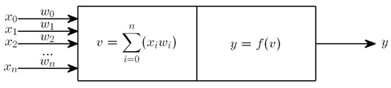
Figure 16.
Artificial neuron.
The AN’s output is calculated through a two-step process. Initially, each input value xi is multiplied by a synaptic weight coefficient wi. In the subsequent step, the resultant sum is used as the input to an activation function f, yielding the neuron’s output y. While the activation function remains constant, the weight parameters undergo adjustments during the neuron’s training phase. The training objective is to determine the weight parameter values that enable the neuron to respond effectively to input values and replicate the modelled phenomenon. However, due to the limited approximation capabilities of a single neuron, artificial neural networks are employed in practice. These ANNs consist of a specified number of interconnected neurons, organized into three layers: input, hidden, and output, respectively. A commonly used type of neural network is the multi layer perceptron (MLP) feed-forward network (as shown in Figure 17).
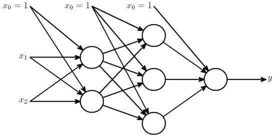
Figure 17.
A representative example of an artificial neural network includes two input nodes, one output node, and a hidden layer comprising three artificial neurons.
The number of neurons in the input (output) layer is contingent upon the count of input (output) values, while the determination of the hidden layers is typically based on experiential factors, often involving no more than two hidden layers for addressing nonlinear problems. In most scenarios, the output layer contains one neuron that corresponds to the output value of the modeled phenomenon. The design of a neural network involves the following three stages: (1) defining the architecture of the artificial neural network (network topology, activation functions), (2) training the ANN, and (3) testing the ANN.
The chief characteristic of an ANN lies in its learning capability, which consequently grants it a robust approximation capacity for multivariate nonlinear functions. This attribute renders it a valuable tool for modeling intricate processes, along with delivering a high degree of computational efficiency.
Typically, the output layer comprises a solitary neuron that corresponds to the anticipated prediction. In the context of an artificial neural network, the inclusion of new features is generally not mandatory. As such, the input vector was only composed of the four features. However, the network’s structure, specifically the topology (including the number of hidden layers and neurons within them), significantly influences model accuracy. Regrettably, there exist no definitive rules for determining the optimal count of hidden layers and neurons. Consequently, the training of the ANN was conducted 100 times, and the best network configuration—consisting of a single hidden layer with 19 neurons—was selected.
To compare the trained models, two errors were calculated:
where: m represents the number of testing data points, denotes the model’s prediction for each testing point, stands for the actual testing value, and signifies the mean testing value.
The obtained errors for all trained models are presented in Table 3.
Table 3.
Assessment of models’ predictions to the real values.
5. Summary
The presented research report aims to use statistical data analysis and machine learning models such as regression trees, linear regression, and neural networks in the development of predictive models applicable in predicting the cooling rate in the process of continuous casting of steel. Machine learning models have shown sufficient accuracy in successfully replacing numerical models that do not allow for the real-time prediction of the process when results are needed on-line as the ladle moves down the production line. Machine learning models do not require assumptions about ranges or the distributions of input variables. However, they are usually limited to a set of training sets and do not fulfil their role in extrapolating ranges. This is their main limitation. Models can learn dependencies, but only in the ranges represented by the training data. In addition, decision trees, which work by dividing the set into partitions, are by definition a spliced model, so that although the results are quantitative, they are the average in a group of similar records and are discrete, which makes their precision very limited (as seen in the scatter plot in Figure 12). Neural networks, on the other hand, have a non-linear continuous output but their nature makes it impossible to trace the learned relationship, they are a black box and do not allow the phenomenon to be studied. Therefore, the use of all these methods together gives the greatest benefit to both the analyst and the end user. Cooling rate prediction aims to improve the material preparation process for CST devices. Predicting the cooling rate allows the temperature to be accurately determined over time, which in turn makes it possible to precisely determine the temperature at which the ladle should leave the LMS stand without overheating. All of this is performed to improve the processes.
On the basis of the developed models, in particular neural networks and CART trees, predictive modules were implemented in the monitoring system of the electric steel plant, which was developed for the needs of the CMC steelworks in Zawiercie. This system, based on production data, is designed to support the entire steel production process, from the EAF furnace to the CC station. To achieve this, it is necessary to control data from each stage of the process. Data from production systems as well as ladle location data (from cameras) are analyzed to determine the location of each ladle and its status, including temperature, at all times. We are most interested in the LMS because it lasts the longest and gives the most control over the energy used. The models have been verified during ongoing production and their effectiveness has been highly rated. The results of the analyses based on the monitoring system’s indications have not yet been published, however, problems related to the system’s implementation have already been the subject of publication [17]. A full evaluation will be possible when the system has been in operation for a longer period of time and will certainly be the subject of a separate publication.
The use of modern measurement techniques, smart sensors, IoT in data transfer, cloud computing in the implementation of predictive models, numerical models in calculating the values of decision variables, and finally machine learning in the continuous improvement of metamodels is all in line with the idea of Industry 4.0 [18] and is aimed at implementing the idea of cyber-physical systems in the future [19]. This concept suggests monitoring technological processes by comparing ongoing operations with anticipated outcomes, which are concurrently calculated using a virtual model. This approach aims to uphold the anticipated quality level. In essence, it involves continuous prediction of ongoing operation results, coupled with automatic control and self-governing decision making within cyber-physical systems [20].
The authors present models that provide a satisfactory credibility in the forecasts and allow for the implementation of a continuous on-line parameter forecast within a time that allows for decision making during the process.
Author Contributions
Conceptualization, K.R.; Data curation, M.P.; Formal analysis, K.R., Ł.S. and M.P.; Funding acquisition, Ł.R.; Investigation, K.R., Ł.S. and M.P.; Methodology, K.R., Ł.S. and M.P.; Project administration, Ł.R.; Supervision, Ł.R.; Validation, Ł.R.; Writing—original draft, K.R., Ł.S. and M.P.; Writing—review and editing, K.R., Ł.S. and M.P. All authors have read and agreed to the published version of the manuscript.
Funding
This research was funded by financial support from the Intelligent Development Operational Program: POIR.01.01.01-00-0996/19.
Data Availability Statement
Restrictions apply to the availability of these data. Data was obtained from CMC Poland. Data sharing is not applicable to this article.
Conflicts of Interest
The authors declare no conflict of interest. The funders had no role in the design of the study; in the collection, analyses, or interpretation of data; in the writing of the manuscript; or in the decision to publish the results.
References
- Hay, T.; Visuri, V.-V.; Aula, M.; Echterhof, T. A Review of Mathematical Process Models for the Electric Arc Furnace Process. Steel Res. Int. 2020, 3, 2000395. [Google Scholar] [CrossRef]
- You, D.; Michelic, S.C.; Bernhard, C. Modeling of Ladle Refining Process Considering Mixing and Chemical Reaction. Steel Res. Int. 2020, 91, 2000045. [Google Scholar] [CrossRef]
- Zappulla, M.L.S.; Cho, S.-M.; Koric, S.; Lee, H.-J.; Kim, S.H.; Thomas, B.G. Multiphysics modeling of continuous casting of stainless steel. J. Mater. Process. Technol. 2020, 278, 116469. [Google Scholar] [CrossRef]
- Santos, M.F.; Moreira, M.H.; Campos, M.G.G.; Pelissari, P.I.B.G.B.; Angélico, R.A.; Sako, E.Y.; Sinnema, S.; Pandolfelli, V.C. Enhanced numerical tool to evaluate steel ladle thermal losses. Ceram. Int. 2018, 44, 12831–12840. [Google Scholar] [CrossRef]
- Kusiak, J.; Sztangret, Ł.; Pietrzyk, M. Effective strategies of metamodelling of industrial metallurgical processes. Adv. Eng. Softw. 2015, 89, 90–97. [Google Scholar] [CrossRef]
- Tan, P.-N.; Steinbach, M.; Kumar, V. Introduction to Data Mining; Addison-Wesley: Boston, MA, USA, 2005. [Google Scholar]
- Rokach, L.; Maimon, O. Top-Down Induction of Decision Trees Classifiers—A Survey. IEEE Trans. Syst. Man Cybern. Part C Appl. Rev. 2005, 35, 476–487. [Google Scholar] [CrossRef]
- Barros, R.C.; de Carvalho, A.; Freitas, A.A. Automatic Design of Decision-Tree Induction Algorithms; Springer International Publishing: Berlin/Heidelberg, Germany, 2015. [Google Scholar]
- Regulski, K.; Wilk-Kołodziejczyk, D.; Kluska-Nawarecka, S.; Szymczak, T.; Gumienny, G.; Jaśkowiec, K. Multistage discretization and clustering in multivariable classification of the impact of alloying elements on properties of hypoeutectic silumin. Arch. Civ. Mech. Eng. 2019, 19, 114–126. [Google Scholar] [CrossRef]
- Balamurugan, M.; Kannan, S. Performance analysis of cart and C5.0 using sampling techniques. In Proceedings of the IEEE International Conference on Advances in Computer Applications (ICACA), Coimbatore, India, 24–24 October 2016. [Google Scholar] [CrossRef]
- Bishop, C.M. Neural Networks for Pattern Recognition; Oxford University Press: Oxford, UK, 1995. [Google Scholar]
- Hagan, M.T.; Demuth, H.B.; Beale, M.H. Neural Network Design; PWS Pub. Co., Ltd.: London, UK, 1996. [Google Scholar]
- Haykin, S. Neural Networks: A Comprehensive Foundation; Prentice Hall: Hoboken, NJ, USA, 1999. [Google Scholar]
- Seber, G.A.F.; Lee, A.J. Linear Regression Analysis; Wiley-InterScience: Hoboken, NJ, USA, 2003. [Google Scholar]
- Kung, S.Y. Kernel Methods and Machine Learning; Cambridge University Press: Cambridge, UK, 2014. [Google Scholar]
- Joshi, A.V. Machine Learning and Artificial Intelligence; Springer Nature: Cham, Switzerland, 2020. [Google Scholar]
- Hajder, P.; Opaliński, A.; Pernach, M.; Sztangret, Ł.; Regulski, K.; Bzowski, K.; Piwowarczyk, M.; Rauch, Ł. Cyber-physical System Supporting the Production Technology of Steel Mill Products Based on Ladle Furnace Tracking and Sensor Networks. In Computational Science–ICCS 2023; Lecture Notes in Computer Science; Springer: Cham, Switzerland, 2023; p. 10477. [Google Scholar] [CrossRef]
- Gajdzik, B.; Wolniak, R. Framework for activities in the steel industry in popularizing the idea of industry 4.0. J. Open Innov. Technol. Mark. Complex. 2022, 8, 133. [Google Scholar] [CrossRef]
- Zhang, C.J.; Zhang, Y.C.; Han, Y. Industrial cyber-physical system driven intelligent prediction model for converter end carbon content in steelmaking plants. J. Ind. Inf. Integr. 2022, 28, 100356. [Google Scholar] [CrossRef]
- Graupner, Y.; Weckenborg, C.; Spengler, T.S. Designing the technological transformation toward sustainable steelmaking: A framework to provide decision support to industrial practitioners. Procedia CIRP 2022, 105, 706–711. [Google Scholar] [CrossRef]
Disclaimer/Publisher’s Note: The statements, opinions and data contained in all publications are solely those of the individual author(s) and contributor(s) and not of MDPI and/or the editor(s). MDPI and/or the editor(s) disclaim responsibility for any injury to people or property resulting from any ideas, methods, instructions or products referred to in the content. |
© 2023 by the authors. Licensee MDPI, Basel, Switzerland. This article is an open access article distributed under the terms and conditions of the Creative Commons Attribution (CC BY) license (https://creativecommons.org/licenses/by/4.0/).