Cold Spray Process for Co-Deposition of Copper and Aluminum Particles

Abstract

Mixed-particle spraying has been applied to various aspects of industrial cold spraying for a long time. Due to the complexity of mixed-particle simulations, most studies only consider dozens of particles when considering particle collisions. This paper combines computational fluid dynamics and a discrete element method to analyze the entire trajectories of mixed particles. With simulations involving over one hundred thousand particles, we accurately tracked the three-dimensional positions and velocities of each particle, effectively visualizing their journey from feeder to substrate. By comparing the particles’ velocities to their critical velocities, we could directly assess the deposition efficiency, achieving a comprehensive and accurate simulation of the complete cold spray process. The numerical model was validated using a multi-experimental analysis. The particle distribution and deposition area from the numerical model matched well with the experimental data. It was found that the mutual collision of copper and aluminum particles increased the number of copper particles, surpassing the critical velocity in the mixed powder by 24.2%. When copper particles and aluminum particles collided, the displacement of aluminum particles was more than three times that of copper particles in the direction perpendicular to the jet. This collision caused the aluminum particles to be more dispersed.

1. Introduction

In the cold spraying process (CSP), the powder particles are accelerated by a supersonic gas jet and heated to a temperature lower than the melting point of the material before impacting the substrate, resulting in the formation of a metallurgically bonded coating of particles in the solid state [1]. CSP does not require high temperatures to melt particles and, therefore, avoids some of the problems associated with thermal spraying methods, such as evaporation, melting [2], high-temperature oxidation of particles [3], and gas release [4]. These problems can affect the chemical composition, microstructure, and properties of the coating. Cold spray technology also reduces or eliminates residual stresses and crystallization in the coating, thereby improving the stability and durability of the coating [5,6,7,8]. Mixed-particle spraying has been applied to various aspects of industrial cold spraying for a long time. The common components of the mixed phase include Al [9], Cu [10], Fe [11], Ti [12], Ni [13], and W [14]. This technology has an immense range of industrial applications in designing and manufacturing metal materials with different physical properties [15,16]. In these application scenarios, the properties of metal particles used in the spraying process, such as size, shape, velocity, and distribution, have important effects on the performance and function of the materials [17]. Therefore, the study of the velocity and distribution of metal particle mixtures during the spraying process is of great importance to industry and research.

The initial studies on cold spraying of mixed-metal powders were based on experiments. Kang et al. [14] deposited agglomerated tungsten/copper composite powders onto a mild steel substrate and obtained a composite coating with good performance. Subsequently, Zhao et al. [9] used CSP to spray mixed-metal particles and obtained a metal composite coating. In addition, Price et al. [10] mixed copper and aluminum powders in a 1:1 volume ratio and sprayed them onto a copper substrate using CSP, and observed the creation of an intermetallic compound layer at the interface. Che et al. [17] combined tin with copper and zinc powders, and used a low-pressure system to perform cold spraying, and found that the deposition efficiency could be significantly increased by adding a second metal powder. Although these experimental studies were not very accurate, they made great contributions to the research on spraying of mixed particles.

With the gradual improvement in the understanding of mixed powder coatings, in order to pursue a higher deposition efficiency, these mixed powder spraying experiments have put forward higher requirements for obtaining the state of the sprayed particles. If the dynamic behavior of the particles can be obtained more accurately, this information can be used to prepare coatings with better effects. Therefore, it is necessary to obtain more accurately particles’ dynamic behavior. Now, more and more studies have adopted numerical methods to simulate the cold spraying process. For example, Karimi et al. [18] used computational fluid dynamics (CFD) and non-axial powder feeding nozzle model to study the trajectory and distribution of particles in the airflow. Liebersbach et al. [19] used user-defined functions (UDFs) created in Ansys-Fluent to record the velocities of the particles and compare them with the critical velocity. Faizan-Ur-Rab et al. [20] used CFD to calculate the trajectory of a titanium particle jet inside and outside the nozzle. But these studies only considered the influence of the airflow on particles, and ignored the influence of the particles on each other. How to introduce particle-phase interactions in cold spraying simulations is the problem.

To accurately characterize the profile of the cold spray coating on the substrate surface and establish a correlation between CFD results and the actual coating, Zhu et al. [21] used the spatial distribution of the particles’ positions and velocities predicted by CFD. For more accurate simulations, Leitz et al. [22] integrated discrete unit particle descriptions with a CFD method based on the discrete element method (DEM) to simulate the airflow. By leveraging existing theoretical and simulation methods, their proposed theory and simulation techniques enabled the acquisition of accurate information on the velocities of the particles. This approach improved understanding of the cold spray and provided insights into the influences of different factors on particle behavior. Krull et al. [23] used the DEM to simulate particle collisions and performed meshing with two different resolutions to obtain the specific state of the particles after collision. Due to the limitations of experimental studies, modeling the flow field and particles in flight with coupled CFD and DEM could lead to more logical and trustworthy results for the study of particles’ distribution and their acceleration behavior.

In order to model the particles’ interactions with each other, many researchers use software such as Abaqus v6.4 to model the particles [24,25]. This method can better reflect the collision of the particles when the number of particles is only a few or dozens, but in the whole cold spraying process, the number of sprayed particles can reach at least hundreds of thousands. At this time, analyzing individual particles may not be useful enough. We should pay more attention to the deposition of the particles as a whole. Therefore, it is necessary to couple the CFD and DEM techniques to model the whole spraying process. This method can simulate far more particles than Abaqus, and also consider the actual situation of each particle separately. It can take into account both the airflow effect on the particles and the interaction between the particles. It can simulate an immense number of particles at the same time and treat each particle as an independent element. This methodology strikes a balance between efficiency and precision, providing a more realistic depiction of the whole spraying process. In this study, we applied the CFD-DEM approach to analyze the entire trajectories of mixed particles. With simulations involving over one hundred thousand particles, we accurately tracked the three-dimensional positions and velocities of the particles, effectively visualizing their journey from feeder to substrate. By comparing the particles’ velocities to their critical velocities, we could directly assess the deposition efficiency, achieving a comprehensive and accurate simulation of the whole spraying process.

2. Experiment Method

2.1. Cold Spray

The supersonic spraying process is carried out with a supersonic low-pressure cold sprayer which compresses the gas through a scaled Laval nozzle to produce a supersonic air stream. The powder is introduced axially into the supersonic air stream, creating a two-phase flow that accelerates before impacting the substrate in its solid state. The particles deposit on the substrate’s surface after undergoing significant plastic deformation. As shown in Figure 1, the cold spray apparatus (Beijing Techny Materials and Technology Co., Ltd., Beijing, China) was applied. Compressed air was selected as the carrier gas and the system pressure was set to 0.7 MPa.

Commercial Cu and Al powders were initially mixed in a 1:1 volume ratio, SS316L was chosen as the substrate material for cold spray coating due to its excellent mechanical properties and weldability [26], which facilitate the assessment of the coating-to-substrate morphology and the optimization of the cold spray parameters and outcomes. Air was employed as the powder feed gas during cold spraying, with a powder temperature of 500 °C. At a feed rate of 0.524 g/s and an intake pressure of 0.7 MPa, the powder was added. In the experiment, there was a 20 mm distance between the nozzle and the substrate, which was considered by Samareh et al. [27] to be the optimum spraying distance for low-pressure cold spraying.

The respective micromorphologies of the copper and aluminum powders and their particle size analyses are shown in Figure 2. The spherical particles range in size from 10 to 50 μm, which was shown to be the most suitable range for spraying by Schmidt et al. [28]. With an oxygen tester, it was found that the powders’ oxygen content was less than 0.01 wt.% (RO316; LECO, MI). The relationship between the cumulative mass fraction and particle size was found utilizing a laser diffraction particle size meter (MASTERSIZER 3000; Malvern Instruments Ltd., Malveron, UK), and is plotted in Figure 2b,d.

In this study, mixed particles were deposited onto the substrate at 500 °C and accelerated by a Laval nozzle at 0.7 MPa. The cross-section of the composite coating was analyzed using an Oxford Xplore energy dispersive spectrometer (EDS) and a German Zeiss GeminiSEM 300 scanning electron microscope (SEM), and the results are presented in Section 4.1. The substrate surface was roughened using sand blasting prior to deposition to increase surface roughness and reduce surface tension to improve the coating’s adhesion and wear resistance. The substrate surface was preheated to reduce the temperature difference and stress between the substrate and the coating to avoid cracking or peeling of the coating.

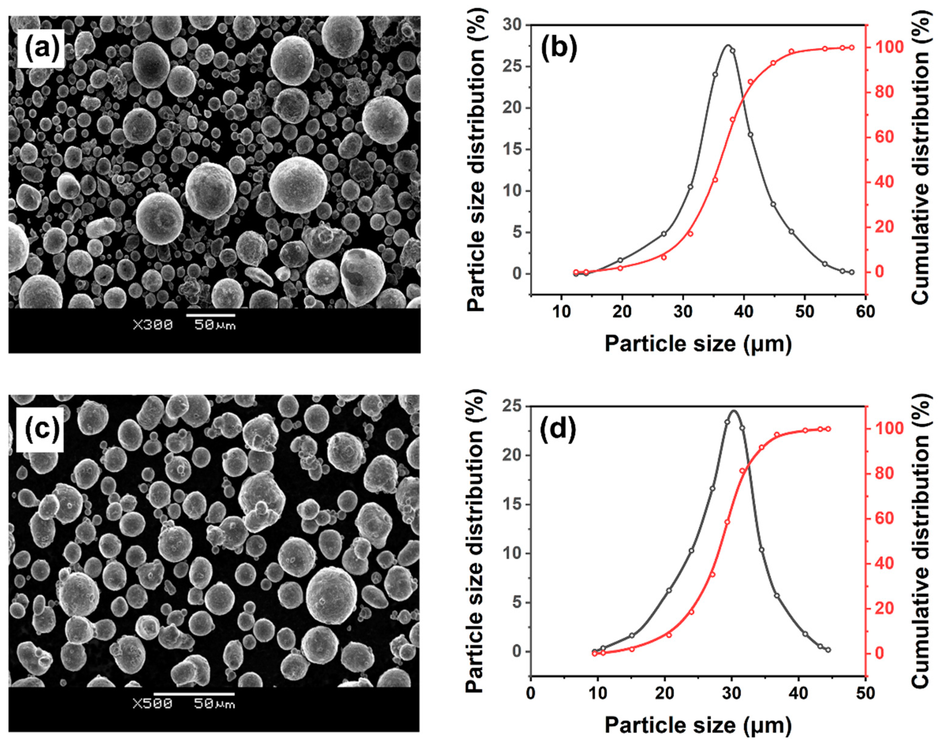
2.2. Particle Distribution Analysis

In the past, cold spraying validation usually used a high-speed camera or particle image velocimetry (PIV) for model verification [29,30]. The high-speed camera can measure the velocity of individual particles, while PIV can measure the velocity field in the fluid. In this study, there were tens of thousands of particles in the DEM simulation, so the accuracy and efficiency of the high-speed camera were not satisfactory, and PIV could only infer the particle velocity from the flow field velocity, which was contrary to what this study required. Therefore, in order to verify the model accurately, this paper used SEM + EDS verification, chemical composition verification, and critical velocity verification, and ensured the accuracy of the whole experiment through three aspects of verification. The verification results are given in Section 4.1.

A special explanation is needed in this section for the chemical composition verification method. A spectrophotometric method was used to determine the amount of copper and aluminum in the samples. After the light passed through the sample and a portion was absorbed, the absorbance value was calculated and then converted to the sample’s concentration. The absorbance value of a sample is inversely proportional to its concentration [31].

To ensure the accuracy of the spectrophotometric measurement, the absorbance should be controlled to be between 0.1 and 0.8. Therefore, a series of copper standard solutions need to be prepared and a working curve needs to be plotted, and then compared with the sample solutions obtained from the experiment. The specific steps are as follows:

First, prepare the copper standard stock solution. Weigh 1 g of copper and put it in a 400 mL beaker containing 20 mL of water and 10 mL of nitric acid, cover it with a watch glass, and wait for the copper to dissolve completely. Then, place the beaker on a water bath and evaporate the solution until crystals start to precipitate. Next, dissolve the crystals with water and transfer the solution to a 1000 mL volumetric flask, add water to the mark, and mix well. This is the copper standard stock solution, containing 1 mg of copper per 1 mL.

Next, prepare the copper standard solution. Transfer 5.00 mL of the copper standard stock solution to a 500 mL volumetric flask, add water to the mark, and mix well. This is the copper standard solution, containing 0.01 mg of copper per 1 mL.

Finally, prepare a set of copper solutions with different concentrations and measure their absorbance. Transfer 0 mL, 0.50 mL, 1.00 mL, 2.00 mL, 3.00 mL, 4.00 mL, 5.00 mL, and 6.00 mL of the copper standard solution to a set of 250 mL beakers, and add 20 mL of water and 3 mL of hydrochloric acid to each beaker, and mix well. There is no need to adjust the pH of the solutions, just use the reagent blank solution as the reference. On the spectrophotometer, select the wavelength of 460.0 nm and measure the absorbance of each solution. Then, plot the working curve with the mass concentration of copper (mg/mL) as the horizontal axis and the absorbance as the vertical axis. The working curve was created and linearly fitted as a function of $y=0.07534x+0.00101$ in Figure 3.

As illustrated in Figure 4, two regions were chosen for testing purposes. Region 1 was 1 cm in width and 1.8 cm in height, and region 2 was 1 cm in width and 0.4 cm in height. The central axes of the two regions were designated as a and b, respectively, with a spacing of 2 cm between them.

These specific areas were selected for further analysis in this study. The specific method is as follows: two parts of the region are wire-cut and placed in a 250 mL beaker, adding 5 mL of water and 15 mL of hydrochloric acid (4.2.3). After the test material is completely dissolved, add 2 mL of nitric acid, heat and boil for 2 min~3 min, drive off the nitrogen oxides (blank evaporation to about 2 mL), wash the walls of the cup with a small amount of water, and cool to room temperature. Filter using slow filter paper (if clear and bright cannot be filtered). Wash the filter paper and residue 8 to 10 times with hot hydrochloric acid (4.2.3). Collect the filtrate and washings in a 400 mL beaker. If there is a large amount of residue, place the filter paper with the residue in a platinum crucible, dry, and ashyllate completely at 550 °C (do not burn), and cool. Add 2 mL of sulfuric acid (4.2.5) and 5 mL of hydrofluoric acid (4.2.1), and add nitric acid (4.2.4) drop by drop until the solution is clear. Heat and evaporate until sulfuric acid fumes appear, burn at 700 °C for 10 min (not exceeding 700 °C), then cool. Add as little hydrochloric acid as possible and a few milliliters of water, heat to dissolve the precipitate completely (filter if cloudy), and combine the solution with the main test solution. Add 8 mL of ammonium citrate solution, and then 5 mL of hydroxylamine hydrochloride solution to the test solution, mix well, then add 5 mL of ethanol solution of neocuproine. Throw in a small piece of Congo red test paper, use ammonia to adjust until the Congo red test paper turns red, change to pH paper, and then continue to carefully adjust to a pH value of about 4.5. Transfer the test solution to a 250 mL dispensing funnel to make a volume of about 60 mL–70 mL. Use a spectrophotometer at 460.0 nm wavelength. Measure the absorbance of the solution at 460.0 nm.

To determine the percentage of copper and aluminum content, the absorbance of the blank solution was subtracted from the absorbance of the sample and the corresponding copper content was determined using the working curve.

3. Numerical Method

3.1. Coupling Process

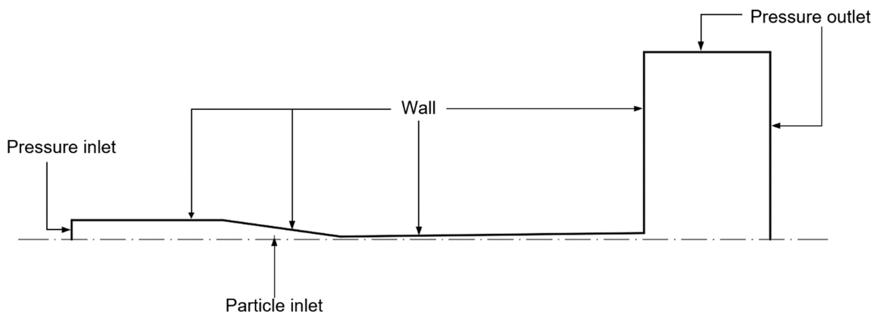
The CFD-DFM coupling was the transient bi-directional data transfer process. As shown in Figure 5, the coupled simulation was based on Fluent’s UFD. Fluent was used to calculate the flow field for one time step and then initiate the EDEM for the same time iteration. The particle position, motion, volume, and temperature data were transferred to Fluent by the coupling interface, and it is at this point that the interaction between the particles and the fluid is calculated by the Fluent v15.0. The action on the fluid was applied to the fluid through the momentum source phase, while the action of the particles was applied to the particles in the form of particle volume forces. As the coupling between the EDEM and Fluent calculations has a time step difference, the time step needs to be set small enough to ignore the time misalignment effect. The Euler–Euler method is used to calculate the gas–solid two-phase flow.

The supersonic spraying process is carried out with a supersonic low-pressure cold sprayer which compresses gas through a scaled Laval nozzle to produce a supersonic air stream. The powder is introduced axially into the supersonic air stream, creating a two-phase flow that accelerates before impacting the substrate in its solid state. The particles deposit on the substrate’s surface after undergoing significant plastic deformation.

3.2. CFD Model

3.2.1. Gas Flow

The $RNG k-\epsilon$ model is better in fast-strain flows. Compressed air is used as the processing gas, which is assumed to be an ideal and compressible gas with a specific heat capacity of 1006.43 J/kg K and a molecular mass of 28.966. The continuity, momentum, and energy conservation equations in their Reynolds-averaged general conservation forms are used to consider and calculate the effect of turbulence on the flow field, as shown in Equations (1)–(3). Obviously, compared with the standard k–ɛ model, the $RNG k-\epsilon$ model can improve the accuracy of the rapid-strain flow [32]. The realizable k–ɛ model does not take into account the effect of low-Reynolds-number viscosity, such as the flow near the wall. Therefore, in this physical problem, the accuracy of solving the turbulent eddy is the most important factor, so the gas flow in the Laval nozzle is considered to be the $RNG k-\epsilon$ turbulent model [33], as shown in Equations (4) and (5). This turbulent model can accurately simulate the flow field of both high- and low-velocity gas flow [34].

Mass:

$$\frac{\partial \left(\rho {\mu }_i\right)}{\partial x_i}=0$$

(1)

Momentum:

$$\frac{\partial }{\partial x_j}\left(\rho {\mu }_i{\mu }_j\right)=\frac{\partial }{\partial x_j}\left[{\mu }_{\mathrm{eff}}\left(\frac{\partial {\mu }_j}{\partial x_j}+\frac{\partial u_i}{\partial x_i}\right)-\frac{2}{3}{\mu }_{\mathrm{eff}}\frac{\partial u_k}{\partial x_k}\right]-\frac{\partial p}{\partial x_i}$$

(2)

Energy:

$$\frac{\partial }{\partial x_j}\left(\rho {\mu }_i{\mu }_j\right)+\frac{\partial p}{\partial x_i}=\frac{\partial }{\partial x_j}\left[{\mu }_{\mathrm{eff}}\left(\frac{\partial {\mu }_j}{\partial x_j}+\frac{\partial u_i}{\partial x_i}\right)-\frac{2}{3}{\mu }_{\mathrm{eff}}\frac{\partial u_k}{\partial x_k}\right]$$

(3)

Turbulence energy:

$$\frac{\partial }{\partial x_i}\left(\rho u_{i}k\right)=\frac{\partial }{\partial x_i}\left[\left({\alpha }_k{\mu }_{\mathrm{eff}}\frac{\partial k}{\partial x_i}\right)\right]+{\mu }_i{S}^2-\rho \epsilon$$

(4)

Turbulence energy dissipation:

$$\frac{\partial }{\partial x_i}\left(\rho u_i\epsilon \right)=\frac{\partial }{\partial x_i}\left[\left({\alpha }_{\epsilon }{\mu }_{\mathrm{eff} }\frac{\partial \epsilon }{\partial x_i}\right)\right]+C_{1\epsilon }\frac{\epsilon }{k}{\mu }_i{S}^2-C_{2\epsilon }\rho \frac{{\epsilon }^2}{k}-R$$

(5)

For compressible flow, the state equation of the ideal gas can be written as Equation (6).

$$\frac{p}{\rho }=RT$$

(6)

k is the k equation coefficient, $\epsilon$ is the turbulence energy dissipation coefficient, $\rho$ is the gas density, and ${\mu }_{\mathrm{eff}}$ is the effective viscosity coefficient. The coefficients ${\alpha }_T$, ${\alpha }_k$, and ${\alpha }_{\epsilon }$ are the reciprocal of the effective Prandtl of energy k and $\epsilon$ equation, respectively. $S$ is the mean-velocity strain-rate tensor coefficient. The constants $C_{\mu }$, $C_{1\epsilon }$, and $C_{2\epsilon }$ have values of 0.085, 1.42, and 1.68, respectively. R is the gas constant, T is temperature.

3.2.2. The Model of CFD

The boundary conditions are displayed in Figure 6 and

Table 1. Boundary conditions.

	Pressure, MPa	Temperature, K
Inlet	0.7	773.15
Wall	…	Adiabatic
Outlet	0.101	293.15

. The propellant gas utilized in the CSP operated at a temperature of 773.15 K and a pressure of 0.7 MPa. The particles were introduced into the gas stream radially, taking advantage of the Venturi effect at the converging section located 171 mm away from the nozzle throat. In this study, the computational domain for cold spray was obtained by rotating the cross-section shown in Figure 6 around the x-axis. The results are shown in Figure 7; the specific data of the cross-section are given in

Table 2. Geometric parameters of the model.

Geometric Parameter	Length, mm
Length of diverging section	141
Nozzle inlet diameter	13
Nozzle exit diameter	3
Length of converging section	55
Throat diameter	1.35

. In addition, an outer area in the form of a cylinder was included outside the nozzle with a radius of 90 mm and an outermost distance of 50 mm from the nozzle outlet. The effect of the stability of the air supply on the supersonic flow was ignored to simplify the numerical model. For the outlet located in the external zone, a temperature of 293.15 K and a pressure of 0.1 MPa were specified. The nozzle wall was treated as a smooth and immovable boundary, with no heat transfer occurring. The remaining areas of the computational domain were defined as non-reflective boundaries.

The nozzle is a converging–diverging Laval nozzle and its exact dimensions are shown in Table 2. To ensure an accurate simulation of the cold spray process, a hexahedral cell structure was employed to create the structural mesh. The mesh generation was performed using ANSYS ICEM 15.0, as illustrated in Figure 7. The mesh near the nozzle throat, the area near the wall, and the free jet area was refined to capture the flow property changes due to the flow compressibility [35,36]. The convergence criterion was set to be 10⁻⁶ and the time step was set to be 0.0001 s, which is small enough to capture the transient behavior of the flow and powder particles, and also large enough to ensure a reasonable computational time. The mesh sensitivity analysis was performed by increasing the computational cells and refining the mesh until the nozzle’s axial velocity change from the previous refinement was below 1%. A total cell number of about 1,260,000 was adopted in this simulation work.

The independence of the calculation result from the mesh density was checked. Total cell numbers of about 600,000, 2,000,000, and 2,500,000 were checked. Under the condition of 600,000 cells, the calculation could not reach convergence due to the poor quality of the mesh. While under the 2,000,000- and 2,500,000-cell scale, the results showed no evidence of difference from the 1,260,000-cell scale.

The Fluent and EDEM meshes were different, but they did not interfere with each other when coupled. The typical geometry of a cold spray model in the EDEM calculation domain is illustrated in Figure 8. The converging and dispersing Laval nozzle with a high air pressure and smooth surface was contained in the cold spray multivariate model. It was surrounded by a cylindrical zone 360 mm long and 400 mm in diameter. To ensure the efficiency and stability of the calculation, the grid size in EDEM is generally set to twice the radius of the smaller particles. In this study, it was 0.02 mm. The grid size has nothing to do with the solution accuracy [23]. The model was solved numerically by EDEM using the Eulerian method. For the calculations, 20% of the Rayleigh time step was chosen as the time step. In addition, the simulation grid was configured to be twice the particle radius. These settings were implemented to speed up the calculation while maintaining an acceptable level of accuracy in the simulation results.

To investigate the impact of dissimilar particle mixing on particle trajectories outside the nozzle, a virtual circular substrate of 6 mm radius was placed 20 mm away from the nozzle outlet. The distance of 20 mm has previously been determined to be the most suitable distance for spraying [27].

As shown in Figure 9, during the spray simulation, the virtual substrate in EDEM does not collide with the particles, but is able to record the exact position and the exact velocity of the particles at that moment. The particle positions and properties passing through the virtual substrate are recorded and further processed. This approach is accurate and efficient enough that it can record data for very large numbers of particles while ensuring sufficient simulation speed.

3.3. CFD Model

The discrete element method uses a soft-sphere model to track the motion of each particle. The method computes each particle as a discrete individual, allows for particle collisions, and considers multiple particle collisions. Cleary et al. [37] employed the DEM method to solve the discrete problem with excellent results. The influence between the particles and the fluid, as well as among the particles themselves, can be effectively modeled using the discrete unit control equations of the DEM, which are mainly divided into the particle-phase control equation and the continuous phase–particle phase coupling equation.

3.3.1. Particle-Phase Control Equations

The core of DEM calculations is the analysis of interactions and feedbacks between solid phases in gas–solid systems. The particle contact model was selected for collision analyses between solid phases in which the particles were subject to four main forces: particle gravity, pressure gradient forces, particle–particle collision forces, and gas tracer forces on the particles. The equation of motion of the particles can be expressed as

$$m_i\frac{d{V}_i}{dt}=F_{d,i}+m_{i}g+\Sigma \left(F_{n,ij}+F_{t,ij}\right)-V_p\nabla p$$

(7)

$$I_i\frac{d{\omega }_i}{dt}=\Sigma T_{t,ij}$$

(8)

in this equation, $m_i$ indicates particle mass, while $F_{t,ij}$ and $F_{n,ij}$ denote the tangential and normal forces exerted on particle i by particle j, respectively. The moment generated by the tangential stress of the particle collision is represented by the variable $T_i$. Furthermore, ${\omega }_i$, $I_i$, and $V_i$ represent the angular velocity of particle i, rotational inertia, and translational velocity, respectively. $V_p$ and ${\nabla }_p$ represent the volume of the particle and the pressure gradient at the particle, respectively. For inter-particle forces ($F_{n,ij}$, $F_{t,ij}$), a linear model is used [38]. These variables are crucial in describing the motion and interactions of particles within the cold spray process. The wall is considered to be a stationary particle and is calculated using equations similar to those used for inter-particle collisions. With the above forces and moments, the velocity, position of the particle, velocity, and rotational velocity can be expressed as

$$V_i=V_{i,0}+\frac{d{V}_i}{dt}\Delta t$$

(9)

$${\omega }_i={\omega }_{i,0}+\frac{d{\omega }_i}{dt}\Delta t$$

(10)

$$xy{z}_i=xy{z}_{i,0}+V_i\Delta t$$

(11)

Models of particles of the same shape and different sizes were created using EDEM with reference to the SEM images and particle size distribution maps obtained using photography, as shown in Figure 10. The particles created generally matched the actual particles in terms of particle size distribution, dimensions, and surface smoothness, with yellow representing copper powder and silver-gray representing aluminum powder. The specific factors for the aluminum and copper particles are shown in

Table 3. Spray parameters.

Particle Material	Poisson’s Ratio	Solids Density	Modulus of Rigidity	Young’s Modulus
Cu	0.34	8960 kg/m3	4.63 × 1010 Pa	1.241 × 1011 Pa
Al	0.33	2710 kg/m3	2.62 × 1010 Pa	6.969 × 1010 Pa

, with the Poisson’s ratio and shear modulus being two key properties when performing DEM simulations [39].

3.3.2. Continuous-Phase Control Equation

The continuous-phase governing equations adopt the two-fluid model (model A) based on local averaging and considering the fluid–solid coupling effect. The following are the momentum equation and continuity equation:

$$\frac{\partial (\epsilon {\rho }_f)}{\partial t}+\nabla \cdot (\epsilon {\rho }_f{u}_f)=0$$

(12)

$$\frac{\partial (\epsilon {\rho }_f{u}_f)}{\partial t}+\nabla \cdot (\epsilon {\rho }_f{u}_f{u}_f)=-\epsilon \nabla p+\nabla \cdot (\epsilon \overline{\overline{{\tau }_f}})+S_{fp}+\epsilon {\rho }_{f}g$$

(13)

in the equation, $S_{fp}$ represents the fluid–solid coupling term. To increase the computational stability, the control Equations (12) and (13) are reorganized ($S_m$ and $S_c$ are the origin terms for the momentum equation and continuity equation after reorganization):

Continuity equation:

$$\frac{\partial {\rho }_f}{\partial t}+\nabla \cdot ({\rho }_f{u}_f)\frac{{\rho }_f}{\epsilon }(\frac{\partial \epsilon }{\partial t}+u_f\cdot \nabla \epsilon )=0$$

(14)

or

$$\frac{\partial {\rho }_f}{\partial t}+\nabla \cdot ({\rho }_f{u}_f)=S_c$$

(15)

among

$$S_c=-\frac{{\rho }_f}{\epsilon }(\frac{\partial \epsilon }{\partial t}+u_f\cdot \nabla \epsilon )$$

(16)

Momentum equation:

$$\epsilon \frac{\partial }{\partial t}\left({\rho }_f{u}_f\right)+\epsilon \nabla \cdot \left({\rho }_f{u}_f{u}_f\right)+{\rho }_f{u}_f\left(\frac{\partial \epsilon }{\partial t}+u_f\cdot \nabla \epsilon \right)=-\epsilon \nabla p+\nabla \cdot \left(\epsilon \overline{\overline{{\tau }_f}}\right)+S_f+\epsilon {\rho }_{f}g$$

(17)

among

$$S_m=\frac{S_{fp}}{\epsilon }-\frac{{\rho }_{f}g}{\epsilon }\left(\frac{\partial \epsilon }{\partial t}+u_f\cdot \nabla \epsilon \right)+\frac{\overline{\tau }\cdot \nabla \epsilon }{\epsilon }$$

(18)

3.3.3. Continuous-Phase Particle Coupling

The continuous-phase particle forces in this study included both traction and pressure gradient forces, which are provided in Equation (7). For the traction force, the algorithm is based on the coupling term in the gas-phase equation of the two-fluid model extended to the particle model, which in turn acts on the particle phase. The momentum exchange source term in the fluid equation of motion is expressed as

$$S_{fp}=\beta (u-v)$$

(19)

The interphase momentum exchange coefficient $\beta$ is

$$\left\{\begin{array}{cc}\beta =150\frac{{(1-\epsilon )}^2}{\epsilon }\frac{{\mu }_g}{d_p^2}+1.75(1-\epsilon )\frac{{\rho }_g}{d_p}|u-v|& \epsilon <0.8\\ \beta =\frac{3}{4}{C}_{d0}\frac{\epsilon (1-\epsilon )}{d_p}{\rho }_f|u-v|{\epsilon }^{-2.65}& \epsilon \ge 0.8\end{array}\right.$$

The particles’ Reynolds numbers in the particle population are

$$C_d=\left\{\begin{array}{cc}\frac{24}{\mathrm{Re}}\left[1+0.15{(\mathrm{Re})}^{0.687}\right]& Re<1000\\ 0.44& \mathrm{Re}\ge 1000\end{array}\right.$$

The Reynolds numbers of particles in the particle group are

$$\mathrm{Re}=\frac{\epsilon {\rho }_f|u-v|d_p}{{\mu }_f}$$

(20)

In Equation (19), the interphase momentum exchange coefficient $\beta$ and the particle Reynolds number formula, $\epsilon$ and $\nu$ are the average values in the grid.

After solving for the flow field, the tractive force on a single particle according to Newton’s third law is

$$F_d=\frac{V_P{\beta }_k}{1-{\epsilon }_k}(u_k-v_k)$$

(21)

${\epsilon }_k$ and ${\beta }_k$ represent the local porosity and local momentum exchange coefficient of particle k, respectively; $u_k$ is the virtual continuous-phase velocity at the particle k’s center of mass.

4. Results and Discussion

4.1. Numerical Validation of Models

4.1.1. SEM + EDS Verification

Particles of aluminum and copper were deposited onto a substrate made of SS316L to create the composite coating, which shows that Cu and Al particles underwent deformation and mechanical bonding under high-speed impact, forming a functional composite coating with some properties of Cu and Al coatings. In the process of forming this composite coating, due to the adiabatic shear instability effect, local materials softened, resulting in a metal jet phenomenon. A metal jet refers to the effect of metal with local thermal softening producing similar viscous material flow phenomena in the process of bonding with the substrate, making the flowing Cu and Al metals bond with each other. The SEM image of the coating-substrate interface is shown in Figure 11.

To further analyze the composition and structure of the composite coating, we performed EDS line scanning on the cut section of the composite coating, and quantitatively analyzed the proportion of each element from the center to the outside of the section. Figure 12 shows the results of the EDS line scan, which reflects the distribution of mixed particles from the center to both sides of the coating. The results show that from the center to the outside, the proportion of Cu particles gradually decreases, while that of Al particles gradually increases. This trend is consistent with the numerical analysis prediction in Section 4.2, and also verifies the accuracy of the numerical model. Since quantitative measurements of EDS line scans are inherently not very accurate, it is acceptable that there is a mismatch between experiment and simulation.

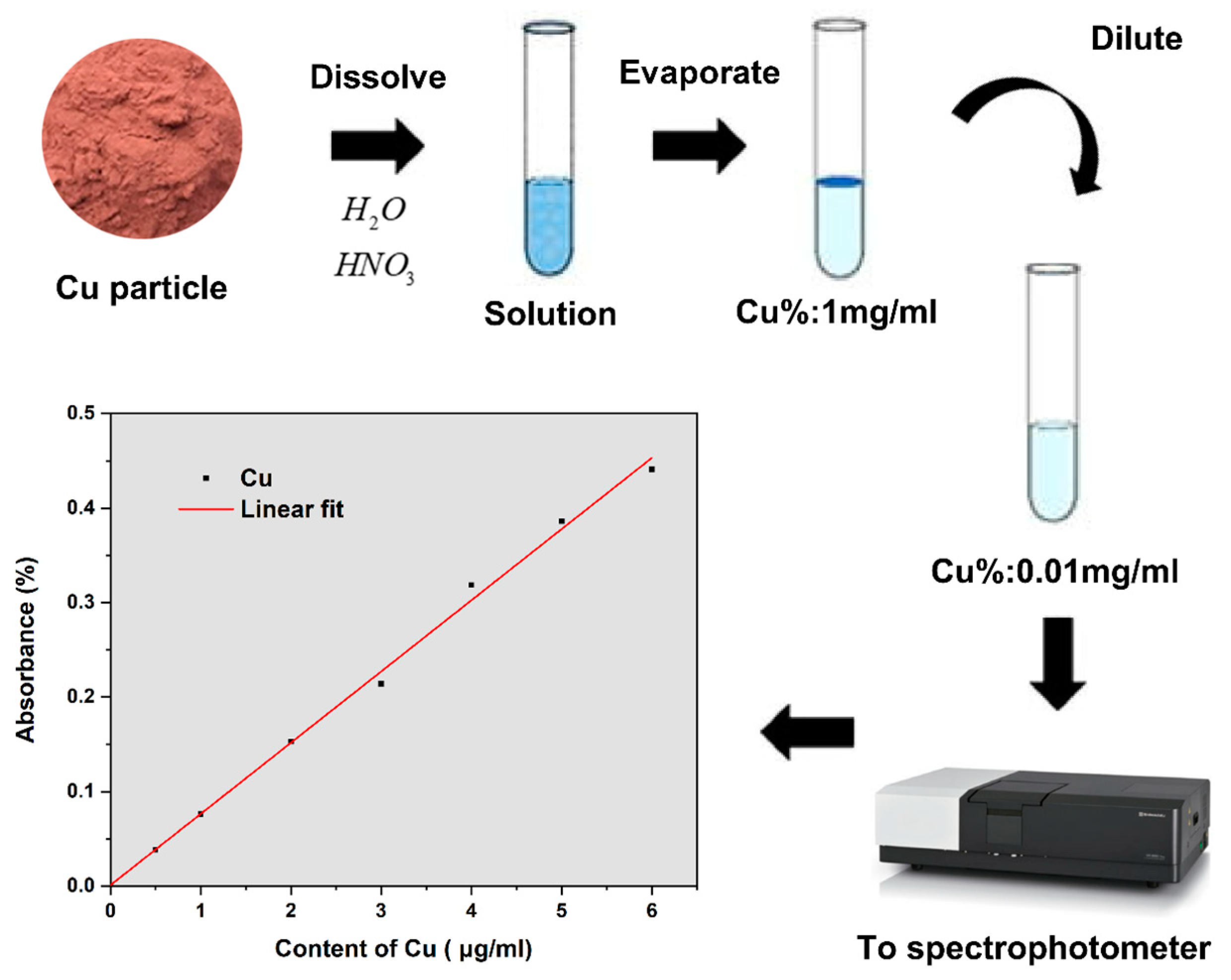
4.1.2. Chemical Composition Verification

As the EDS line scan does not accurately quantify the percentages of copper and aluminum mass in the deposit, it is important to quantify the copper and aluminum percentages using chemical methods once the elemental composition of the deposit is known. The distribution of copper and aluminum particles on the substrate was tested indirectly using spectrophotometry as described in Section 2.2. The correctness of the numerical model can be verified by comparing the simulation results with the experimental results.

After purification and dilution of the sample, the absorbance of the solution in different regions was measured using a UV–visible spectrophotometer (UV-3600i-Plus). As shown in Figure 13, at a wavelength of 460 nm, the absorbance of the solution in the two regions of the spectrophotometer was 0.3981% and 0.2110%, respectively. The copper content in the solution and the percentage of copper in the two regions were calculated and are listed in

Table 4. Mass percentage of copper in the two sampling regions.

Results	Region 1	Region 2
Absorbance	0.3981	0.2110
Content of copper (μg/mL)	5.2709	2.7873
Experimentally measured mass percentage (%)	54.175 ± 3.274% (95%)	30.046 ± 2.892% (95%)
Numerical predations of mass percentage (%)	54.261	32.592

. Based on the uncertainty analysis, the mass percentages of copper in region 1 and region 2 were 54.175 ± 3.274% (95%) and 30.046 ± 2.892% (95%), respectively. In the simulation, these data were 62.787% and 45.792%, respectively. But when we removed the copper particles with axial velocities below the critical velocity in the simulation [28,40], the mass percentages of copper particles in the two regions in the simulation were 54.261% and 32.592%, respectively. The simulation data and the experimental data were basically consistent. The predicted copper mass percentage at the edge was slightly larger than the experimental measurement result. The numerical models demonstrated by Assadi et al. [41] and Schmidt et al. [42] achieved similar results.

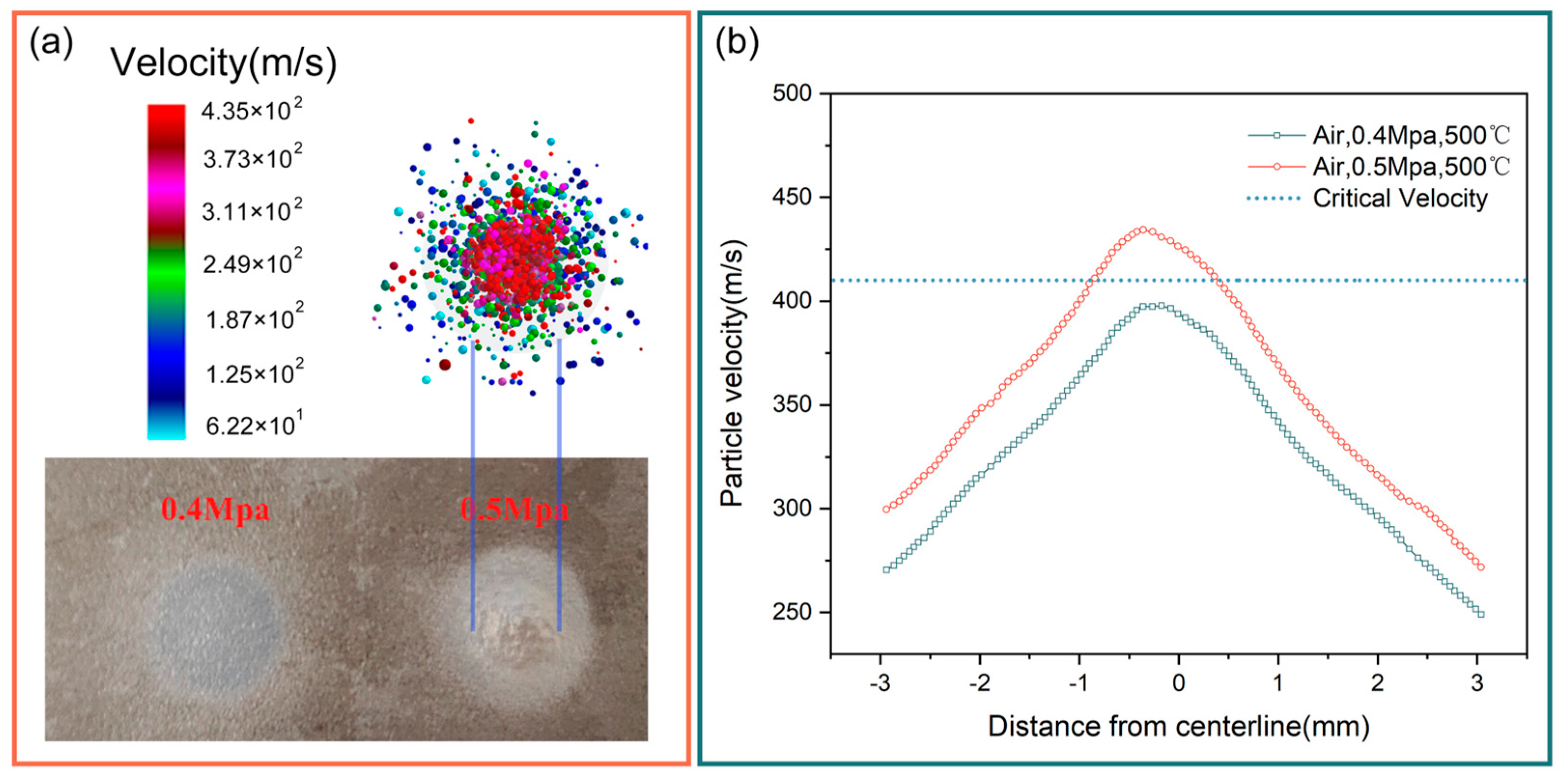
4.1.3. Critical Velocity Verification

According to previous research [43], only particles with a velocity above a critical threshold can be deposited on the substrate. So the critical velocity can be regarded as the lower limit of the deposition velocity. Schmidt et al. [28] measured the critical velocity of spherical pure aluminum particles as 400–420 m/s.

To measure the critical velocity roughly through experiment, the aluminum particles were sprayed vertically for 3 s at five different nozzle inlet pressures: from 0.1 MPa to 0.5 MPa, increased by 0.1 MPa each time. The simulated results showed that some of the aluminum particles were deposited to the substrate at 0.5 MPa. Only some of the particles reached the critical velocity. When the pressure was 0.4 MPa, no deposition was found on the substrate. This indicated that the critical velocity of the aluminum particles at 500 °C was between 0.4 MPa and 0.5 MPa. The simulated particle velocity at 0.5 MPa is shown in Figure 14. The maximum velocity was 435 m/s and the particles near the center exceeded the critical velocity of 400–420 m/s. The deposition area determined through experimentation was identical to the critical velocity range in the simulated velocity plot, Figure 14a. At 0.4 MPa, the maximum velocity of 397 m/s was below the critical velocity, so no particles were deposited on the substrate.

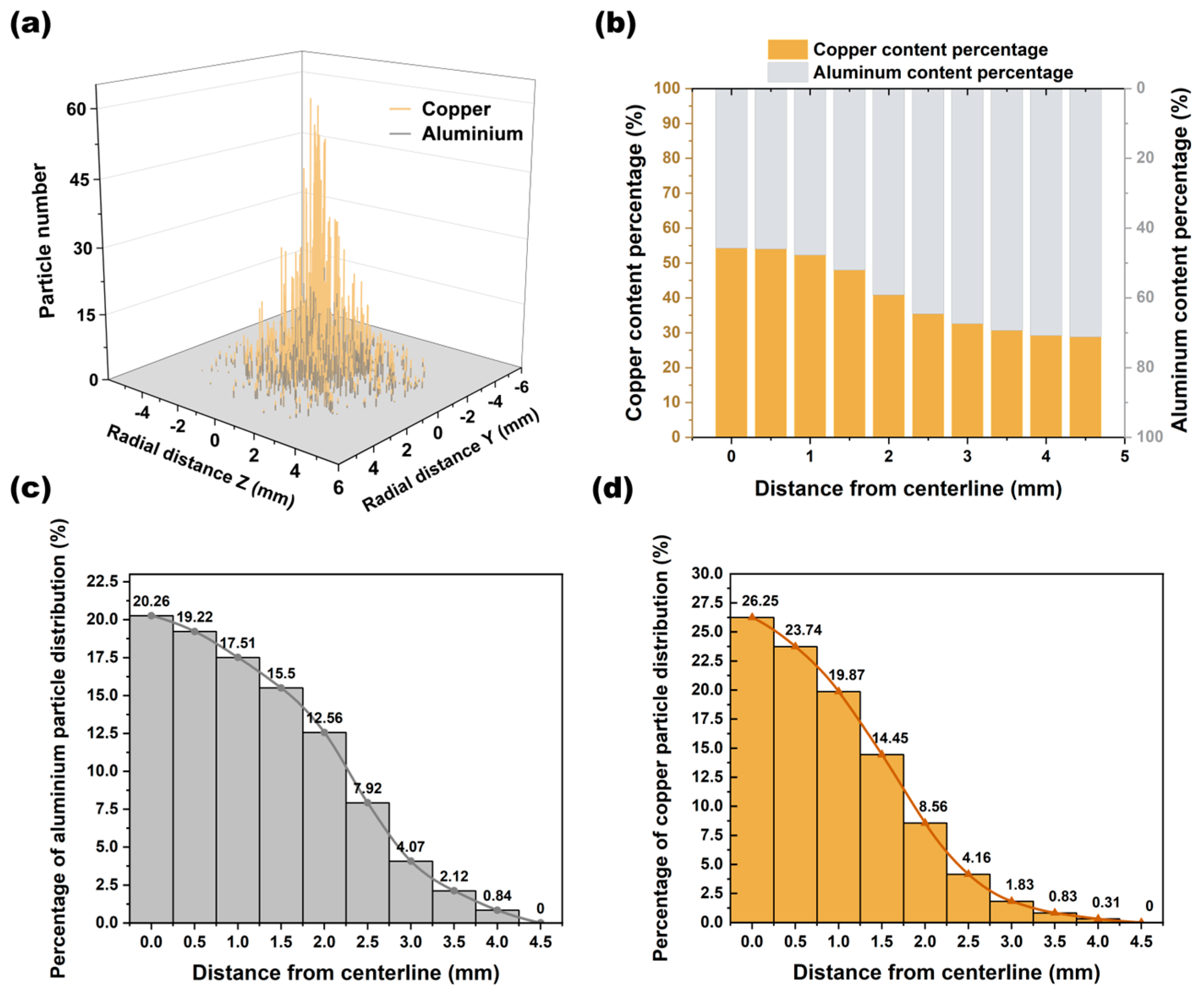
4.2. Particle Distribution

When you have an axial nozzle, most particles should move near the centerline. For spraying of the same kind of particles, this may be true. But when the sprayed object is a mixed-metal powder, everything is different. When the mixed-metal powder is sprayed, due to the different densities of the two powders, under the same spraying conditions, the forces along and perpendicular to the velocity direction on the two powders are completely different, making the system more chaotic during spraying. The different distributions of the two particles are caused by many factors acting together, which can be classified into two aspects: particle collision and flow field interference. The first is the collision of particles. In fact, in the simulation, we found a lot of particle collisions. When copper and aluminum particles collide in the direction perpendicular to the jet, the displacement of aluminum particles is more than three times that of copper particles. This kind of collision naturally makes aluminum particles more divergent. Secondly, the existence of the flow field itself will make copper and aluminum particles show different divergence and convergence states, which will be discussed in detail below.

The particle distribution inside and outside the nozzle when the simulation approached steady state is presented in Figure 15. It is clear that more particles are concentrated towards the center of the nozzle. Inside the Laval nozzle, the particles and the surrounding air have a velocity difference. This velocity difference creates a velocity gradient in the fluid, perpendicular to the particle motion. Consequently, there is a force in the nozzle in the low- to high-velocity direction [44]. This force is the Safmann lift. The equation for the Saffman lift force is as follows:

$$F_s=1.61d_p^2{\left({\rho }_g{\mu }_g\right)}^{1/2}\left({\mu }_g-{\mu }_p\right){\left|d{u}_g/dy\right|}^{1/2}$$

(22)

in this equation, $d$ indicates the particle diameter, ${\rho }_p$ represents the particle density, ${\rho }_g$ is the fluid density, $u$ indicates the hydrodynamic viscosity, while $u_p$, $u_g$, and $u_s$ denote the particle velocity, fluid velocity, and slip velocity (fluid–particle), respectively.

As the particles leave the Laval nozzle, the aluminum particles have a lower density than the copper particles, making them more susceptible to uneven shock-wave interference. As a result, the aluminum particles are more dispersed than the copper particles when they hit the substrate.

During the spray simulation, the particle positions and properties passing through the virtual substrate were recorded and further processed. The number of particles at different positions in the substrate when copper and aluminum particles were mixed and sprayed is shown in Figure 16a, where yellow indicates copper powder and gray indicates aluminum powder. Most of the particles were concentrated inside a circle with a radius of 3 mm. The volume share of the copper and aluminum particles from the center to the outside is given in Figure 16b. The percentage of aluminum particles increases towards the outer side, which proves that the aluminum particles were more divergent than the copper particles outside the nozzle. The distribution curves of copper and aluminum are shown in Figure 16c and Figure 16d, respectively. The copper powder had a higher possibility of falling into the central region than the aluminum powder.

Due to the pressure difference between the Laval nozzle exit and the surrounding environment, an expansion wave is initially generated. After multiple reflections at the jet boundary, a shock wave was formed, as shown in Figure 17. The two waves in the jet exhibited periodicity [45], which led to periodic fluctuations in the gas velocity, as evidenced by a sharp increase in the flow velocity followed by a rapid decrease [46].

After the particles left the nozzle, under the action of the shock wave, the outward dispersion continued. Unstable airflow produced a force component perpendicular to the particles so that the particles could not follow the straight line of motion. The magnitude of the interference is dependent on the volume of the mixed particles. Specifically, larger particles tend to exert a greater interference force. When the copper powder and aluminum powder volume was the same, the copper powder was less susceptible to airflow disturbances than the aluminum powder due to the density difference. On the other hand, as the velocity and acceleration of the copper and aluminum particles were different, collisions between the particles were inevitable when the feed rate increased. When collisions occurred among the particles, the aluminum powder was more likely to deviate from its own velocity direction. Therefore, the aluminum powder was more divergent outside the Laval nozzle than the copper powder. Periodic excitation played a key role in the dispersion of the aluminum powder.

As shown in Figure 18, this paper studied the spraying process of mixed copper and aluminum particles under the conditions of 500 °C temperature and 2 MPa inlet pressure. The figure shows the different velocities of the particles with different colors on the virtual substrate. (The particles are magnified for observation). The figure shows that the particle velocity decreases radially from the center to the outside during the spraying process. Also, the figure displays the distribution of the positions of the copper and aluminum particles at the moment of impact on the substrate, with the color yellow for the copper particles and silver-gray for the aluminum particles. It can be seen that the copper particles are more densely packed in the center of the spray compared to the aluminum particles.

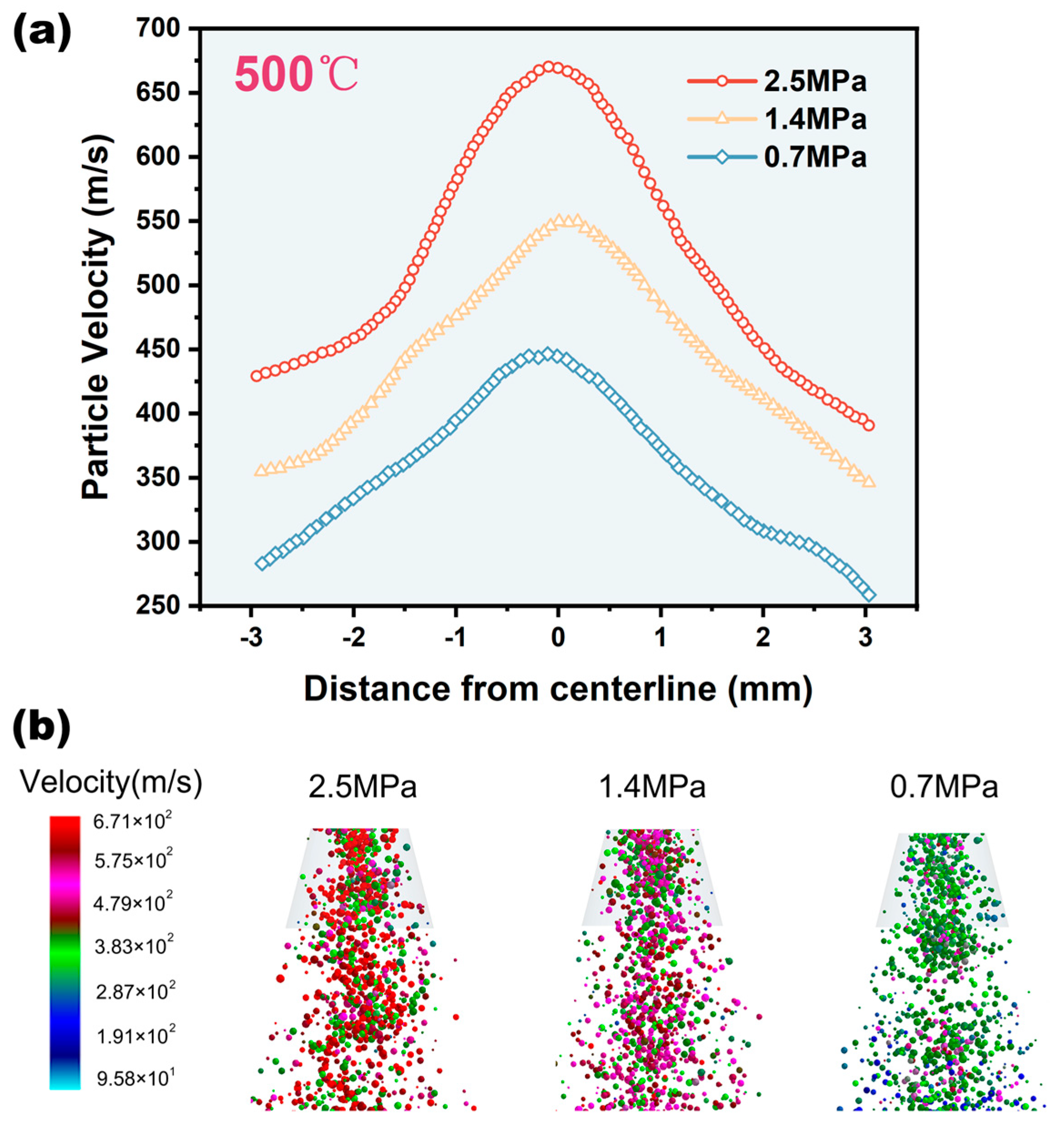
4.3. Influence of Inlet Pressure on Mixed Particles

The average velocities of the mixed copper and aluminum particles accelerated by the airflow are shown in Figure 19a,b. It can be observed that the air velocity curve oscillates at the nozzle outlet and is consistently higher than the particle velocity. However, as the particles travel further from the nozzle, their velocity gradually increases and eventually exceeds the air velocity. Notably, the oscillation of the airflow has a minimal impact on the particle velocity.

In this paper, the axial velocity distribution of mixed particles was studied by increasing the inlet air pressure while keeping the temperature constant in the simulation. According to Figure 20, each point in the figure represents the average axial velocity of 50 adjacent particles in the simulation. It can be observed that the velocity of mixed particles increases with the rise in inlet air pressure, and reaches the maximum value of 605 m/s at 2.5 MPa. On the other hand, the farther the particles are from the spraying center, the lower the axial velocity, and the more difficult it is to deposit on the substrate. This means that raising the air pressure is an effective way to increase the velocity of mixed particles, as in the case of pure particles. The velocity distribution along the nozzle axis shows some asymmetry [47]. This is mainly because in DEM, each particle has its own characteristics, so there are no particles with exactly the same velocity; even if 50 particles at the same position are averaged, there is still a velocity difference.

4.4. Influence of Temperature on Mixed Particles

The particle velocity distribution when increasing the temperature of the airflow and particles during the simulation while keeping the inlet air pressure constant is presented in Figure 21. Overall, the particle velocity slightly increased as the temperature rose from 500 °C to 700 °C. Once the temperature increases, the internal energy of the air also increases, leading to higher air kinetic energy. Consequently, the air velocity inside the nozzle increases. However, the average particle velocity increased by a maximum of only 29 m/s when the temperature increased by 200 °C.

Increasing the temperature had a more significant effect on enhancing the deposition efficiency of the mixed particles than increasing the air pressure, although the increase in temperature had a negligible effect on particle velocity. Of course, the gas temperature and particle temperature have to be increased at the same time in the experiment. According to a previous study, for every 100 °C increase in temperature, the particle critical velocity decreases by about 16 m/s. [48]. Figure 22 shows the percentage of particles exceeding the critical velocity at different air pressures and temperatures [28,40]. When the air pressure is elevated by 40%, the particles exceeding the critical velocity increase by 12.9%. Whereas, when the temperature is elevated by 40%, the number of particles exceeding the critical velocity is elevated by 20.9%. Obviously, when boosting the inlet air pressure and temperature by the same percentage, temperature has a greater effect on the deposition efficiency than inlet air pressure. However, higher temperatures also pose a risk of particle oxidation.

4.5. Deposition Profile and Efficiency

In this paper, an experimental comparison of the deposition morphologies of pure aluminum, pure copper, and mixed-particle sprays was carried out under the same process parameters. The cross-sectional profiles of the deposits are nearly triangular, as shown in Figure 23. The figure shows that the deposit height decreased and the deposit area increased with mixed spraying as the copper content in the aluminum powder increased. However, when all or most of the sprayed particles were copper particles, the area deposited on the substrate decreased instead. Furthermore, when the copper particles were sprayed alone, the deposits only extended as far as 2.18 mm from the center of the spray, whereas the aluminum particles extended as far as 2.35 mm when they were sprayed alone. More interestingly, when copper and aluminum particles were mixed, the deposits could extend as far as 2.65 mm from the center of the spray, which also suggests that the mixed particles were dispersed to a more peripheral area during the spraying process due to impacts and fluid action. In this study, mainly aluminum particles were dispersed. In other words, hybrid spraying makes it easier for lighter particles to be dispersed.

In order to investigate the reasons for the variation in deposition efficiency, SS316l was used as the substrate material in this paper and the deposits were wire-cut and weighed.

Table 5. Comparison of deposition efficiency.

Sample	Powder Weight (g)	Deposition Weight (g)	Deposition Efficiency (%)
Cu	3.368	0.739	21.932
Al	0.996	0.309	31.053
Cu + Al	2.244	0.713	31.774

shows the total sprayed powder mass, which is obtained by multiplying the powder feeding rate by the spraying time. The results show that the maximum deposition efficiency was achieved with the copper–aluminum mixture (1:1 volume ratio), which is similar to the deposition efficiency when aluminum particles were sprayed alone, but it also shows that the mixed powder spraying enables the deposition of copper particles that could not have been previously deposited In order to investigate the reason for this, the velocity data of copper and aluminum particles sprayed alone and in a mixture were collected during the simulation, with a total of 100,000 particles collected. The particles were sorted into velocity intervals and the data are exhibited in Figure 24. It can be observed that when copper and aluminum particles are sprayed together, the average velocity of the mixed powder is 26 m/s higher than the average velocity of the copper powder sprayed alone. The number of copper particles in the mixed powder exceeding the critical velocity [40] increases by 24.2%. Whereas, the number of aluminum particles exceeding the critical velocity [28] in the hybrid powder decreases by only 9.4%. Therefore, this increases the deposition efficiency of the mixture of copper and aluminum particles. It also shows that when the deposition efficiency of one powder is not satisfactory, the deposition efficiency can be improved by blending the powder with another lower-density powder for spraying.

5. Conclusions

In this paper, the whole cold spraying process was simulated comprehensively and accurately for the first time by coupling CFD and DEM. Hundreds of thousands of mixed particles in the CSP were considered individually, and the interactions between solid particles and airflow as well as the collisions between solid particles were added, and the three-dimensional position and velocity of each particle were accurately tracked. To validate the numerical model, multi-angle experimental analysis was also carried out. The main conclusions are as follows:

(1)

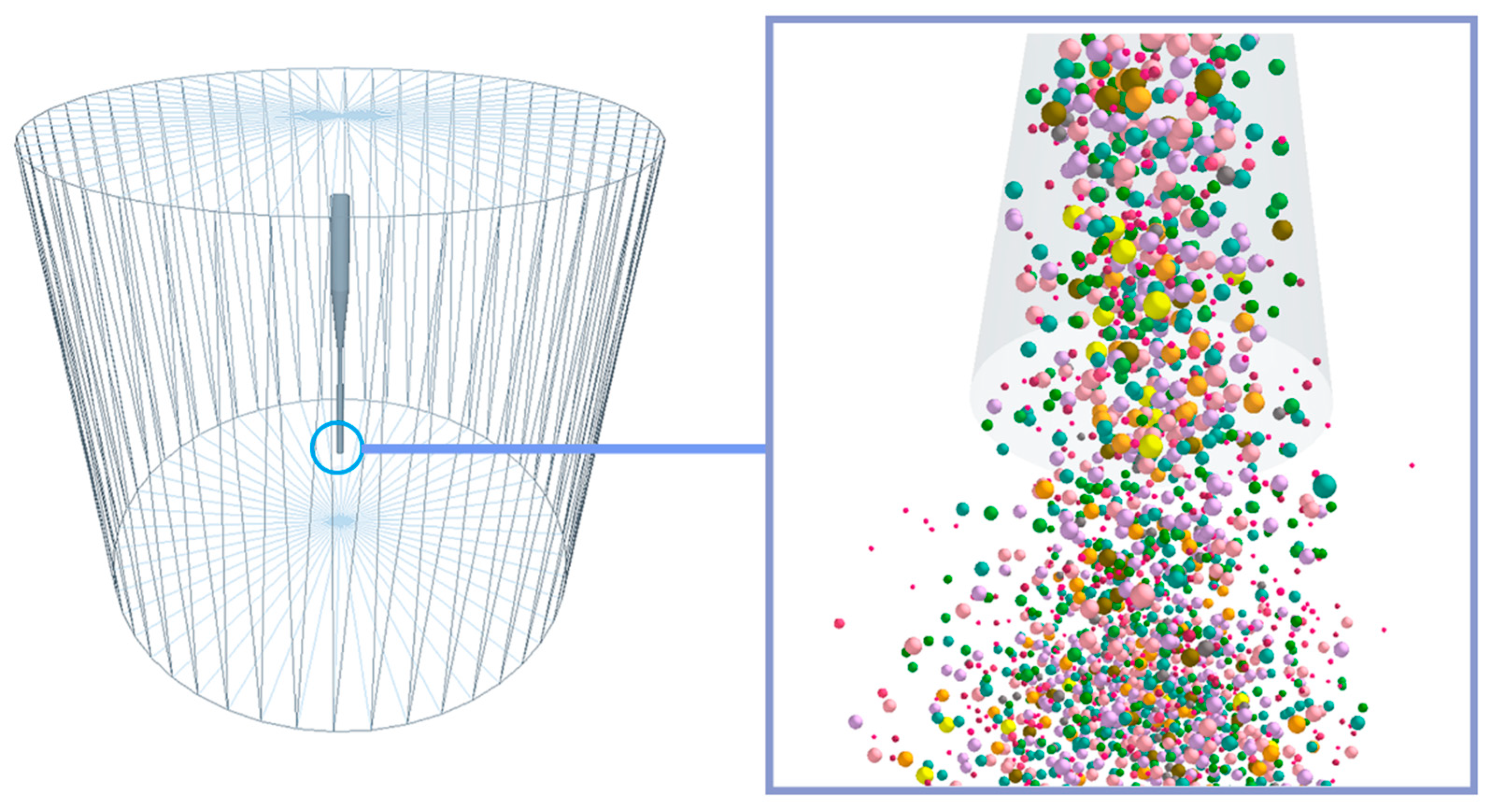
A large number of particle collisions were observed during spraying, and the mutual collisions of copper and aluminum particles increased the number of copper particles exceeding the critical velocity in the mixed powder by 24.2%. This indicates that when the deposition efficiency of one kind of powder is unsatisfactory, it can be improved by mixing it with another kind of powder with a lower density for spraying.

(2)

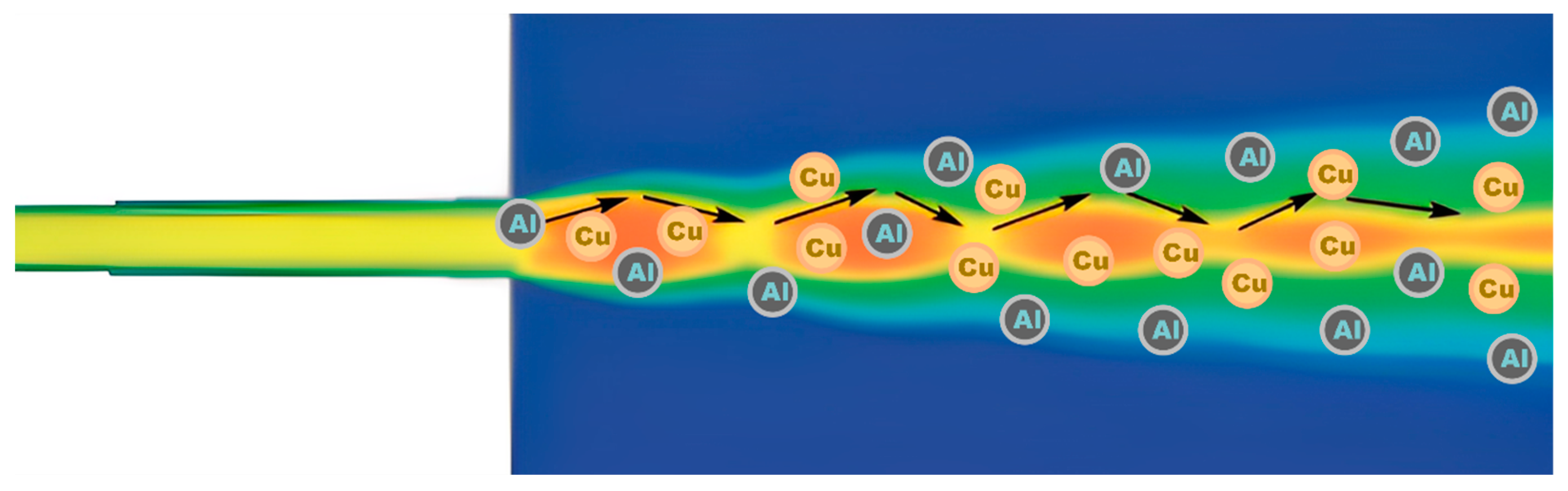
Mixed-metal spraying increased the disorder in the CSP. Due to the different densities of the copper and aluminum particles, when the powder feed rate increased, the collisions between particles were inevitable. When copper and aluminum particles collided in the direction perpendicular to the jet, the displacement of aluminum particles was more than three times that of copper particles. These collisions made aluminum particles more divergent. Secondly, the existence of the flow field itself made copper and aluminum particles show different divergence and convergence states.

(3)

Increasing the temperature and inlet pressure could improve the deposition efficiency of particles, and CFD-DEM revealed the principle more comprehensively. Increasing the inlet pressure could speed up particle velocity, while increasing temperature could reduce particle critical velocity.

(4)

In the case of mixed spraying, as the copper particle content in the aluminum powder increased, the height of the deposit decreased, and due to particle collision increases and fluid action, the area deposited on the substrate increased. However, when all or most of the sprayed particles were copper particles, collisions decreased and the fluid effects on particles tended to be similar, and the area deposited on the substrate decreased.

References

1. Assadi, H.; Kreye, H.P.D.; Gärtner, F.; Klassen, T. Cold spraying—A materials perspective. Acta Mater. 2016, 116, 382–407. [Google Scholar] [CrossRef]
2. Chavan, N.M.; Kiran, B.; Jyothirmayi, A.; Phani, P.S.; Sundararajan, G. The Corrosion Behavior of Cold Sprayed Zinc Coatings on Mild Steel Substrate. J. Therm. Spray Technol. 2013, 22, 463–470. [Google Scholar] [CrossRef]
3. Daroonparvar, M.; Bakhsheshi-Rad, H.R.; Saberi, A.; Razzaghi, M.; Kasar, A.K.; Ramakrishna, S.; Menezes, P.L.; Misra, M.; Ismail, A.F.; Sharif, S.; et al. Surface modification of magnesium alloys using thermal and solid-state cold spray processes: Challenges and latest progresses. J. Magnes. Alloys 2022, 10, 2025–2061. [Google Scholar] [CrossRef]
4. Rokni, M.R.; Nutt, S.R.; Widener, C.A.; Champagne, V.K.; Hrabe, R.H. Review of Relationship Between Particle Deformation, Coating Microstructure, and Properties in High-Pressure Cold Spray. J. Therm. Spray Technol. 2017, 26, 1308–1355. [Google Scholar] [CrossRef]
5. Zhang, Z.; Liu, Z.; Zhao, J.; Wang, B.; Cai, Y. Numerical analysis of residual stresses induced by cold spray fabricating cBN-reinforced Ni matrix composites. Surf. Coat. Technol. 2023, 467, 129672. [Google Scholar] [CrossRef]
6. Cui, L.; Fang, K.; Cao, J.; Hao, E.; Zhu, J.; Liu, G.; Hao, J. A practical method to improve mechanical and electrical properties of ADS copper prepared by cold spray additive manufacturing through powder pretreatment. J. Alloys Compd. 2023, 965, 171319. [Google Scholar] [CrossRef]
7. Huang, C.; List, A.; Wiehler, L.; Schulze, M.; Gärtner, F.; Klassen, T. Cold spray deposition of graded Al-SiC composites. Addit. Manuf. 2022, 59, 103116. [Google Scholar] [CrossRef]
8. Seng, D.H.L.; Zhang, Z.; Zhang, Z.-Q.; Meng, T.L.; Teo, S.L.; Tan, B.H.; Loi, Q.; Pan, J.; Ba, T. Impact of spray angle and particle velocity in cold sprayed IN718 coatings. Surf. Coat. Technol. 2023, 466, 129623. [Google Scholar] [CrossRef]
9. Zhao, Z.B.; Gillispie, B.A.; Smith, J.R. Coating deposition by the kinetic spray process. Surf. Coat. Technol. 2006, 200, 4746–4754. [Google Scholar] [CrossRef]
10. Price, T.S.; Shipway, P.H.; McCartney, D.G.; Calla, E.; Zhang, D. A Method for Characterizing the Degree of Inter-particle Bond Formation in Cold Sprayed Coatings. J. Therm. Spray Technol. 2007, 16, 566–570. [Google Scholar] [CrossRef]
11. Wang, H.; Li, C.-J.; Yang, G.; Li, C.-X. Cold spraying of Fe/Al powder mixture: Coating characteristics and influence of heat treatment on the phase structure. Appl. Surf. Sci. 2008, 255, 2538–2544. [Google Scholar] [CrossRef]
12. Novoselova, T.; Fox, P.; Morgan, R.; O’Neill, W. Experimental study of titanium/aluminium deposits produced by cold gas dynamic spray. Surf. Coat. Technol. 2006, 200, 2775–2783. [Google Scholar] [CrossRef]
13. Lee, H.Y.; Jung, S.H.; Lee, S.Y.; Ko, K.H. Alloying of cold-sprayed Al–Ni composite coatings by post-annealing. Appl. Surf. Sci. 2007, 253, 3496–3502. [Google Scholar] [CrossRef]
14. Kang, H.-K.; Kang, S.B. Tungsten/copper composite deposits produced by a cold spray. Scr. Mater. 2003, 49, 1169–1174. [Google Scholar] [CrossRef]
15. Aydin, H.; Alomair, M.; Wong, W.; Vo, P.; Yue, S. Cold Sprayability of Mixed Commercial Purity Ti Plus Ti6Al4V Metal Powders. J. Therm. Spray Technol. 2017, 26, 360–370. [Google Scholar] [CrossRef]
16. Che, H.; Chu, X.; Vo, P.; Yue, S. Cold spray of mixed metal powders on carbon fibre reinforced polymers. Surf. Coat. Technol. 2017, 329, 232–243. [Google Scholar] [CrossRef]
17. Chu, X.; Che, H.; Teng, C.; Vo, P.; Yue, S. A multiple particle arrangement model to understand cold spray characteristics of bimodal size 316L/Fe powder mixtures. Surf. Coat. Technol. 2020, 381, 125137. [Google Scholar] [CrossRef]
18. Karimi, M.; Fartaj, A.; Rankin, G.; Vanderzwet, D.; Birtch, W.; Villafuerte, J. Numerical simulation of the cold gas dynamic spray process. J. Therm. Spray Technol. 2006, 15, 518–523. [Google Scholar] [CrossRef]
19. Liebersbach, P.; Foelsche, A.; Champagne, V.K.; Siopis, M.; Nardi, A.; Schmidt, D.P. CFD Simulations of Feeder Tube Pressure Oscillations and Prediction of Clogging in Cold Spray Nozzles. J. Therm. Spray Technol. 2020, 29, 400–412. [Google Scholar] [CrossRef]
20. Faizan-Ur-Rab, M.; Zahiri, S.H.; Masood, S.H.; Phan, T.D.; Jahedi, M.; Nagarajah, R. Application of a holistic 3D model to estimate state of cold spray titanium particles. Mater. Des. 2016, 89, 1227–1241. [Google Scholar] [CrossRef]
21. Zhu, W.; Zhang, X.; Zhang, M.; Tian, X.; Li, D. Integral numerical modeling of the deposition profile of a cold spraying process as an additive manufacturing technology. Prog. Addit. Manuf. 2019, 4, 357–370. [Google Scholar] [CrossRef]
22. Leitz, K.H.; O’Sullivan, M.; Plankensteiner, A.; Lichtenegger, T.; Pirker, S.; Kestler, H.; Sigl, L.S. CFDEM modelling of particle heating and acceleration in cold spraying. Int. J. Refract. Met. Hard Mater. 2018, 73, 192–198. [Google Scholar] [CrossRef]
23. Krull, F.; Hesse, R.; Breuninger, P.; Antonyuk, S. Impact behaviour of microparticles with microstructured surfaces: Experimental study and DEM simulation. Chem. Eng. Res. Des. 2018, 135, 175–184. [Google Scholar] [CrossRef]
24. Liang, S.; Wang, Y.; Normand, B.; Xie, Y.; Tang, J.; Zhang, H.; Lin, B.; Zheng, H. Numerical and Experimental Investigations of Cold-Sprayed Basalt Fiber-Reinforced Metal Matrix Composite Coating. Materials 2023, 16, 1862. [Google Scholar] [CrossRef]
25. Song, X.; Ng, K.L.; Chea, J.M.-K.; Sun, W.; Tan, A.W.-Y.; Zhai, W.; Li, F.; Marinescu, I.; Liu, E. Coupled Eulerian-Lagrangian (CEL) simulation of multiple particle impact during Metal Cold Spray process for coating porosity prediction. Surf. Coat. Technol. 2020, 385, 125433. [Google Scholar] [CrossRef]
26. Lanka, D.; Damodaram, R.; Sivaprasad, K.; Prashanth, K.G. Microstructural and mechanical behaviour of friction welded SS316L components fabricated by selective laser melting. Mater. Today Commun. 2023, 37, 107430. [Google Scholar] [CrossRef]
27. Samareh, B.; Dolatabadi, A. A three-dimensional analysis of the cold spray process: The effects of substrate location and shape. J. Therm. Spray Technol. 2007, 16, 634–642. [Google Scholar] [CrossRef]
28. Schmidt, T.; Gärtner, F.; Assadi, H.; Kreye, H. Development of a generalized parameter window for cold spray deposition. Acta Mater. 2006, 54, 729–742. [Google Scholar] [CrossRef]
29. Pawar, S.K.; Abrahams, R.H.M.; Deen, N.G.; Padding, J.T.; van der Gulik, G.J.; Jongsma, A.; Innings, F.; Kuipers, J.A.M. An Experimental Study Of Dynamic Jet Behaviour In A Scaled Cold Flow Spray Dryer Model Using Piv. Can. J. Chem. Eng. 2014, 92, 2013–2020. [Google Scholar] [CrossRef]
30. Faizan-Ur-Rab, M.; Zahiri, S.H.; Masood, S.H.; Jahedi, M.; Nagarajah, R. PIV Validation of 3D Multicomponent Model for Cold Spray Within Nitrogen and Helium Supersonic Flow Field. J. Therm. Spray Technol. 2017, 26, 941–957. [Google Scholar] [CrossRef]
31. Prairie, M.W.; Frisbie, S.H.; Rao, K.K.; Saksri, A.H.; Parbat, S.; Mitchell, E.J. An accurate, precise, and affordable light emitting diode spectrophotometer for drinking water and other testing with limited resources. PLoS ONE 2020, 15, e0226761. [Google Scholar] [CrossRef]
32. Kowalski, K.; Błasiak, P.; Pietrowicz, S. A novel cold spray process flow technique—A numerical investigation. Int. J. Heat Mass Transf. 2024, 218, 124817. [Google Scholar] [CrossRef]
33. Li, J.J.; Deng, B.Q.; Zhang, B.; Shen, X.Z.; Kim, C.N. CFD simulation of an unbaffled stirred tank reactor driven by a magnetic rod: Assessment of turbulence models. Water Sci. Technol. 2015, 72, 1308–1318. [Google Scholar] [CrossRef]
34. Huang, G.; Gu, D.; Li, X.; Xing, L.; Wang, H. Numerical simulation on syphonage effect of laval nozzle for low pressure cold spray system. J. Mater. Process. Technol. 2014, 214, 2497–2504. [Google Scholar] [CrossRef]
35. Rab, M.F.U.; Zahiri, S.; Masood, S.H.; Jahedi, M.; Nagarajah, R. Development of 3D Multicomponent Model for Cold Spray Process Using Nitrogen and Air. Coatings 2015, 5, 688–708. [Google Scholar] [CrossRef]
36. Rankin, G.; Jodoin, B. Shock-wave induced spraying: Gas and particle flow and coating analysis. Surf. Coat. Technol. 2012, 207, 435–442. [Google Scholar]
37. Cleary, P.W.; Serizawa, Y. A coupled discrete droplet and SPH model for predicting spray impingement onto surfaces and into fluid pools. Appl. Math. Model. 2019, 69, 301–329. [Google Scholar] [CrossRef]
38. Di Renzo, A.; Di Maio, F.P. Comparison of contact-force models for the simulation of collisions in DEM-based granular flow codes. Chem. Eng. Sci. 2004, 59, 525–541. [Google Scholar] [CrossRef]
39. Yamasaki, M.; Sasaki, Y. Determining Young’s modulus of timber on the basis of a strength database and stress wave propagation velocity I: An estimation method for Young’s modulus employing Monte Carlo simulation. J. Wood Sci. 2010, 56, 269–275. [Google Scholar] [CrossRef]
40. Moridi, A.; Hassani-Gangaraj, S.M.; Guagliano, M. A hybrid approach to determine critical and erosion velocities in the cold spray process. Appl. Surf. Sci. 2013, 273, 617–624. [Google Scholar] [CrossRef]
41. Assadi, H.; Gärtner, F.; Stoltenhoff, T.; Kreye, H. Bonding mechanism in cold gas spraying. Acta Mater. 2003, 51, 4379–4394. [Google Scholar] [CrossRef]
42. Schmidt, T.; Assadi, H.; Gartner, F.; Richter, H.; Stoltenhoff, T.; Kreye, H.; Klassen, T. From Particle Acceleration to Impact and Bonding in Cold Spraying. J. Therm. Spray Technol. 2009, 18, 794–808. [Google Scholar] [CrossRef]
43. Hassani-Gangaraj, M.; Veysset, D.; Nelson, K.A.; Schuh, C.A. In-situ observations of single micro-particle impact bonding. Scr. Mater. 2018, 145, 9–13. [Google Scholar] [CrossRef]
44. Breault, R.W.; Rowan, S.L.; Monazam, E.; Stewart, K.T. Lateral particle size segregation in a riser under core annular flow conditions due to the Saffman lift force. Powder Technol. 2016, 299, 119–126. [Google Scholar] [CrossRef]
45. Tabbara, H.; Gu, S.; McCartney, D.G.; Price, T.S.; Shipway, P.H. Study on Process Optimization of Cold Gas Spraying. J. Therm. Spray Technol. 2011, 20, 608–620. [Google Scholar] [CrossRef]
46. Lee, M.W.; Park, J.J.; Kim, D.Y.; Yoon, S.S.; Kim, H.Y.; Kim, D.H.; James, S.C.; Chandra, S.; Coyle, T.; Ryu, J.H.; et al. Optimization of supersonic nozzle flow for titanium dioxide thin-film coating by aerosol deposition. J. Aerosol Sci. 2011, 42, 771–780. [Google Scholar] [CrossRef]
47. Zahiri, S.H.; Yang, W.; Jahedi, M. Characterization of Cold Spray Titanium Supersonic Jet. J. Therm. Spray Technol. 2009, 18, 110–117. [Google Scholar] [CrossRef]
48. Yokoyama, K.; Watanabe, M.; Kuroda, S.; Gotoh, Y.; Schmidt, T.D.; Gärtner, F. Simulation of Solid Particle Impact Behavior for Spray Processes. Mater. Trans. 2006, 47, 1697–1702. [Google Scholar] [CrossRef]
Figure 1. Cold spray apparatus.
Coatings 13 01953 g001
Figure 2. Morphology of the (a) used Al powder with (b) its size distribution, and the (c) used Cu powder with (d) its size distribution.
Coatings 13 01953 g002
Figure 3. Preparation and curve drawing of copper standard solution.
Coatings 13 01953 g003
Figure 4. The sample regions of the depositions.
Coatings 13 01953 g004
Figure 5. Flowchart showing the principle of CFD-DEM coupling.
Coatings 13 01953 g005
Figure 6. Axisymmetric view with boundary conditions.
Coatings 13 01953 g006
Figure 7. Diagram of the mesh of (a) the computational domain, (b) the throat, and (c) the nozzle outlet.
Coatings 13 01953 g007
Figure 8. Computational domain and simulation diagram in EDEM.
Coatings 13 01953 g008
Figure 9. Particle data acquisition system.
Coatings 13 01953 g009
Figure 10. (a) Mixed particles and (b) particle size distribution for simulation.
Coatings 13 01953 g010
Figure 11. SEM cross-sectional view of Cu/Al coating.
Coatings 13 01953 g011
Figure 12. The EDS line scan shows (a) the proportion of Cu particles and (b) the EDS line.
Coatings 13 01953 g012
Figure 13. Chemical composition tests: (a) principle of spectrophotometry, (b) absorbance of solutions in different regions.
Coatings 13 01953 g013
Figure 14. Particle velocity: (a) velocity plot and deposition; (b) particle velocity distribution.
Coatings 13 01953 g014
Figure 15. Particle distribution of (a) Cu particles and (b) Al particles during spraying.
Coatings 13 01953 g015
Figure 16. The mixed particles on the substrate: (a) the number of particles in different positions, (b) the volume ratio of copper and aluminum particles, (c) the percentage distribution of aluminum particles, and (d) the percentage distribution of copper particles.
Coatings 13 01953 g016
Figure 17. Two-dimensional periodic shock wave.
Coatings 13 01953 g017
Figure 18. Velocity distribution of mixed Al/Cu particles.
Coatings 13 01953 g018
Figure 19. Airflow velocity and particle velocity for mixed-particle spraying at 0.7 MPa: (a) particle velocity cloud diagram; (b) velocity variation in particles and airflow.
Coatings 13 01953 g019
Figure 20. Influence of inlet pressure on particle velocity: (a) variation in particle velocity with distance from the center, and (b) particle velocity visualization.
Coatings 13 01953 g020
Figure 21. Influence of air temperature on particle velocity: (a) variation in particle velocity with distance from the center, and (b) particle velocity visualization.
Coatings 13 01953 g021
Figure 22. Percentage of particles exceeding critical velocity: (a) at different pressures and (b) at different temperatures.
Coatings 13 01953 g022
Figure 23. Coatings after spraying of single-element and mixed powders: (a) comparison of the outlines of the coatings, (b) comparison of the morphologies of the coatings.
Coatings 13 01953 g023
Figure 24. Particle velocity distribution.
Coatings 13 01953 g024