1. Introduction
The scattering of light, or electromagnetic waves in a more general context, by surfaces that are randomly rough is an extensively studied topic. There are several theoretical approaches used for this purpose. The Rayleigh–Rice perturbation theory [
1,
2,
3] provides good results if the heights of roughness are small compared to the wavelength of light. The scalar diffraction theory (SDT) [
4,
5,
6,
7,
8,
9,
10] is based on the Kirchhoff–Helmholtz integral and the assumption of a locally smooth surface. The assumption of local smoothness means that the surface can be locally approximated by tangent planes. In a neighborhood of a given point on the surface, the interaction with the electromagnetic wave is then expressed as if it were reflected from these tangent planes. This imposes restrictions on the lateral dimensions of the roughness, but there is no restriction on its heights. The SDT is relatively easy to use and works well in many situations; however, it has several deficiencies. It works with the scalar field; therefore, it cannot properly deal with the polarization of light. This problem is addressed in the vector diffraction theory [
11], which uses the Stratton–Silver–Chu integral instead of the Kirchhoff–Helmholtz integral. Another approach to the scattering of light by randomly rough surfaces is the facet model [
12], which assumes that the light scattering can be described as reflections from randomly tilted planes and the Harvey–Shack theory [
13,
14,
15]. The scattering by very rough surfaces with slopes of roughness is complicated by the necessity to consider shadowing and multiple reflections, which constitutes its own branch of research [
7,
16].
Angle-resolved scattering (ARS), which measures the distribution of the intensity of the light scattered from the sample, is often employed in the characterization of randomly rough surfaces [
2,
5,
17,
18,
19,
20]. If certain assumptions are satisfied, the intensity of light scattered in a given direction can be related to the value of the power spectral density function (PSDF) for a certain value of spatial frequency. This property provides a simple and direct way to evaluate the experimental scattering data [
2,
5,
18,
19,
20]. However, as is evident from the formulae derived using the SDT, this relation is valid only for surfaces with low roughness, and a more complicated relationship between the ARS and PSDF must be considered for rougher surfaces.
Many other optical methods have been utilized for characterizing randomly rough surfaces and thin films. These methods can be divided into the following techniques: interferometry and interferometric microscopy [
21,
22,
23], spectroscopic photometry [
24], monochromatic and spectroscopic ellipsometry [
25,
26,
27], the combination of spectroscopic ellipsometry and photometry [
28,
29], and the laser speckle technique [
6,
30]. The method that combines ARS with spectroscopic ellipsometry and photometry was used in [
31].
In this work, the ARS measurements were performed for a normal incidence of light and three wavelengths in the visible region of the spectra. The measured data were evaluated using three approaches based on the SDT. The first approach uses the exact result derived using the SDT, in which ARS is expressed using the integral depending on the correlation function in a nontrivial way. This means that as a first step, it is necessary to determine the correlation function corresponding to the given PSDF. This approach results in a complicated dependence of ARS on the PSDF and requires the use of numerical methods. This introduces the dependence of ARS on the total rms value of the heights of a given roughness, i.e., on the value corresponding to roughness with all spatial frequencies. It is important to note that the dependence of ARS on the total rms value of these heights is also influenced by the wavelength of light. Since the scattering measurements are performed for more than one wavelength, it is possible to seek the value of this quantity in addition to the values of the PSDF. The other two approaches used to evaluate the ARS data correspond to the approximations with regard to the exact formula. These approximations result in a familiar correspondence between the values of the ARS for a given wavelength and scattering angle and the PSDF for a certain spatial frequency. They result in formulae that are much easier to use than the first approach of using the exact formula. The difference between these two approximate approaches is that one of them retains the dependence of ARS on the total rms value of the heights, whereas the other one neglects it.
The two main goals of this work are to compare the exact and approximative approaches based on the SDT and evaluate the possibility of determining the value of the total rms value of the heights of roughness on the basis of multi-wavelength scattering measurements. The results are presented for four samples of differing roughness heights. The results obtained by processing the data obtained in the scattering experiment are compared with those obtained by processing the atomic force microscopy (AFM) scans of these surfaces.
The novelty of the presented multi-wavelength approach consists not only in increasing the accuracy of the obtained results but mainly in the possibility of determining the total rms value of the heights, characterizing a wide interval of spatial frequencies. This contrasts with the PSDF, which is determined only in a limited interval of spatial frequencies. As will be shown, it was possible to obtain good estimates for the total rms value of the heights for all four investigated samples.
2. Theory
The scalar diffraction theory (SDT) [
4,
5,
32] is used to describe the interaction of electromagnetic waves with randomly rough surfaces. The derivation of formulae describing the scattering of light by randomly rough surfaces needed for this work can be found in [
5]. The roughness is assumed to be generated by the Gaussian process, and moreover, it is assumed that the roughness is homogeneous and isotropic from a statistical point of view. The power of scattered light in the given direction into a small solid angle divided by the power of the incident beam, and the size of this solid angle can then be expressed as
where
is the size of the wave vector,
denotes the reflectance that would be measured if the surface was perfectly smooth, and the quantities
and
are given as
The symbols
denote the incidence angle, whereas the symbols
and
denote the polar and azimuthal scattering angles. The dependence on the roughness of the surfaces is contained in the function
, expressed using the following integral:
where
denotes the Bessel function of the first kind of order zero. The function
corresponds to a two-dimensional Fourier transform of the expressions inside the square brackets. The one-dimensional integral containing the Bessel function then corresponds to a simplified expression after transformation into the polar co-ordinates and integrating over the angular co-ordinate. The expression with the characteristic function
corresponding to the one-dimensional distribution of different heights and the characteristic function
corresponding to the two-dimensional distributions of the heights for points separated by distance
r represents a general result that is valid for the isotropic roughness generated by a stationary stochastic process. The rightmost expression depends on the correlation function
, and the rms value of the roughness heights
is a result derived from the roughness generated by the Gaussian process. Note that the correlation function corresponds to the correlation coefficient multiplied by
.
The correlation function is related to the power spectral density function (PSDF), which will be denoted as
by means of Fourier transform. For the isotropic roughness corresponding to the PSDF and the correlation function depending only on the radial co-ordinates, it holds that
The approximations to Equation (
1) can be created on the basis of the Taylor series in the powers of the correlation function of the integrand in (
3).
If the roughness is sufficiently low, it is enough to consider only the first term in this expansion, and the function
is then given simply as
For very low roughness, the exponential depending on the rms value of the heights
in this formula has almost no effect and can be replaced by unity. This represents an even rougher approximation of the exact result (
3).
In this work, three approaches for expressing ARS will be considered. The first approach, denoted
, corresponds to the exact Equations (
1) and (
3). The infinity subscript is used because this corresponds to the inclusion of all terms in the Taylor series (
5). The second approach, denoted
, corresponds to the approximation, keeping only the first term in the Taylor series, i.e., in (
6). The third approach, denoted
, corresponds to the roughest approximation, with the factor depending on
in (
6) neglected. For a normal incidence of light, the ARS corresponding to these three approaches can be expressed as
The formula for
can be written as a sum of a part corresponding to
and a correction corresponding to terms with
in the sum (
5).
This is convenient because
can be easily evaluated if the PSDF is known, whereas, in order to evaluate the correction term, we must first calculate the correlation function from the PSDF and then evaluate the following integral:
3. Sample Preparation
The surfaces of the smooth silicon single-crystal substrates were roughened by anodic oxidation followed by the dissolution of the grown oxide layer in hydrofluoric acid [
33].
For the experiments, m thick (100) boron-doped silicon wafers with a resistivity of 6.0–12 Ωcm were used. The wafers were cut into mm substrates. These substrates were subjected to RCA-1 cleaning performed in two steps. The organic contaminants were removed in the first step by soaking them in an aqueous mixture of five parts water (HO), one part 27% ammonium hydroxide (NHOH), and one part 30% hydrogen peroxide (HO) for 10 min. A thin silicon dioxide layer (where metallic contaminants may have accumulated as a result of the first step) is then removed using 2% hydrofluoric acid (HF).
Anodic oxidation was performed in a single-tank Teflon cell at room temperature and continuously stirring a solution that consisted of a mixture of ethylene glycol (C
H
O
) 89.6%, potassium nitrate (KNO
) 0.4%, and water (H
O) 10%. This process was applied to areas on the substrates with a circular shape and diameter of approximately 11 mm. The conditions used to prepare the sample are shown in
Table 1. The anodic oxidation started by applying a constant current of
for a period of
. As the oxide layer grew, the potential difference across it and, therefore, the cell voltage in the constant current mode increased from the initial value of
to
. The process then continued at a constant voltage of
for another 30 min. The current
shows the current at the end of this period. After oxidation, the oxide layer was dissolved by applying 2% hydrofluoric acid to
, leaving a rough silicon surface covered only by a native oxide layer developed on the surface after exposure to air. The chemicals used were supplied by the PENTA company (Czech Republic) and were of the p.a. (per analysis) specification.
4. Experimental Setup
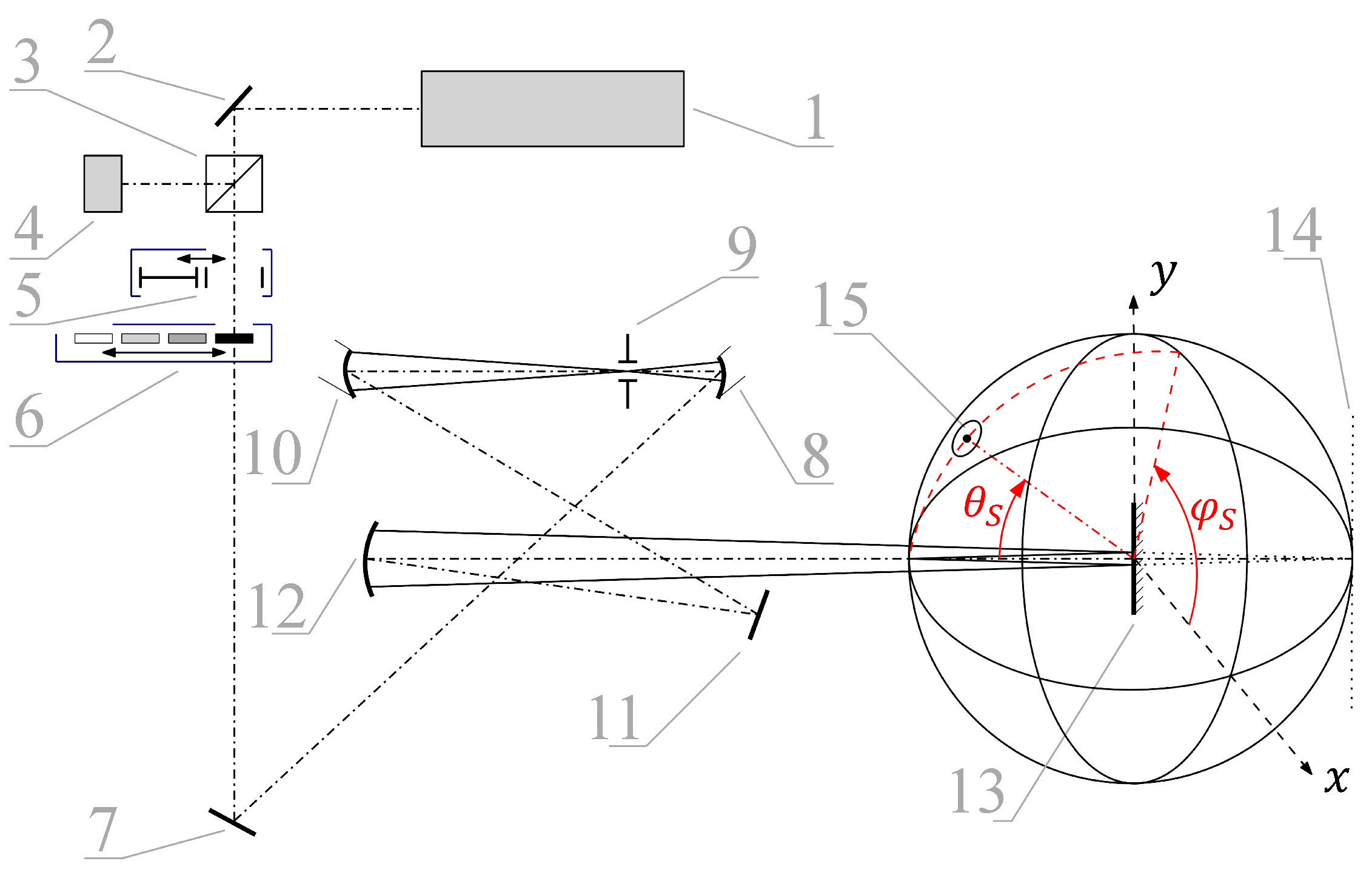
Angle-resolved scattering (ARS) measurements were performed using the goniometric type of 3D scatterometer developed and constructed at the Institute of Physical Engineering, Brno University of Technology (see
Figure 1). Multiple wavelengths (457.9 nm, 514.5 nm, and 647.1 nm) were selected for this measurement using a horizontally polarised argon ion laser Innova 70C (Coherent, Inc., Santa Clara, CA, USA) light source. By using the second channel (implemented to compensate for the potential instability of the laser light source during the measurements), we achieved higher stability and reliability for the instrument, measured data, and the results obtained. The optical system based on the reflective optical elements enables us to smoothly change the selected wavelength without any adjustments to the optical system. A spatially filtered laser light was focused on the back surface of the detecting sphere around the sample with a radius of 160 mm. The size of the approximately circular spot illuminating the sample was up to 4 mm in diameter. The goniometric movement of the detector (positions expressed by angles
and
) with a solid angle of acceptance
sr enabled us to measure the scattered light from the sample to the reflective half-space in the detecting hemisphere using a temperature-compensated APD410A2 UV enhanced Si avalanche photodetector (Thorlabs, GmbH., Bergkirchen, Germany). The samples were positioned perpendicularly to the incident laser light (angle of incidence:
). In order to achieve a higher dynamic range for the measured data, the intensity of the incident laser light beam was attenuated by a set of neutral density filters, which also protects the detector in the case of dangerous levels of illumination. In order to ensure valid data, a calibration diffuse reflectance optical standard Spectralon SRS-99-010 (Labsphere, Inc., North Sutton, NH, USA) was measured for selected wavelengths.
The measurements were performed for polar angles,
, with an interval of 3–60° and for four azimuthal angles 45°, 135°, 225°, and 315° chosen so that the detector moves in a plane tilted with respect to the plane of polarization by 45°. For a given value of the polar angle
, the experimental ARS data were represented by an average of the values measured for these four azimuthal angles. This approach was chosen because the SDT cannot take into account the polarization of light, and the described mean value is the same as that measured for a completely nonpolarized incident light. The ARS data for all four samples are shown in
Figure 2. All measurements were performed according to the procedure recommended in [
34].
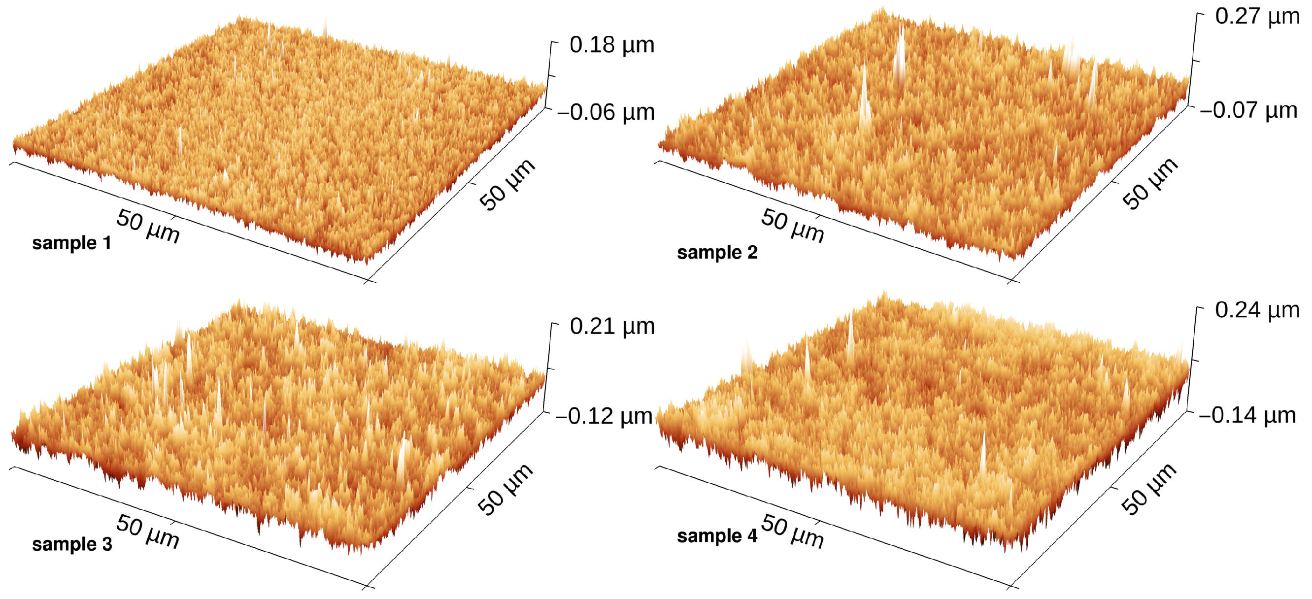
A Dimension Icon microscope (Bruker Corporation, Billerica, MA, USA) was used to obtain AFM scans of the topography of the rough samples. The measurements were performed using RTESPA-525 probes (Bruker Corporation, Billerica, MA, USA) in the tapping mode on an area of 50 × 50
m. The measurements in this relatively large area were necessary because of the need to characterize the part of the roughness with low spatial frequencies. The topography of the samples measured by AFM is shown in
Figure 3. The AFM scans were processed using the Gwyddion software (version 2.59) to obtain the PSDF as a function of the spatial frequencies.
5. Data Processing
The measured ARS data were processed using the least squares method, with the data measured for all three wavelengths (647.1 nm, 514.5 nm, and 457.9 nm) processed simultaneously. The PSDF is determined on the basis of its parametrization using a model that provides a sufficient number of parameters (degrees of freedom) to describe its course with sufficient accuracy. The least-squares method is then used to find the values of the parameters corresponding to the best fit of the experimental data.
The model using an exponential of a quadratic spline was chosen for the PSDF. This means that, on the individual sub-intervals, this is given as
where the index
distinguishes individual sub-intervals, with the border points given by the nodes at the positions
. For convenience, it is also useful to consider nodes at the origin and infinity as
and
. A schematic representation of this model is depicted in
Figure 4. The symbols
,
, and
denote the coefficients in the quadratic polynomials, which must be chosen such that the PSDF and its first derivative are continuous. It should be noted that this type of function was chosen because it is suitable for modeling a PSDF exhibiting rapid decrease with growing spatial frequency. How this model is used and what parameters are sought in the processing of the experimental data depends on whether
,
, or
is used; therefore, this will be discussed individually for each case.
The correspondence between the PSDF values for the given spatial frequency and the ARS measured at normal incidence for the given wavelength and the polar angle can be understood through the relation
, which is valid for
and
(see (
7)). In the case of
, this correspondence is not exact because the correction term
(
11) exhibits more complicated dependence. Since the range of measured wavelengths and polar angles is limited, the range of spatial frequencies, where the PSDF can be determined from the scattering experiment, is limited by
where the subscripts min and max denote the minimum and maximum values. This interval of spatial frequencies corresponds to region II depicted in
Figure 4.
In the case of the approach using
, the calculated values depend only on the PSDF evaluated for the spatial frequencies between
and
, which means that only the model describing the PSDF inside region II is required. Two nodes of the quadratic spline were chosen at the limiting points
and
, and four additional nodes at positions 0.001, 0.002, 0.004, and 0.008 nm
lying between these limiting values are introduced in order to describe the PSDF with sufficient accuracy. The resulting model has
node points and
sub-intervals covering the region from
to
. This corresponds to the model depicted in
Figure 4 if regions I and III are disregarded. The coefficients in the quadratic polynomials on these sub-intervals must be chosen such that the PSDF and its derivative are continuous at
points joining these sub-intervals, which results in a model requiring
parameters. The linear terms in the quadratic splines, which are related to the PSDF derivatives at the node points, as
,
can be used to specify
n of these degrees of freedom. The remaining degree of freedom is related to the absolute value of the PSDF, and it is convenient to specify it by means of the quantity
which express the contribution to the rms value of the heights of roughness
from spatial frequencies in region II.
In the approach using , it is also not necessary to consider what the PSDF looks like outside of region II, and the same parametrization as for can be used to specify the PSDF. However, the formula for contains a factor depending on the total rms value of the heights , which is an additional parameter of this model. In principle, the value of should always be greater than the value of . However, to investigate how well the factor in depending on describes the ARS data, we decided not to enforce this condition and consider it to be independent of the PSDF values.
The approach using
is more complicated because knowledge of the PSDF for all spatial frequencies is required, although it should be noted that values outside of region II result in a relatively small correction (see (
11)) to the values expressed using the
. The parametrization inside region II is performed in the same way as for the previous two approaches. In order to define the PSDF in regions I and III, we tried to devise the simplest model possible. Only one segment of the quadratic spline is used in region I. The continuity conditions at the point joining regions I and II and the condition that any reasonable PSDF should have a zero derivative at origin
fully specify the coefficients in the quadratic polynomial for this segment. This means that no additional parameters are needed to define the PSDF in region I. The approach used to deal with region III is based on the assumption that for large values of wavevector, the PSDF behaves as a Gaussian function, i.e., it is proportional to
for some value of
. In order to ensure that this Gaussian function transitions correctly to the part defined in region II, it is necessary to introduce an additional node,
, and define the segment between
and
such that the PSDF and its derivative are continuous at these points. The position of this node was chosen as
nm
. Because these continuity conditions fully specify the quadratic polynomial for this spline segment, only one additional parameter,
, is introduced in the resulting model. This model corresponds to the situation depicted in
Figure 4. The total rms value of the heights
then corresponds to the value calculated as a sum of contributions from all three intervals: I, II, and III, and it is given as
It is evident that the role of is to control the size of , i.e., how much the PSDF in the interval above contributes to and that the inequality is always satisfied.
The overview of the approaches used to evaluate the ARS data and the parameters sought within the processing by the least-squares method is presented in
Table 2.
The measurement procedure did not provide any obvious method on how to assign weights to individual experimental points, and since the ARS data cover the dynamic range of more than two magnitudes, it was not possible to assume that all of them contribute with the same weight. The problem of a large dynamic range was solved by representing the measured ARS data by their logarithm
, and equal (unit) weights were then assumed for these points. The merit function was defined as
where the superscripts “exp” and “th” distinguish the experimentally and theoretically determined quantities. The summation is performed over the experimental points, i.e., over the measured wavelengths and measured polar scattering angles. The quality of the fits achieved using individual models for the calculation of ARS can be compared by means of the regression standard error, defined as
where
is the residual sum of squares,
N is the number of experimental points, and
P is the number of sought parameters.
The reflectance in the formulae for ARS was calculated using optical constants determined for the single-wafer silicon with a smooth surface, which was the same type as that used to prepare the rough samples. A thin, native-oxide layer represented by a thin homogeneous layer with optical constants corresponding to amorphous SiO was assumed to be on top of the silicon surface; however, this has a negligible effect on the calculated values of normal reflectance, .
6. Results
6.1. Results Obtained by Processing the ARS Data
The values of the parameters determined by processing the measured ARS data are shown in
Table 3.
The determined PSDFs are then shown in
Figure 5. The fits to the theoretical curves corresponding to
are shown in
Figure 2.
The values of the regression standard error
, together with the values of this quantity relative to the value
achieved using
, are also shown in
Table 3. The best agreement with the experimental data was achieved using
, followed by
, which gave worse fits, and
, which resulted in the worst fits. This order of the qualities of the fits was the same for all four samples. The differences in the quality of the fits are minimal in the case of sample 1 (with the smallest roughness) and grew with increasing roughness height. For the rougher samples (3 and 4), the
and especially
lead to much worse agreement between the experimental data and theoretical predictions than the exact approach,
.
In the approaches and , it is also possible to determine the total rms value of the heights of roughness . Unfortunately, the values determined using the approximate approach, , are incorrect, with the exception of sample 1 with the smallest roughness. The value determined for samples 2, 3, and 4 is smaller than the value , which is physically impossible. The reason why these smaller values were determined is that was sought as a parameter independent of . It is possible to apply the least-squares method with the restriction that cannot be smaller than . The value of is then increased so that it matches the value of , but the quality of the fits is slightly worse.
It should be emphasized that if the scattering experiment was performed only for one wavelength of light, then it would not be possible to determine the total rms value of the heights in
and
. In [
5], where only one wavelength was used, and the model corresponding to
was used to evaluate the experimental data, it was necessary to fix the total rms value of the heights in the value determined from measurements of coherent reflectance.
The method of combining the ARS data measured for several wavelengths proved to be quite challenging. It was found that the errors in the absolute values of the measured ARS data in the order of a few percent significantly affected the determined value of and also decreased the quality of the fits. For this reason, it was important to ensure that the laser serving as a light source provides stable output power and that the scatterometer is properly calibrated using the Spectralon reference. The need to reduce the errors caused by the shifts in the absolute values was one reason why a second channel monitoring the output level of the laser was introduced in the experimental setup.
6.2. Comparison with the Results Obtained by AFM
The values of
and
obtained by using AFM are also shown in
Table 3. These values were calculated by numerically evaluating the integrals in (
15) and (
14) for the PSDF obtained by processing the AFM scans.
When comparing the heights of roughness determined by ARS and AFM, it is useful to look at the quantity , which represents the contribution from region II, i.e., the region of spatial frequencies covered by the measured ARS data. A reasonable agreement with deviations lower than 2 nm was obtained for the three approaches , , and . The approach gave the best agreement, with a value of determined by AFM for the rougher samples 3 and 4. This is surprising because it resulted in the poorest quality in terms of the fits. In our opinion, this does not mean that it works better than the other approaches; instead, we should look for another explanation for why the values determined from ARS are slightly higher than those corresponding to AFM.
The values obtained by agree reasonably well with those obtained by AFM, with the deviations following the same trends as in the case of .
Although the scatterometer allows for measurements for larger polar scattering angles, the ARS data considered in this work were limited to 60°. The reason is that the formula derived using the SDT is not able to correctly describe scattering for large values of
, as was shown in [
5].
6.3. Comparison of the Multi-Wavelength Approach and Point-by-Point Method Applied for Individual Wavelengths
The method that uses the ARS data evaluated in a point-by-point fashion to recover the PSDF is often used. This contrasts with the method used in this work, where the PSDF is given using a suitable model, and the ARS data are processed using the least-squares method. The point-by-point method cannot be used in the multi-wavelength approaches, in which the total rms value of the heights is sought in addition to the values of the PSDF. Moreover, the use of the parametrized PSDF model is unavoidable in the exact approach
because the ability to evaluate the PSDF for any spatial frequency is required to determine the correlation function needed in the evaluation of the integral (
11).
However, in the approach
, there is no dependency on the total rms value of the heights
, and it is possible to consider the ARS data separately for each wavelength and apply the corresponding formula (see (
7)) to recover the PSDF in a point-by-point fashion. The region of spatial frequencies where the PSDF can be recovered is different for each wavelength. In order to perform a sensible comparison of the results obtained for individual wavelengths, we can calculate the rms value of the heights from a sub-interval of spatial frequencies common to all three wavelengths. This contribution, which will be denoted as
, is calculated as
where
Note that while the interval
is an intersection of intervals where the PSDF can be determined using the ARS data for specific wavelengths, the interval
used to calculate
in (
14) represents their union. In order to clarify the meaning of the various rms values of the heights used to present the results, a short overview is presented in
Table 4. The values of
determined for each wavelength are shown in
Table 5, together with the value obtained by processing the data for all three wavelengths simultaneously by the least-squares method and
approach. The determined values increase with increasing wavelength, which is exactly the behavior that the dependency on the total rms value of the heights introduced in
and
should compensate for.
6.4. Discussion and Summary
It is possible that this discrepancy between the roughness parameters obtained by ARS and AFM is caused by the non-uniformity of the roughness on the sample. ARS was measured using the light spot, illuminating relatively large parts of the samples; therefore, it should provide good information about the mean roughness. However, the AFM scans were performed on much smaller parts of the sample, and the non-uniformity in roughness could make the determined roughness parameters dependent on the choice of the point on the sample selected for the AFM scan. In order to check for the presence of the non-uniformity, five additional AFM scans were measured for different parts of the selected sample (sample 2). It was found the rms values of the heights determined from these scans showed mutual differences of up to 0.7 nm.
Another possible reason leading to this discrepancy is related to the process of anodic oxidation used to prepare rough surfaces. It is possible that, in the case of very rough surfaces, where the anodic oxidation is applied for the longest period, it results not only in roughening the surface but also in the change in its structure, which then leads to the change in its optical properties (reflectance). This would then influence the roughness parameters determined by the optical method.
However, another reason might be related to the structures resembling spikes, which are visible in the AFM scans in
Figure 3. The description of these spikes as a part of the random roughness of the surfaces, which are assumed to be generated by the Gaussian process, is most likely incorrect. Therefore, it is possible that these structures contribute to the scattered light differently than was assumed in the derived formulae.
The application of the exact approach, , on multi-wavelength data was successful in determining both the PSDF and the total rms value of the heights of the investigated samples. Although the approximate approaches and are appealing because they are much easier to implement than the exact approach, the presented results showed that they failed to produce satisfactory results when used to process multi-wavelength data. The approach may be useful for a point-by-point method if only single-wavelength data are available. However, depending on the roughness of the samples, there may be other theoretical approaches that are more suitable for the application of the point-by-point method.
7. Conclusions
Angle-resolved scattering was measured for four samples of randomly rough silicon surfaces. The samples were selected so that each exhibited a different level of roughness, with the rms values of the heights ranging from approximately 12 nm for the smoothest sample to approximately 24 nm for the roughest samples. The measurements were performed for a normal incidence of light and three wavelengths of 457.9 nm, 514.5 nm, and 647.1 nm. The scatterometer developed and constructed at the Institute of Physical Engineering, Brno University of Technology, was used for the measurements.
The formulae derived using the scalar diffraction theory and the assumption of roughness generated by the Gaussian process were used to interpret the experimental data. The exact result derived using the SDT contains a rather complicated integral involving the correlation function, and knowledge of the PSDF for all spatial frequencies is required to evaluate the resulting ARS. However, if certain approximations are made, it is possible to recover a familiar correspondence between the ARS measured for a given scattering angle , wavelength , and the PSDF function evaluated at the spatial frequency . Two such approximations are considered. The ARS data for all three wavelengths were processed simultaneously, and the PSDF was determined within the relevant region of spatial frequencies. It was found that the exact approach and both its approximations gave reasonable agreement with results obtained using AFM.
The ARS values calculated using the exact approach and one of its approximations also exhibit a certain dependence on the total rms value of the heights of roughness. By simultaneously processing the data for all three wavelengths, it was possible to seek the value of this parameter in addition to the values of the PSDF. It should be emphasized that this parameter characterizes the roughness with all spatial frequencies, whereas the values of the PSDF are determined only in a limited interval of spatial frequencies. The total rms values of the heights determined using the exact approach are in reasonable agreement with the results obtained by AFM. Unfortunately, the approximate approach, which results in a much simpler formula, resulted in incorrect values of this quantity.
Although we consider it to be the main result, it should be noted that the possibility of recovering the total rms value of the heights of roughness is not the only reason why it is advantageous to combine ARS data for several wavelengths. The multi-wavelength method allows us to verify the validity of the theoretical approach. This is achieved by checking that the same roughness parameters give correct predictions for the ARS measured at different wavelengths. If only one wavelength is used, then it is difficult to verify whether the used approach works well for the investigated samples, and if an incorrect approach is used, then this most likely results in errors in the determined roughness parameters.
It was found that the accuracy of the ARS measurements is crucial for the successful application of the multi-wavelength method. Therefore, we would like to improve our experimental setup to improve its accuracy in our future work. Increasing the number of measured wavelengths and extending the covered spectral region, especially to the ultraviolet region, would also be highly desirable. The theoretical approach used did not allow us to consider the influence of the polarization of light, and, moreover, it was not possible to apply it at large scattering angles. This represents another area that we would like to address in our future work.


 ,
, 


