Abstract
Raman spectroscopy, measured by a Raman spectrometer, is usually disturbed by the instrument response function and noise, which leads to certain measurement error and further affects the accuracy of substance identification. In this paper, we propose a spectral reconstruction method which combines the existing maximum a posteriori (MAP) method and deep learning (DL) to recover the degraded Raman spectrum. The proposed method first employs the MAP method to reconstruct the measured Raman spectra, so as to obtain preliminary estimated Raman spectra. Then, a convolutional neural network (CNN) is trained by using the preliminary estimated Raman spectra and the real Raman spectra to learn the mapping from the preliminary estimated Raman spectra to the real Raman spectra, so as to achieve a better spectral reconstruction effect than merely using the MAP method or a CNN. To prove the effectiveness of the proposed spectral reconstruction method, we employed the proposed method and some traditional spectral reconstruction methods to reconstruct the simulated and measured Raman spectra, respectively. The experimental results show that compared with traditional methods, the estimated Raman spectra reconstructed by the proposed method are closer to the real Raman spectra.
1. Introduction
A spectrometer is a basic optical detection instrument that can obtain the spectral information of the measured object. At present, various spectrometers have been widely used in color measurement, gas composition analysis, agricultural medicine, food safety and other fields [1,2,3,4,5,6], and have become among the most important optical detection instruments. Among them, the Raman spectrometer [7,8,9], which is composed of a probe and a spectrometer, is a rapidly developed instrument in recent years. The Raman spectrometer can qualitatively analyze and identify various molecular structures and material types with few samples. In the past decade, the Raman spectrometer has been widely used in biology and analytical chemistry research because of its non-destructive, fast and real-time detection characteristics, and has achieved many significant research results. However, as an indispensable component of the Raman spectrometer, the non-ideality of the spectrometer usually makes it unable to present the real spectrum well. Specifically, due to the influence of the instrument response function, also known as the bandwidth function, the measured Raman spectra commonly contain spectral distortion, which leads to certain measurement error and further affects the accuracy of substance identification combining with noise. In order to overcome the shortcoming, an efficient method is to utilize spectral reconstruction methods to process the measured Raman spectra.
Spectral reconstruction, also known as spectral deconvolution [10,11,12,13,14,15,16,17,18,19,20,21,22,23,24,25,26,27,28,29,30,31,32,33], is among the most important issues in the field of spectral instrument signal processing. The purpose of spectral reconstruction is to obtain the estimated spectra closer to the real spectra from the degraded spectra with prior knowledge such as the instrument response function. Researchers have developed a variety of spectral deconvolution methods, with two main types—spatial domain-based spectral deconvolution [13,14,15,16,17,18,19,20,22,23,24,25,26,27,28,29,30,31,32,33,34] and frequency domain-based spectral deconvolution [10,11,12]. Among them, spatial domain-based spectral deconvolution can directly perform more intuitive and understandable operations on the measured spectra in the spatial domain. With the increase in spectral sampling points, early spatial domain-based spectral deconvolution methods usually cause ill-posed problems [21]. Therefore, regularization is necessarily introduced to enforce stability as well as incorporate prior knowledge about the solution. For instance, the authors of [22] upgraded the original Richard–Lucy (RL) method [17], and the improved spectral deconvolution method adopts a stopping condition curve, which is used to control the method to stop iteration before overfitting. Jin et al. [23] proposed a spectral reconstruction method which combines the Levenberg–Marquardt (LM) algorithm [24,25] with a well-known LED spectral model [26] to recover the degraded LED spectra. The specific process of this method is to use the LED spectral model to fit the measured spectra to eliminate high-frequency measurement errors such as noise, and then the LM algorithm is used to deconvolute the preprocessed spectra. The authors of [27] upgrade this method by directly introducing the regularization term, which enables the upgraded method to reconstruct most spectra, rather than be limited to LED spectral reconstruction. A spectral reconstruction method based on the maximum a posteriori (MAP) estimation framework was proposed in [28]. This method uses the Huber–Markov function as the regularization term, which can suppress the noise and retain the high-frequency spectrum, simultaneously. In addition to these methods, there are many spectral reconstruction methods with regularization [29,30,31,32,33], which can effectively solve most of the spectral reconstruction problems.
Nevertheless, Raman spectra often contain many narrowband spectra. Due to the larger spectral distortion, traditional spectral deconvolution methods are often difficult to use to recover the narrowband spectra very accurately. Therefore, compared with general spectral reconstruction, Raman spectral reconstruction is more challenging. At present, many researchers have proposed methods for Raman spectral reconstruction [34,35,36,37]. Angelini et al. [34] proposed a method based on peak identification through FMFs to identify Raman spectra automatically. A denoising method [35] for Raman spectra with a low SNR based on feature extraction was proposed by Zhao et al. Based on the Hilbert Vibration Decomposition (HVD) method, Raman spectra were decomposed into two components. The peaks were located in the first component and compensated by those in the second component. Finally, Gaussian signals are used to reconstruct Raman peaks from strong noise and the baseline. Barton et al. [36] demonstrated how Savitzky–Golay (S–G) smoothing may be enhanced with maximum likelihood estimation in order to prevent significant deviation from the true Raman signal yet retain the robust smoothing properties of the S-G filter. As an emerging technology, deep learning (DL) can employ the collected datasets to train a deep neural network, so as to directly build the restoration model from input data to output data without complex mathematical operations. DL is a branch of machine learning (ML). DL is an algorithm based on an artificial neural network to learn the characteristics of data. Unlike ML, which requires artificial feature extraction, DL has no complex artificial feature extraction process, and the feature extraction process can be completed automatically through a deep neural network (DNN). DL often requires a large number of training datasets to achieve better results. Common deep learning frameworks include TensorFlow, caffe2, Keras, PyTorch, and DyNet. At present, DL has been widely applied to the field of signal processing and classification [38,39,40,41,42,43,44,45], which provides a new possibility for designing spectral deconvolution methods that can effectively reconstruct Raman spectrum. In this paper, we propose a novel spectral reconstruction method which combines the MAP method [28] and deep learning (DL) to recover the degraded Raman spectrum. The proposed method first employs the MAP method to reconstruct the measured Raman spectra, so as to obtain preliminary estimated Raman spectra. Then, a convolutional neural network (CNN) is trained by using the preliminary estimated Raman spectra and the real Raman spectra to learn the mapping from the preliminary estimated Raman spectra to the real Raman spectra. The main advantage of this method over the traditional methods is that it establishes the mapping from the preprocessed spectra to the real spectra, so as to achieve a better spectral reconstruction effect than merely using the traditional methods or a CNN.
The structure of this paper is as follows: Section 2 provides an overview of the background of spectral deconvolution, including the measured spectral model and the spectral deconvolution model. Next, the proposed method is discussed in Section 3. In Section 4, we compare the effect of the proposed method and some traditional spectral reconstruction methods to reconstruct the simulated and measured Raman spectra to prove its effectiveness. The conclusion is presented in Section 5.
2. Basic Concepts
2.1. The Measured Spectral Model
In spectral instruments, the degraded spectrum can generally be expressed as the convolution of the original spectrum and the instrument response function, as well as the noise superimposed on the spectrum, which is mainly produced during the measurement process. Therefore, the process can usually be modeled as
where is the real spectrum, is the instrument response function, is measurement noise, and is the measured spectrum. Since the pixels of CCD used for sampling are discrete, the mathematical model of the measured spectrum can be written as
where j represents the number of sampling points in the measured spectrum. The instrument response function of the spectrometer is the effect of the combination of the response functions of its multiple optical elements. Researchers used to characterize the instrument response function of the spectrometer through a variety of functions, among which the Gaussian function is the closest and most widely used compared to the real instrument response function. For simplification, in this paper, the Gaussian function is selected to estimate the response function of the spectrometer instrument, as shown below:
where and indicate the wavelength corresponding to the peak point and the standard deviation of the function. In practical applications, Equation (3) is usually used to fit the measured spectrum of the Hg–Ar lamp or laser light source, so as to obtain the instrument response function of the spectrometer. Nevertheless, the instrument response functions corresponding to different wavelengths of the spectrometer are different, that is, the two parameters and of each instrument response function are different. In view of this, the mathematical model for the measured spectrum can be updated as the form of matrix.
where is the instrument response function matrix including the instrument response functions of all wavelengths of the spectrometer, and its expression is
where j is the number of sampling point of the spectrometer. Thus, , and in Equation (4) can be redefined as , and .
Researches show that the noise [46] of the spectrometer can be classified into four main parts: readout noise, dark noise, fixed pattern noise, and photoelectron noise. Although the reasons for these kinds of noise are different, they are all Gaussian white noise. Considering that these types of noise are independent of each other, the overall noise can be regarded as the superposition of each kind of noise, which is also Gaussian white noise.
2.2. Spectral Reconstruction Model
The purpose of spectral reconstruction is to obtain the estimated spectra closer to the real spectra from the degraded spectra with prior knowledge such as the instrument response function. Generally, spectral reconstruction can be converted into the minimization of the spectral reconstruction model. The spectral reconstruction model, also known as the objective function, can be obtained by the least-square principle, and can be written as
where represents the estimated spectra of real spectra, and .
Nevertheless, spectral deconvolution is ill-posed and extremely sensitive to the noise in the measured spectrum. Even very small noise may cause uncertainty in the solution of the estimated spectrum, resulting in a large amount of artificial noise generated in the estimated spectrum. To solve this, regularization is necessarily introduced to enforce stability as well as incorporate prior knowledge about the solution.
Therefore, a new spectral reconstruction model with a regularization term can be rewritten, and its expression is Equation (7).
where is a regularization term and α indicates the coefficient of regularization term. Researchers have proposed many regularization methods, such as Tikhonov regularization, Gaussian–Markov regularization, wavelet transforms regularization, and total variation regularization. Since so many types of regularization terms have different constraint functions, the appropriate regularization term is usually selected according to the specific reconstruction requirements. In addition, a non-negative constraint can be added to the estimated spectrum.
3. Raman Spectrum Reconstruction Method
3.1. Traditional Methods
As mentioned above, the estimation of the real spectrum can be obtained by selecting the appropriate regularization term to construct the objective function and solving it. The objective function can be solved by many traditional methods, among which, a MAP-based deconvolution method has great advantages in dealing with the broadening effect of narrowband spectrum [28]. The method uses the Huber–Markov regularization term, which can suppress the noise and restore the high-frequency spectrum (narrowband spectrum) by reasonably selecting µ, simultaneously.
The algorithm uses Euler–Lagrange equation and the Neumann boundary condition to minimize objective function with respect to R, and the expression is shown in Equation (9):
The expression of and in Equation (9) can be easily obtained by calculation, as shown in Equations (10) and (11), respectively.
Therefore, the estimated spectrum can be obtained by using a successive iteration, as shown in Equation (12).
where tj is the time step parameter used for controlling the convergence rate.
3.2. Proposed Method
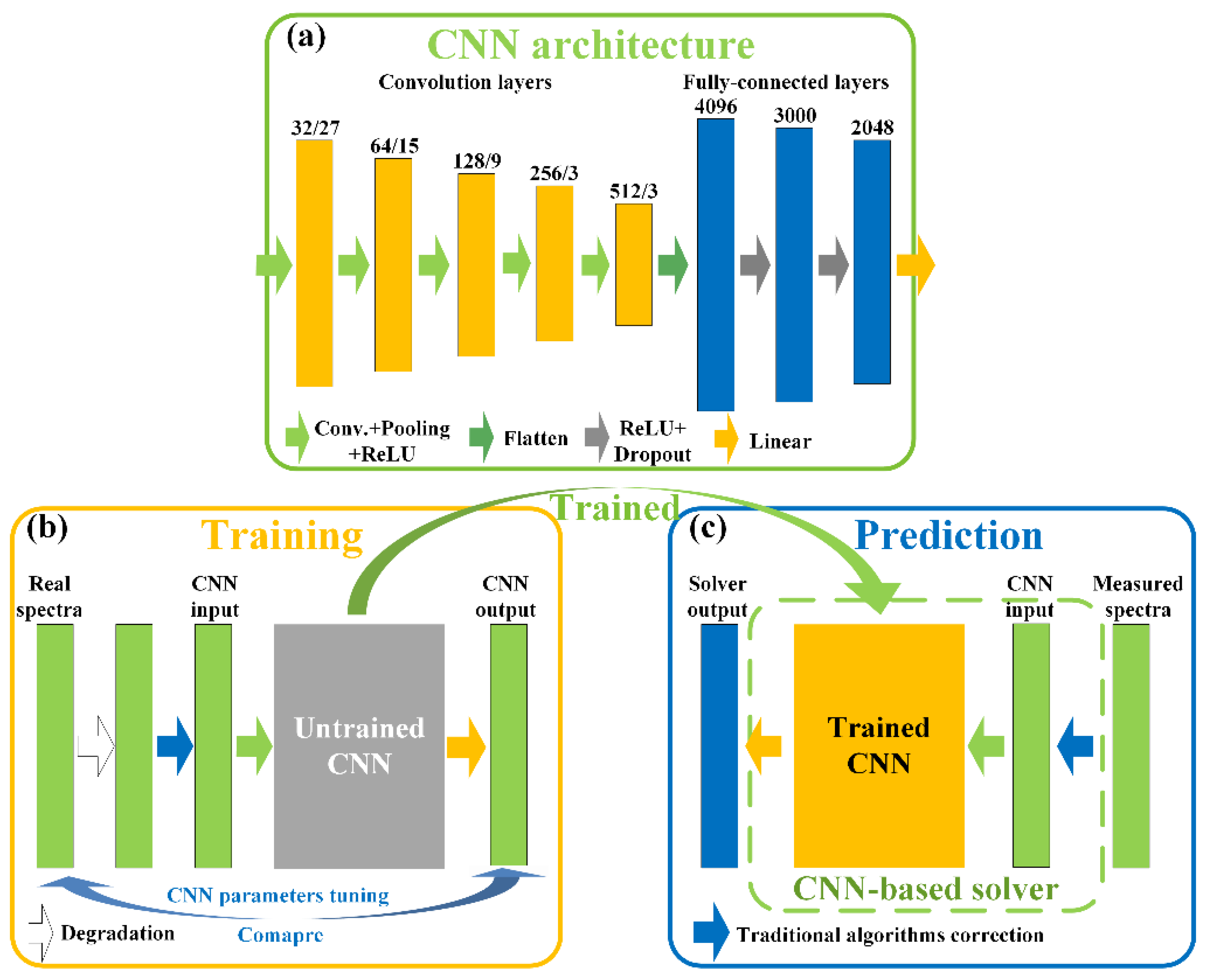
Due to the employ of traditional deconvolution methods, the reconstructed Raman spectrum has been much improved compared with the measured Raman spectrum. However, the reconstruction effect of these methods on the measured Raman spectrum is still unsatisfactory, the peak value of reconstructed narrowband spectra is often lower than the real spectra. To overcome these limitations of traditional methods, a novel spectral reconstruction method which combines the MAP method and a CNN framework to enhance the spectral reconstruction effect of degraded Raman spectrum is proposed. The proposed method first employs the MAP method to reconstruct the measured Raman spectra, so as to obtain preliminary estimated Raman spectra. Then, a CNN is trained by using the preliminary estimated Raman spectra dataset and the real Raman spectra dataset to learn the mapping from the preliminary estimated Raman spectra to the real Raman spectra. The main advantage of this method over the traditional methods is that it establishes the mapping from the preprocessed spectra to the real spectra, so as to achieve a better spectral reconstruction effect than merely using the traditional methods or a CNN. Figure 1 illustrates the schematic of the proposed method. There are three parts of this system: CNN architecture, training and predicting.

Figure 1.
Schematic of the proposed method. (a) CNN architecture. (b) CNN training stage. (c) Trained CNN predicting process.
The CNN architecture consists of eight learnable layers, including five convolution layers and three fully connected layers. Convolution layers are employed for feature extraction in non-linear mapping between the preliminary estimated Raman spectra and real Raman spectra. The fully connected layers are employed for synthesizing the features extracted by the convolution layers, so as to reconstruct the real Raman spectrum. Moreover, Figure 1a shows the detailed information of learnable kernels. After each convolution layer, the ReLU and max pooling which is used for down-sample are employed. Then, the output data of convolution layers are flattened and used as the input data of fully connected layers. ReLU and dropout operations are performed on the first two fully connected layers, while the third fully connected layer is followed by a linear activation function, which will directly return the data of the third fully connected layer.
In the CNN training stage, first of all, it is necessary to establish a real Raman spectra dataset, which can be downloaded from the website or constructed using multiple Lorentz functions. Then, the measured Raman spectra dataset can be simulated from the real Raman spectrum dataset combined with the instrument response function and noise. Next, the measured Raman spectra dataset is preprocessed by the traditional method such as the MAP method, and the preliminary estimated Raman spectra is used as the input dataset of CNN. Details of the construction of these datasets will be described in next section. Finally, Raman spectra in the output dataset are compared with the corresponding spectra in the real Raman spectra dataset to adjust the structural parameters of a CNN to minimize the loss function, so as to obtain the trained CNN. There are many kinds of loss functions, in this paper, the mean square error is selected:
where is the i-th term of the real spectrum R, is the i-th term of the reconstruction spectrum , and represents the square of L2 norm.
In the CNN prediction stage, the measured Raman spectrum needs to be deconvoluted by the MAP method first, and then the preliminary estimated Raman spectrum is used as the input of the CNN to obtain final estimated Raman spectrum. It should be noted that in addition to the MAP method, other traditional methods can also be employed to deconvolute the measured Raman spectrum, but the traditional method selected in the CNN predicting process should be consistent with the method in the training stage. Compared with traditional methods, the main advantage of the proposed method is that it builds the mapping from the preliminary estimated Raman spectra to the real Raman spectra, rather than just deconvolution of the measured Raman spectra, so that the preliminary reconstruction results are more similar to the real Raman spectra. Compared with directly using a CNN to establish mapping relationship, the reconstruction method in this paper first employs the MAP method to extract more spectral features, which improves the quality of CNN input data, thus enhancing the ability of the CNN to obtain better estimates.
4. Simulations and Experiments
To prove the effectiveness of the proposed spectral reconstruction method, we employed the proposed method and some classical traditional spectral reconstruction methods to reconstruct the simulated and measured Raman spectra, respectively.
4.1. CNN Training Stage
Two synthetic Raman spectra datasets were established, both of which contain approximately 2000 Raman spectra. The real spectra of the first synthetic dataset were established by the combination of multiple Lorentz functions. We randomly generate multiple Lorentz functions within the spectral measurement range, and their peaks, central wavenumbers and full width at half maximum (FWHM) were also randomly determined within a certain range. More details of the first synthetic Raman spectrum dataset are shown in Table 1.

Table 1.
Details of the first synthetic Raman spectrum dataset.
The real spectra of the second synthetic dataset were obtained by denoising and smoothing Raman spectra in the KnowItAll Raman spectral dataset [47]. The real spectra as the CNN output datasets. Then, the measured Raman spectra dataset was generated by employing the real spectra combined with the measured spectrum model (Equation (2)). Finally, the traditional method (MAP method) was employed to deconvolute the measured spectra, and the preliminary estimated Raman spectra are used as the input datasets of a CNN.
The number of training, validation, and test spectra were randomly assigned in the ratio of 5:1:1 for both of the real Raman spectra datasets and CNN input datasets, respectively. The validation spectra were used to estimate the number of epochs and adjust the hyperparameters. The Adam optimizer with the batch size of 32 implemented in TensorFlow 2.0 (Google, Mountain View, CA, USA) was employed, and all calculations were performed on NVIDIA GeForce RTX 3070Ti (NVDIA, Santa Clara, CA, USA) graphics processing unit (GPU). The whole training stage took about 30 min. After a CNN is trained, the time for reconstructing the input spectrum is very short, but considering that it takes approximately 10 s for the MAP method to reconstruct the Raman spectrum, the process of reconstructing the spectrum with the proposed method lasts approximately 10 s.
4.2. Simulations
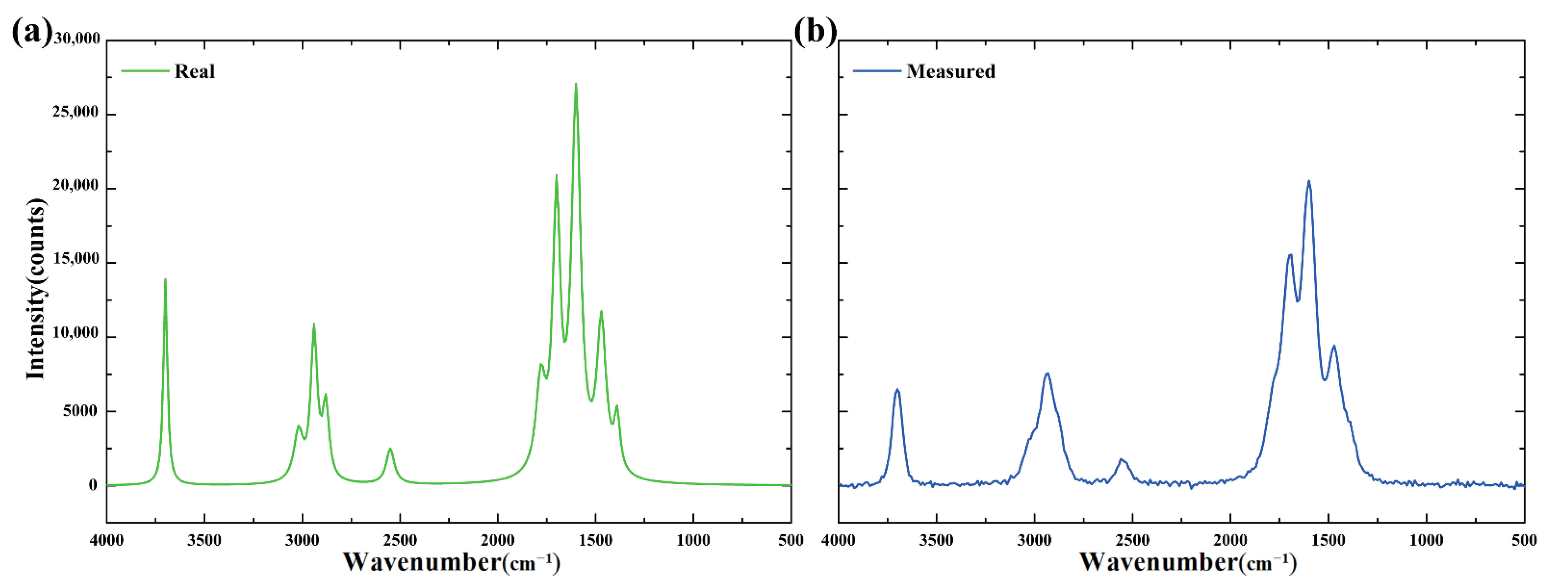
According to the instrumental characteristics of a self-developed Raman spectrometer, a measured Raman spectrum was simulated by combining a real Raman spectrum which was developed based on multiple Lorentz functions and the instrument response functions. For simplicity, the instrument response functions corresponding to all wavelengths are set to the same value, and the spectral range of the Raman spectrum is between 200 and 4000 cm−1. The simulated measurement was obtained by convolving the real Raman spectrum with the instrument response function and adding noise. The real Raman spectrum and the measured Raman spectrum are shown in Figure 2a,b, respectively.
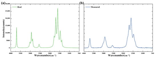
Figure 2.
Simulated real and measured Raman spectrum. (a) Real Raman spectrum. (b) Measured Raman spectrum.
As shown in Figure 2, owing to the effect of the instrument response function, the narrow band parts of the measured Raman spectrum are degraded, causing the decline of spectral resolution, and even the degradation of three spectral peaks into one peak and five spectral peaks into three peaks. This leads to a certain measurement error, and further affects the accuracy of substance identification in combination with noise.
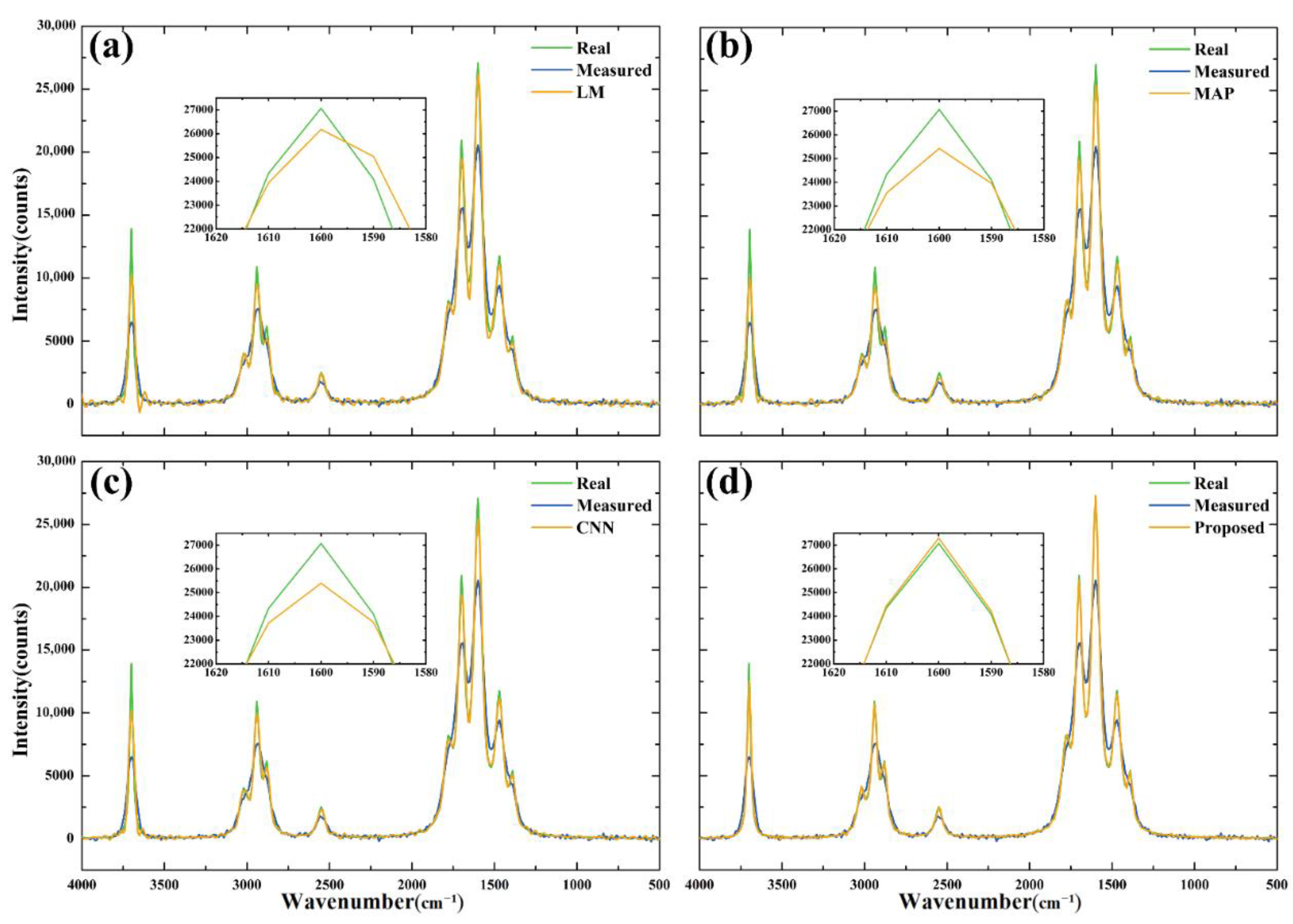
Then, the measured Raman spectrum was reconstructed by the LM method [27], the MAP method [28] and proposed method. In addition, to show the superiority of the proposed spectral reconstruction method over using a CNN directly, a CNN is also trained with measured Raman spectra dataset and real Raman spectra dataset to estimate the real Raman spectrum. The estimated spectra of the four methods are shown in Figure 3a–d.
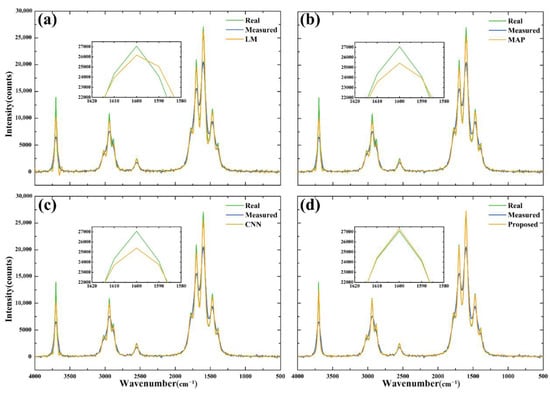
Figure 3.
Reconstruction results of the Raman spectrum by several methods. (a) the LM method; (b) the MAP method; (c) the CNN method; (d) the proposed method.
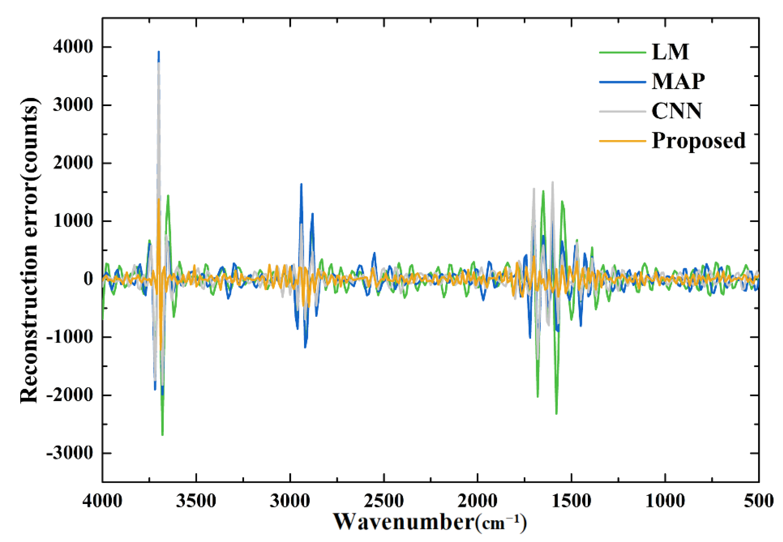
Figure 3a–d show that these methods have a certain correction effect on the measured Raman spectrum. Compared with the measured spectrum, the estimated spectra of all the four methods are more similar with the real spectrum. The effect of the two traditional methods is similar, a CNN method is slightly weaker, while the proposed method is undoubtedly the best of the four methods. The main reason for this phenomenon is due to the proposed method is a deconvolution model based on the MAP method, which is equivalent to reconstructing the estimated spectrum of the MAP method towards the real spectrum again. To further analyze the reconstruction effect of the four methods on the Raman spectrum, the real Raman spectrum is subtracted from their reconstructed spectra, respectively, and the reconstruction errors are obtained, as shown in Figure 4.
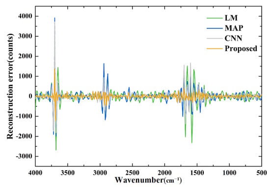
Figure 4.
Reconstruction error of the Raman spectrum by several methods.
It can be seen from the figure that the reconstruction error of the proposed method is significantly lower than that of the other three methods, especially near the peak points of the Raman spectrum. Moreover, root mean square errors (RMSEs) and normalized mean square errors (NMSEs) of the reconstruction results of these methods are calculated to quantify the reconstruction effect of each method. These two parameters can be calculated by Equations (14) and (15).
where is the i-th term of the real spectrum R, and is the i-th term of the reconstruction spectrum .
Table 2 shows the calculation results of these two parameters. The results show that the two parameters calculated from the reconstruction results obtained by the proposed method are much smaller than those obtained by other methods, which is consistent with the results in Figure 3.
Table 2.
RMSEs and NMSEs of the reconstruction results of four methods.
4.3. Influence of Noise
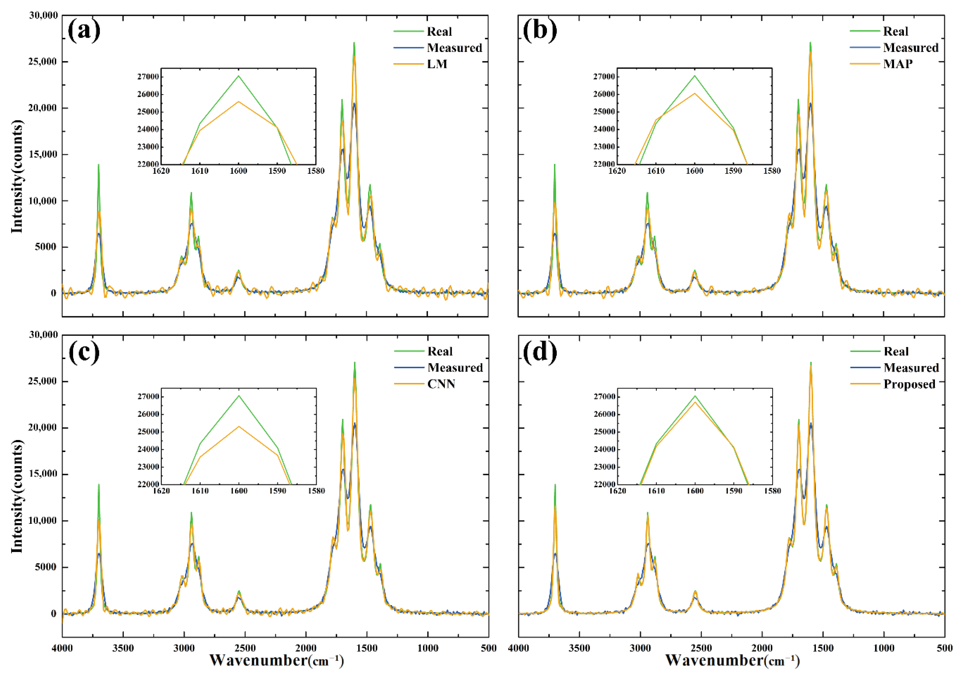
The measured Raman spectrum is always accompanied by noise. Although noise has been added to the simulated spectrum in Section 4.2, the influence of the intensity of noise on the proposed reconstruction method is not considered. After generating the measured Raman spectrum without noise, add the noise of levels 10, 50, 100 and 200 in turn to obtain four measured Raman spectra with the same degree of spectral degradation but different noise levels. Next, the four methods were employed to obtain estimated spectra. The four simulated Raman spectrum are shown in Figure 5, and the estimated spectra of the measured spectrum (noise level = 200) obtained by the four methods are shown in Figure 6, the reconstruction errors of the four methods are shown in Figure 7.
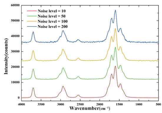
Figure 5.
Four simulated spectra with different noise levels.
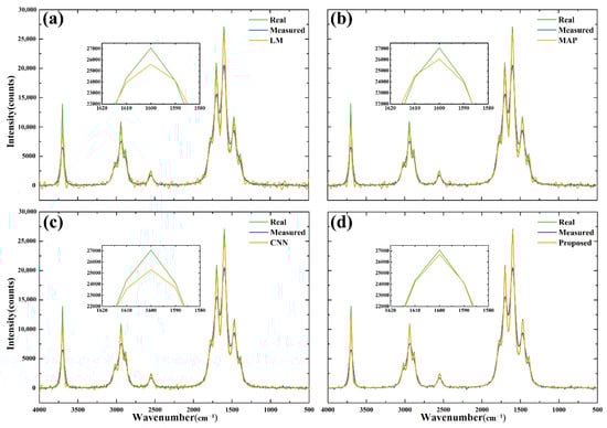
Figure 6.
Estimated spectra obtained by the four methods. (a) the LM method; (b) the MAP method; (c) the CNN method; (d) the proposed method.
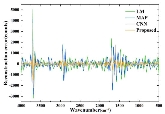
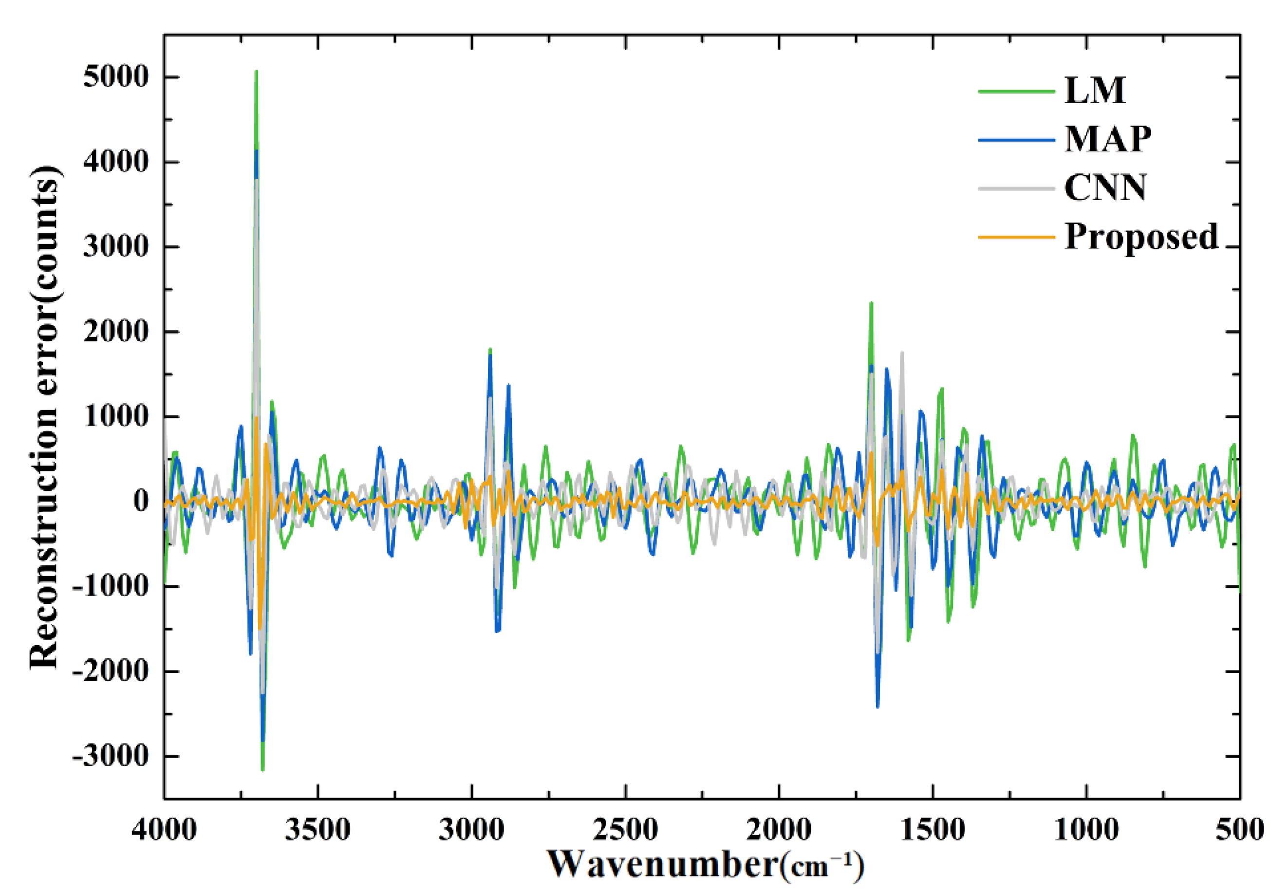
Figure 7.
Reconstruction errors of the Raman spectrum by several methods.
In Figure 6, the proposed method still shows an excellent reconstruction effect when the noise level is 200, as the reconstructed spectrum is essentially consistent with the real spectrum. Compared with the low noise situation, the estimated spectra obtained by the traditional methods have a greater degree of under correction, which is because these methods increase the regularization parameters to repress the noise. In addition, the estimated spectrum of the proposed method is smooth in the low-frequency regions, while other methods still have some residual noise. A similar conclusion can be drawn from Figure 7. In addition, comparing Figure 4 with Figure 7, we can find that the reconstruction error of the proposed method does not increase significantly when reconstructing the Raman spectrum with more noise, while the reconstruction error of the other three methods increases significantly. We also calculated the two parameters of the estimated spectra corresponding to the measured spectra, and the results are shown in Table 3. As can be seen from the table that with the increase in noise, both of the parameters of the estimated spectra obtained by the four methods increase. Even so, compared with other methods, the proposed method has more satisfactory results, which can simultaneously repress noise and reconstruct the narrowband spectrum effectively.
Table 3.
RMSEs and NMSEs of the reconstruction results of measured Raman spectra with different noises by four methods.
4.4. Experiments
Moreover, we carried out experiments to explore the effectiveness of this method on the real measured spectra, which were measured from several drug samples through a self-developed Raman spectrometer with a 785 nm laser source. All these measured Raman spectra were baseline corrected.
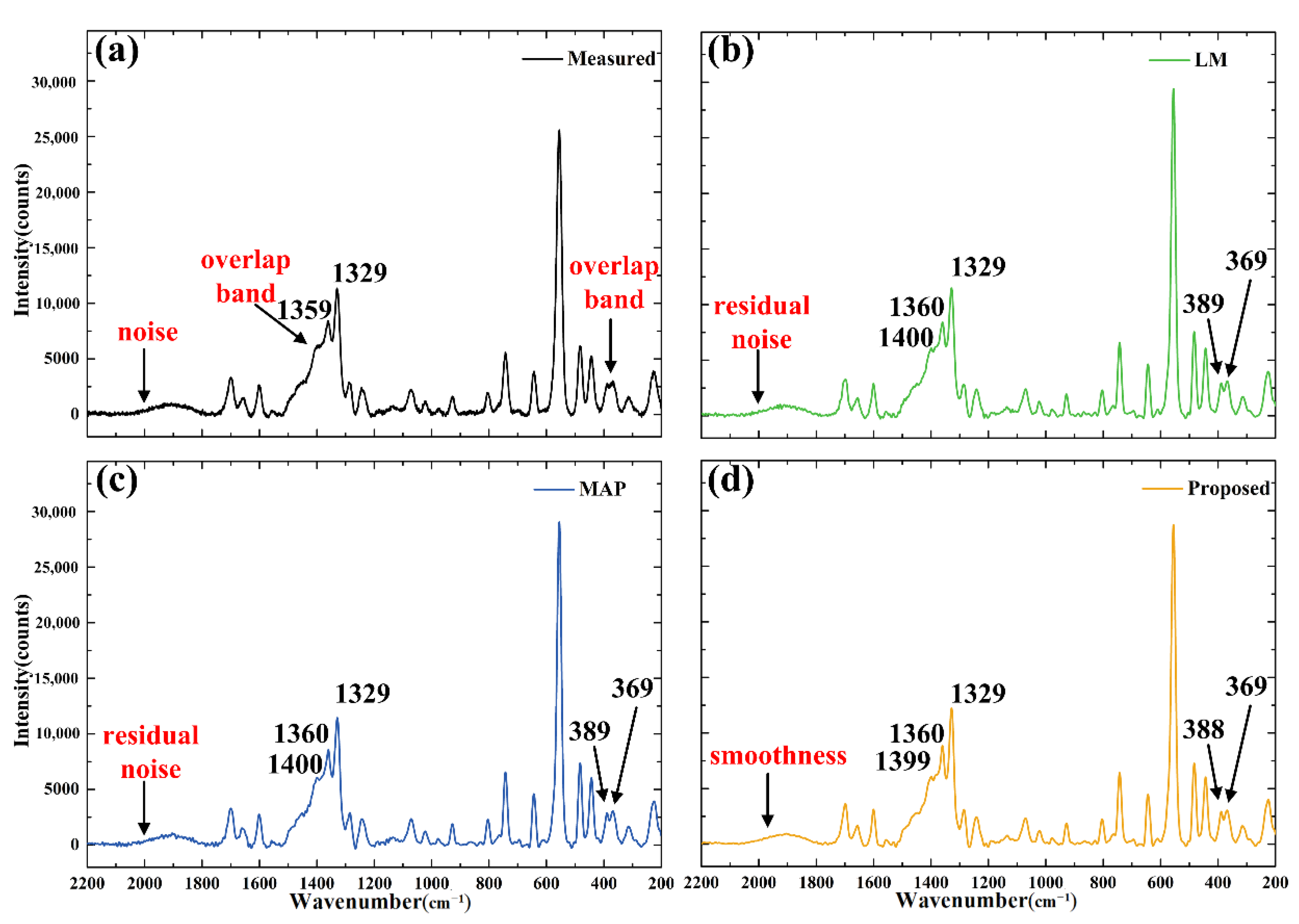
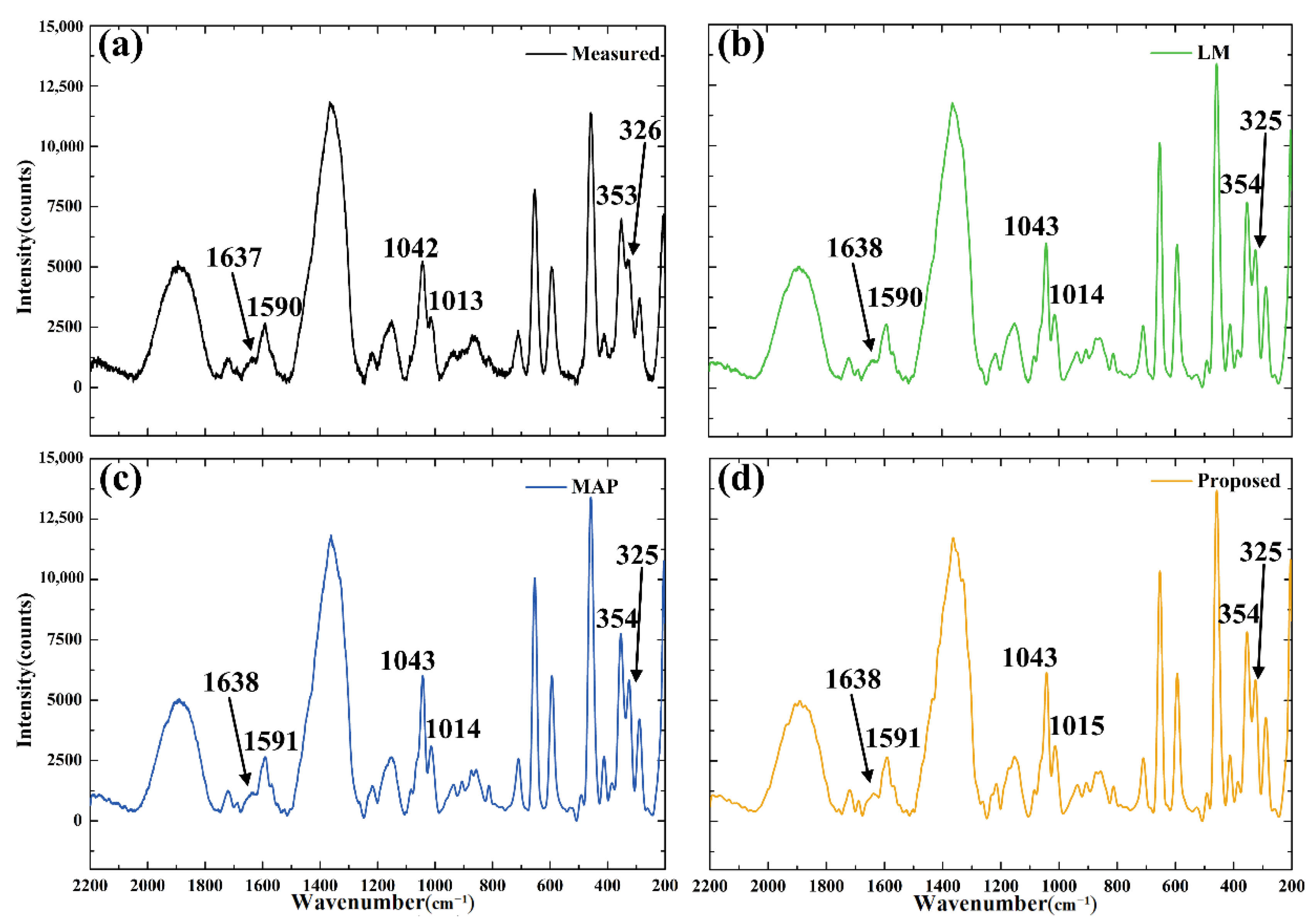
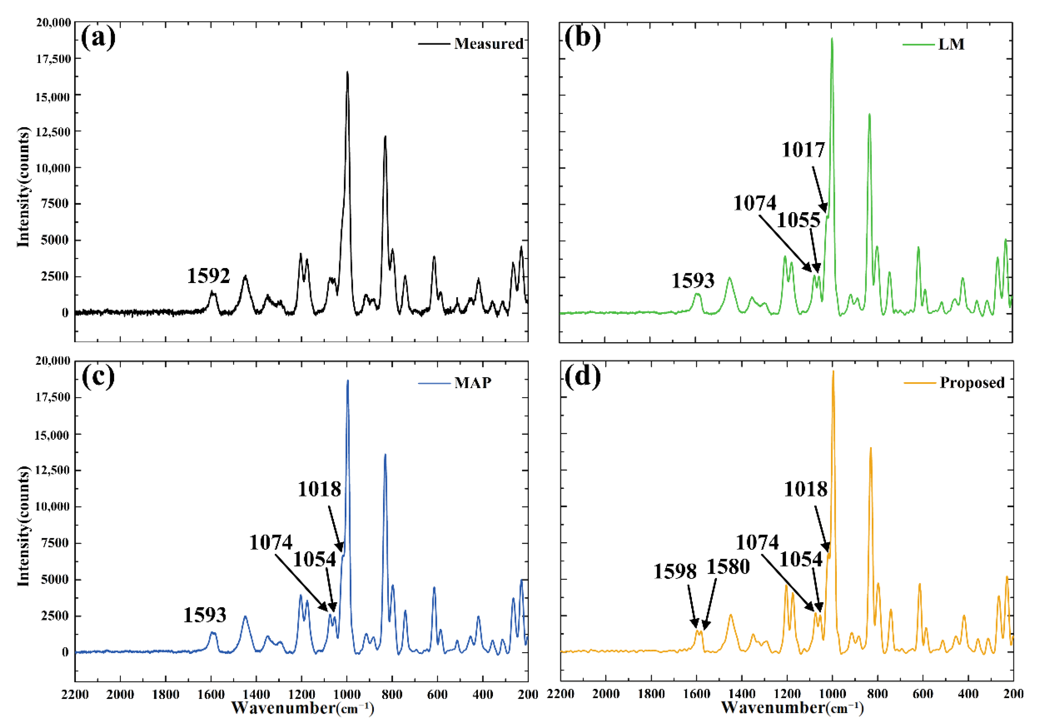
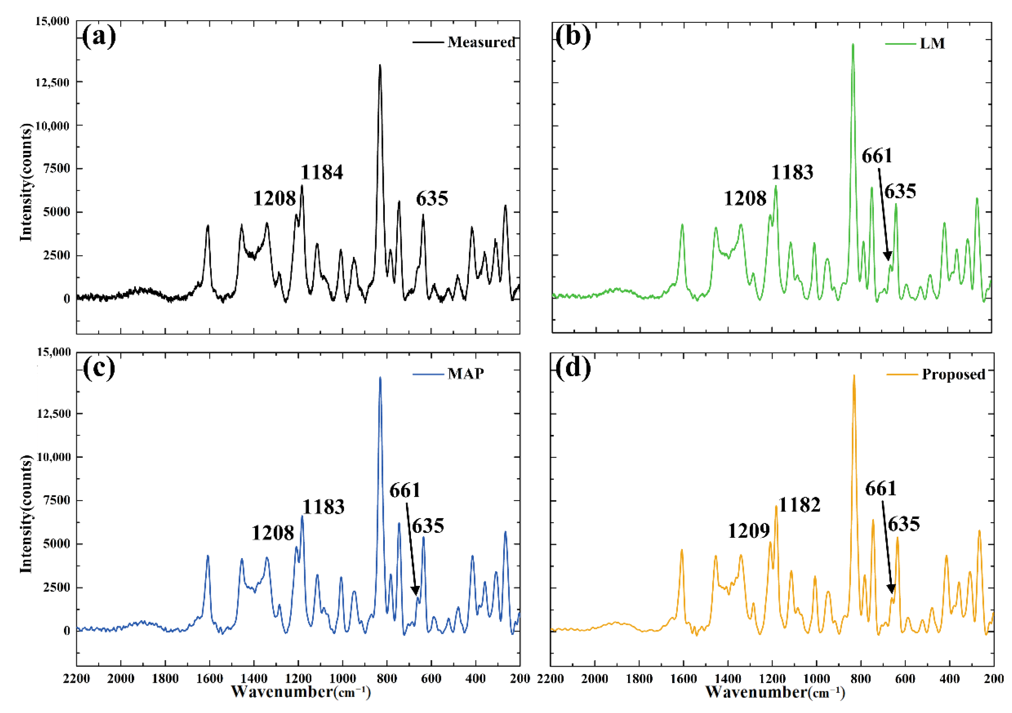
Figure 8a displays the measured spectrum of caffeine (C8H10N4O2) from 2200 to 200 cm−1. A linear spectrum corresponding to approximately 1400 cm−1 position of the Raman spectrometer was obtained by a tunable laser, and the instrument response function of the Raman spectrometer is obtained by Gaussian function fitting. Next, three methods were used to reconstruct the measured Raman spectrum of caffeine, respectively. The reconstruction results show that, the resolution of the estimated spectra obtained by the three methods has been improved, especially the overlap peak can be split into multiple peaks. However, the estimated spectra obtained by the two traditional methods can be observed obvious residual noise, while the reconstructed spectrum of proposed method is smooth in the flat region. In addition, Raman spectra of other three drug samples include ketamine (C13H16ClNO), methamphetamine (C10H15N) and ibuprofen (C13H18O2) were collected, and estimated spectra were obtained by three methods, and shown in Figure 9, Figure 10 and Figure 11, respectively. The estimated spectra of each sample obtained by three methods are similar to Figure 8. Therefore, from the perspective of spectrum reconstruction, the performance of the proposed method is the best of three tested methods.
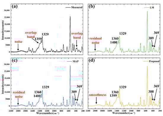
Figure 8.
(a) Caffeine (C8H10N4O2) measured spectrum and reconstructed spectra with spectral range from 2200 to 200 cm−1 by (b) the LM method; (c) the MAP method; (d) the proposed method.
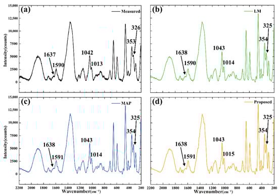
Figure 9.
(a) Ketamine (C13H16ClNO) measured spectrum and reconstructed spectra with spectral range from 2200 to 200 cm−1 by (b) the LM method; (c) the MAP method; (d) the proposed method.
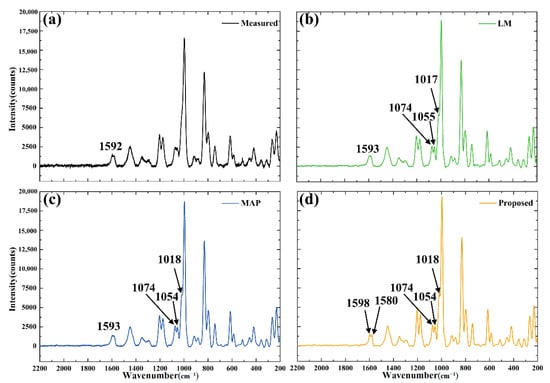
Figure 10.
(a) Methamphetamine (C10H15N) measured spectrum and reconstructed spectra with spectral range from 2200 to 200 cm−1 by (b) the LM method; (c) the MAP method; (d) the proposed method.
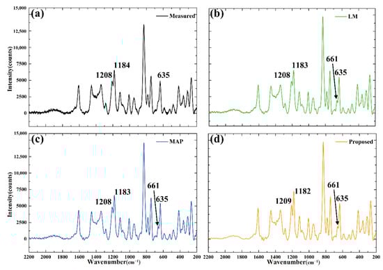
Figure 11.
(a) Ibuprofen (C13H18O2) measured spectrum and reconstructed spectra with spectral range from 2200 to 200 cm−1 by (b) the LM method; (c) the MAP method; (d) the proposed method.
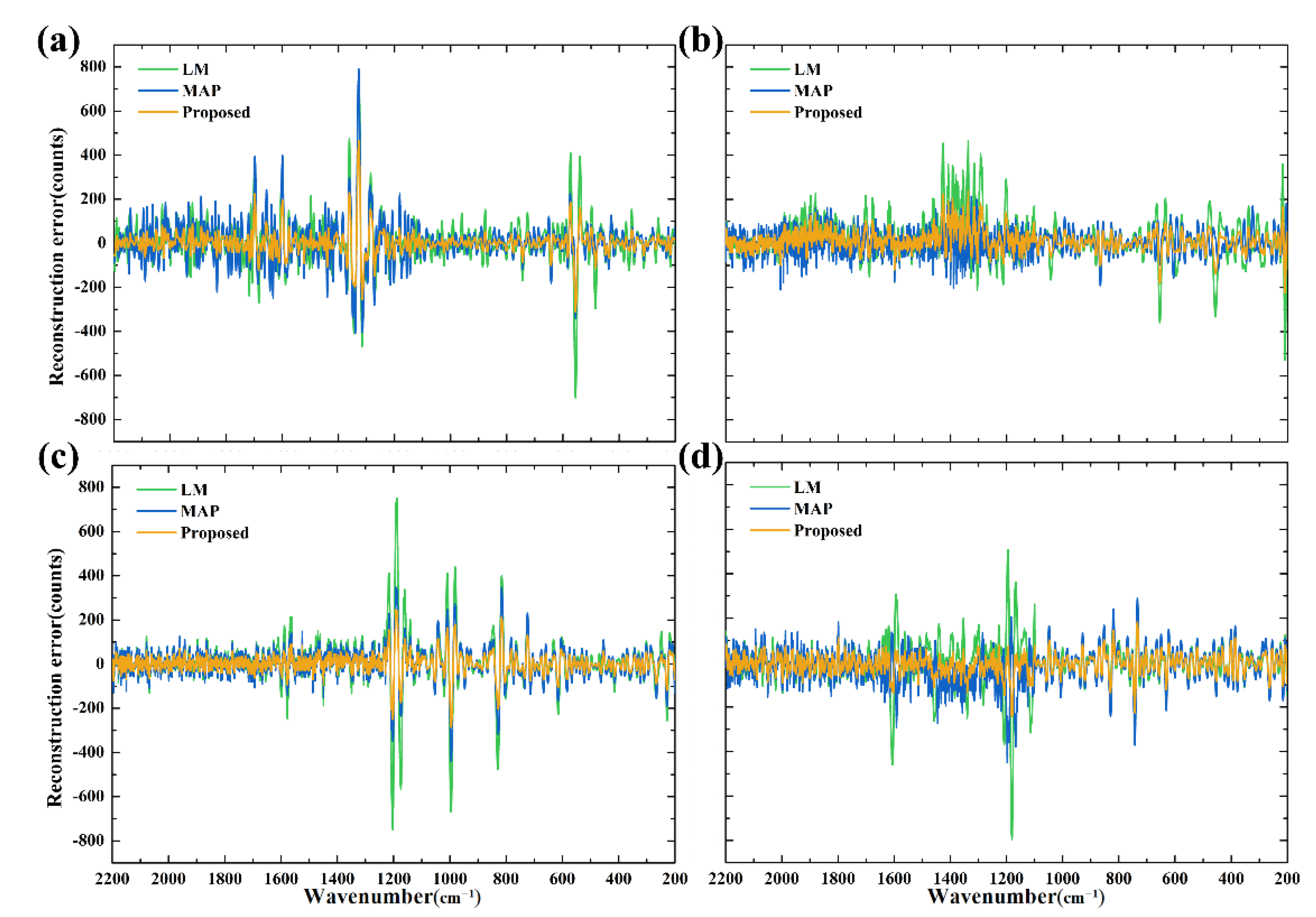
For these measured Raman spectra, the real spectra are unknown. In order to quantify the effects of various methods, the spectra in the sample dataset are selected as the reference spectra. The reference Raman spectra are subtracted from their reconstructed spectra, respectively, and the reconstruction errors are obtained, as shown in Figure 12.

Figure 12.
Reconstruction errors of Raman spectra by several methods. (a) Caffeine; (b) ketamine; (c) methamphetamine; (d) ibuprofen.
From the reconstruction errors of Raman spectra by each method, it can be seen that although the reconstruction effect of the three methods is superior, the estimated spectra obtained by the proposed method are the closest to the reference spectra in the sample dataset, and the reconstruction errors are significantly smaller than the other two methods. Similarly, taking the reference spectra as the standard spectra, we calculated the RMSEs and NMSEs of the reconstruction results of these methods, and the results are shown in Table 4. Moreover, the parameter correlation coefficient (CC) is also employed to quantify the reconstruction performance of these methods, which is defined as
where is the i-th term of the reconstruction spectrum , represents the i-th term of the corresponding spectral data in the sample dataset, is the average of , and is the average of . The calculation results of the parameter CC are shown in Table 5.
Table 4.
RMSEs and NMSEs of the reconstruction results of different measured Raman spectra by four methods.
Table 5.
The results of the CC of each method.
Table 4 shows that the RMSE and the NMSE calculated from the reconstruction results obtained by the proposed method are much smaller than those obtained by other methods, which is consistent with the results in Figure 12. The results in Table 5 show that, the parameter CC of the three methods is improved. Even so, compared with other methods, the proposed method has more satisfactory results, the value of the CC is closest to 1. All the experimental results prove the superiority of the proposed method.
5. Conclusions
The Raman spectrometer is a rapidly developed instrument in recent years. The Raman spectrometer can qualitatively analyze and identify various molecular structures and material types with few samples. However, as a component of the Raman spectrometer, the non-ideality of the spectrometer usually makes it unable to present the real spectrum well. Due to the influence of the instrument response function, the measured Raman spectra commonly contain spectral distortion, which leads to certain measurement error and further affects the accuracy of substance identification combining with noise. In this paper, we propose a novel spectral reconstruction method which combines the MAP method and the DL to recover the degraded Raman spectrum. First, the MAP method is employed to reconstruct the measured Raman spectra, so as to obtain preliminary estimated Raman spectra. Then, a CNN is trained by using the preliminary estimated Raman spectra and the real Raman spectra to learn the mapping from the preliminary estimated Raman spectra to the real Raman spectra. The main advantage of this method over the traditional methods is that it establishes the mapping from the preprocessed spectra to the real spectra, so as to achieve a better spectral reconstruction effect than merely using the traditional methods or a CNN. To prove the effectiveness of the proposed spectral reconstruction method, we employed the proposed method and some traditional spectral reconstruction methods to reconstruct the simulated and measured Raman spectra, respectively. The RMSE, the NMSE and the CC were used to quantify the reconstruction effect. The experimental results show that compared with traditional methods, the estimated Raman spectra reconstructed by the proposed method are closer to the real Raman spectra.
Author Contributions
Data curation, Z.Z.; Funding acquisition, Q.Z.; Software, Z.Z. and L.H.; Writing—original draft, Q.Z.; Writing—review & editing, Q.Z. and L.H. All authors have read and agreed to the published version of the manuscript.
Funding
This research was funded by the National Key R&D Program of China, Grant No. 2017YFE0301205.
Institutional Review Board Statement
Not applicable.
Informed Consent Statement
Not applicable.
Data Availability Statement
The authors confirm that the data supporting the findings of this study are available within the article.
Conflicts of Interest
The authors declare no conflict of interest.
References
- Yang, Z.; Albrow-Owen, T.; Cai, W.; Hasan, T. Miniaturization of optical spectrometers. Science 2021, 371, eabe0722. [Google Scholar] [CrossRef] [PubMed]
- Wang, H.; Nan, L.; Huang, H.; Yang, P.; Song, H.; Han, J.; Wu, Y.; Yan, T.; Yuan, Z.; Chen, Y. Adaptive measurement method for miniature spectrometers used in cold environments. Appl. Opt. 2017, 56, 8029–8039. [Google Scholar] [CrossRef] [PubMed]
- Bandeliuk, O.; Assaf, A.; Bittel, M.; Durand, M.; Thouand, G. Development and Automation of a Bacterial Biosensor to the Targeting of the Pollutants Toxic Effects by Portable Raman Spectrometer. Sensors 2022, 22, 4352. [Google Scholar] [CrossRef] [PubMed]
- Jadidi, A.; Mi, Y.; Sikström, F.; Nilsen, M.; Ancona, A. Beam Offset Detection in Laser Stake Welding of Tee Joints Using Machine Learning and Spectrometer Measurements. Sensors 2022, 22, 3881. [Google Scholar] [CrossRef] [PubMed]
- Merrick, T.; Bennartz, R.; Jorge, M.; Pua, S.; Rausch, J. Evaluation of Plant Stress Monitoring Capabilities Using a Portable Spectrometer and Blue-Red Grow Light. Sensors 2022, 22, 3441. [Google Scholar] [CrossRef]
- Otto, C.; Grauw, C.; Duindam, J.; Sijtsema, N.; Greve, J. Applications of Micro-Raman Imaging in Biomedical Research. J. Raman Spectrosc. 2017, 28, 143–150. [Google Scholar] [CrossRef]
- Hidi, I.; Grjasnow, A.; John, H.; Weber, K.; Popp, J.; Hauswald, W. Noise Sources and Requirements for Confocal Raman Spectrometers in Biosensor Applications. Sensors 2021, 21, 5067. [Google Scholar] [CrossRef]
- Yang, D.; Liu, Q.; Guo, J.; Wu, L.; Kong, A. Cavity Enhanced Multi-Channels Gases Raman Spectrometer. Sensors 2021, 21, 3803. [Google Scholar] [CrossRef]
- Innocenti, S.; Balbas, D.; Pezzati, L.; Fontana, R.; Striova, J. Portable Sequentially Shifted Excitation Raman Spectroscopy to Examine Historic Powders Enclosed in Glass Vials. Sensors 2022, 22, 3560. [Google Scholar] [CrossRef]
- Kauppinen, J.; Moffatt, D.; Cameron, D.; Mantsch, H. Noise in Fourier self-deconvolution. Appl. Opt. 1981, 20, 1866–1879. [Google Scholar] [CrossRef]
- Lórenz-Fonfría, V.; Villaverde, J.; Padrós, E. Fourier Deconvolution in Non-self-deconvolving Conditions. Effective Narrowing, Signal-to-Noise Degradation, and Curve Fitting. Appl. Spectroc. 2002, 56, 232–242. [Google Scholar] [CrossRef]
- Lórenz-Fonfría, V.; Padrós, E. The Role and Selection of the Filter Function in Fourier Self-Deconvolution Revisited. Appl. Spectroc. 2009, 63, 791–799. [Google Scholar] [CrossRef] [PubMed]
- Stearns, E.; Stearns, R. An example of a method for correcting radiance data for bandpass error. Color Res. Appl. 1988, 13, 257–259. [Google Scholar] [CrossRef]
- Woolliams, E.; Baribeau, R.; Bialek, A.; Cox, M. Spectrometer bandwidth correction for generalized bandpass functions. Metrologia 2011, 48, 164–172. [Google Scholar] [CrossRef]
- Yuan, J.; Hu, Z. High-order statistical blind deconvolution of spectroscopic data with a Gauss-Newton algorithm. Appl. Spectrosc. 2006, 60, 692–697. [Google Scholar] [CrossRef] [PubMed]
- Reiter, J. An algorithm for deconvolution by the maximum entropy method with astronomical applications. J. Comput. Phys. 1992, 103, 169–183. [Google Scholar] [CrossRef]
- Fish, D.; Brinicombe, A.; Walker, R. Blind deconvolution by means of the Richardson–Lucy algorithm. J. Opt. Soc. Am. A 1995, 12, 58–65. [Google Scholar] [CrossRef] [Green Version]
- Kennett, T.; Prestwich, W.; Robertson, A. Bayesian deconvolution I: Convergent properties. Nucl. Instrum. Methods 1978, 151, 285–292. [Google Scholar] [CrossRef]
- Kennett, T.; Prestwich, W.; Robertson, A. Bayesian deconvolution II: Noise properties. Nucl. Instrum. Methods 1978, 151, 293–301. [Google Scholar] [CrossRef]
- Kennett, T.; Prestwich, W.; Robertson, A. Bayesian deconvolution III: Applications and algorithm implementation. Nucl. Instrum. Methods 1978, 153, 125–135. [Google Scholar] [CrossRef]
- Hansen, P. Analysis of Discrete Ill-Posed Problems by Means of the L-Curve. SIAM Rev. 1992, 34, 561–580. [Google Scholar] [CrossRef]
- Eichstädt, S.; Schmähling, F.; Wübbeler, G.; Anhalt, K.L.; Bünger, L.; Krüger, U.; Elster, C. Comparison of the Richardson-Lucy method and a classical approach for spectrometer bandpass correction. Metrologia 2013, 50, 107–118. [Google Scholar] [CrossRef]
- Jin, S.; Huang, C.; Xia, G.; Hu, M.; Liu, Z. Bandwidth correction in the spectral measurement of light-emitting diodes. J. Opt. Soc. Am. A 2017, 34, 1476–1480. [Google Scholar] [CrossRef]
- Levenberg, K. A method for the solution of certain non-linear problems in least squares. Q. Appl. Math. 1944, 2, 164–168. [Google Scholar] [CrossRef] [Green Version]
- Marquardt, D. An Algorithm for Least-Squares Estimation of Nonlinear Parameters. J. Soc. Ind. Appl. Math. 1963, 11, 431–441. [Google Scholar] [CrossRef]
- He, G.; Zheng, L. A model for LED spectra at different drive currents. Chin. Opt. Lett. 2010, 8, 1090–1094. [Google Scholar] [CrossRef]
- Huang, C.; Chang, Y.; Han, L.; Chen, F.; Hong, J. Bandwidth correction of spectral measurement based on Levenberg–Marquardt algorithm with improved Tikhonov regularization. Appl. Opt. 2019, 58, 2166–2173. [Google Scholar] [CrossRef]
- Liu, H.; Zhang, T.; Yan, L.; Fang, H.; Chang, Y. A MAP-based algorithm for spectroscopic semi-blind deconvolution. Analyst 2012, 137, 3862–3873. [Google Scholar] [CrossRef]
- Liu, T.; Liu, H.; Chen, Z.; Lesgold, A. Fast Blind Instrument Function Estimation Method for Industrial Infrared Spectrometers. IEEE Trans. Ind. Inform. 2018, 14, 5268–5277. [Google Scholar] [CrossRef]
- Liu, H.; Li, Y.; Zhang, Z.; Liu, S.; Liu, T. Blind Poissonian reconstruction algorithm via curvelet regularization for an FTIR spectrometer. Opt. Express 2018, 26, 22837–22856. [Google Scholar] [CrossRef]
- Liu, T.; Liu, H.; Li, Y.; Zhang, Z.; Liu, S. Efficient Blind Signal Reconstruction with Wavelet Transforms Regularization for Educational Robot Infrared Vision Sensing. IEEE/ASME Trans. Mechatron. 2019, 24, 384–394. [Google Scholar] [CrossRef]
- Liu, H.; Zhang, Z.; Liu, S.; Liu, T.; Yan, L.; Zhang, T. Richardson–Lucy blind deconvolution of spectroscopic data with wavelet regularization. Appl. Opt. 2015, 54, 1770–1775. [Google Scholar] [CrossRef]
- Liu, H.; Liu, S.; Huang, T.; Zhang, Z.; Hu, Y.; Zhang, T. Infrared spectrum blind deconvolution algorithm via learned dictionaries and sparse representation. Appl. Opt. 2016, 55, 813–2818. [Google Scholar] [CrossRef]
- Angelini, F.; Santoro, S.; Colao, F. Chemical Identification from Raman Peak Classification Using Fuzzy Logic and Monte Carlo Simulation. Chemosensors 2022, 10, 295. [Google Scholar] [CrossRef]
- Zhao, X.; Liu, G.; Sui, Y.; Xu, M.; Tong, L. Denoising method for Raman spectra with low signal-to-noise ratio based on feature extraction. Spectrochim. Acta A 2021, 250, 119374. [Google Scholar] [CrossRef]
- Barton, S.; Ward, T.; Hennelly, B. Algorithm for optimal denoising of Raman spectra. Anal. Methods UK 2018, 10, 3759–3769. [Google Scholar] [CrossRef]
- Machado, L.; Silva, M.; Campos, J.; Silva, D.; Cancado, L.; Neto, O. Deep-learning-based denoising approach to enhance Raman spectroscopy in mass-produced graphene. J. Raman Spectrosc. 2022, 53, 863–871. [Google Scholar] [CrossRef]
- Liu, H.; Fang, S.; Zhang, Z.; Li, D.; Li, K.; Wang, J. MFDNet: COllaborative poses perception and matrix Fisher distribution for head pose estimation. IEEE Trans. Multimed. 2021, 99, 2449–2460. [Google Scholar] [CrossRef]
- Li, Z.; Liu, H.; Zhang, Z.; Liu, T.; Xiong, N. Learning knowledge graph embedding with heterogeneous relation attention networks. IEEE Trans. Neural Netw. Learn. Syst. 2021, 33, 3961–3973. [Google Scholar] [CrossRef]
- Zhang, Z.; Li, Z.; Liu, H.; Xiong, N. Multi-scale dynamic convolutional network for knowledge graph embedding. IEEE Trans. Knowl. Data Eng. 2020, 34, 2335–2347. [Google Scholar] [CrossRef]
- Hansen, D. Using deep neural networks to reconstruct non-uniformly sampled NMR spectra. J. Biomol. NMR 2019, 73, 577–585. [Google Scholar] [CrossRef] [PubMed] [Green Version]
- Li, D.; Hansen, A.; Yuan, C.; Li, L.; Brüschweiler, R. DEEP picker is a deep neural network for accurate deconvolution of complex two-dimensional NMR spectra. Nat. Commun. 2021, 12, 5229. [Google Scholar] [CrossRef] [PubMed]
- Li, Y.; Xue, Y.; Tian, L. Deep speckle correlation: A deep learning approach toward scalable imaging through scattering media. Optica 2018, 5, 1181–1190. [Google Scholar] [CrossRef]
- Gu, Z.; Gao, Y.; Liu, X. Optronic convolutional neural networks of multi-layers with different functions executed in optics for image classification. Opt. Express 2021, 29, 5877–5889. [Google Scholar] [CrossRef] [PubMed]
- Chen, L.; Peng, B.; Gan, W.; Liu, Y. Plaintext attack on joint transform correlation encryption system by convolutional neural network. Opt. Express 2020, 28, 28154–28163. [Google Scholar] [CrossRef] [PubMed]
- Huang, C.; Xia, G.; Jin, S.; Hu, M.; Wu, S.; Xing, J. Denoising analysis of compact CCD-based spectrometer. Optik 2018, 157, 693–706. [Google Scholar] [CrossRef]
- The KnowItAll Raman Spectral Library. Available online: https://sciencesolutions.wiley.com/solutions/technique/raman/knowitall-raman-collection/ (accessed on 10 June 2022).

Publisher’s Note: MDPI stays neutral with regard to jurisdictional claims in published maps and institutional affiliations. |
© 2022 by the authors. Licensee MDPI, Basel, Switzerland. This article is an open access article distributed under the terms and conditions of the Creative Commons Attribution (CC BY) license (https://creativecommons.org/licenses/by/4.0/).