Article

Experimental Research on the Fluctuation Characteristics of Water Film Driven by Wind

1
Shenyang Key Laboratory of Aircraft Icing and Ice Protection, AVIC Aerodynamics Research Institute, Shenyang 110034, China
2
Liyang Aerodynamics Innovation Institute, Liyang 213300, China
3
College of Aerospace Engineering, Nanjing University of Aeronautics and Astronautics, Nanjing 210016, China
4
Key Laboratory of Icing and Anti/De-Icing, China Aerodynamics Research and Development Center, Mianyang 621000, China
*
Author to whom correspondence should be addressed.
Coatings 2022, 12(8), 1040; https://doi.org/10.3390/coatings12081040
Submission received: 28 May 2022 / Revised: 18 July 2022 / Accepted: 19 July 2022 / Published: 22 July 2022
(This article belongs to the Special Issue Superhydrophobic Surface for Anti-icing)

Abstract

:
A series of experimental studies were conducted to explore the fluctuation characteristics of the water film under the air flow condition with the research background of the anti-icing system. The dynamic measurement of the water film on the surface of the aluminum-based plate was achieved using the digital image projection measurement technology. The influence of diverse wind speeds and Reynolds numbers on the average water film thickness, fluctuation intensity, and velocity of the liquid film was analyzed. The piecewise characteristics of the wind speed and Reynolds number for the fluctuation characteristics of the water film were analyzed innovatively. The fluctuation characteristics and formation principle of each stage were also examined. The results had a significant impact on establishing and modifying the mesoscopic models of aircraft icing to improve the design methodology of the anti-icing process.

1. Introduction

Icing is a serious threat to aircraft flight safety as many aircraft accidents are caused by the icing phenomenon [1]. Icing is a phenomenon in which supercooled droplets from clouds impact on the leading edge of the airfoil and freeze [2]. Nowadays, most commercial aircraft use anti-icing or de-icing systems. The anti-icing system works by not letting the supercooled water droplets immediately freeze after the impact. In this way, a large number of supercooled water droplets are collected on the surface, hence forming a stable water film. In addition to the anti-icing system, many aircraft are coated with anti-icing coatings to solve the icing problem. Supercooled droplets on the anti-icing coating will converge to form a water film. The interaction between the water film and anti-icing coating can be obtained by studying the flow behavior of the water film on the surface. The water film on the surface begins to move gradually under the action of airflow shear [3,4]. During the flow process, the water film interacts with the aircraft surface and forms a gas–liquid interface with the air. The water film flow does not remain the same and may produce large fluctuations. Therefore, the study of the water film motion law can considerably improve the understanding of the solid–liquid interface. The anti-ice coating can be designed according to the flow characteristics of the water film.
For a better understanding and analysis of the mechanism of the water film flow, it is crucial to implement experimental methods to describe the phenomenon. Many scholars have conducted experimental studies on water film flow processes [5]. Rothmayer et al. [6] studied the water film flow process based on the boundary layer theory in fluid mechanics. Wang et al. [7] studied the flow process of the water film on a small size roughness surface based on the boundary layer theory at a high Reynolds number. Planquart et al. [8] developed the Level Detection and Record (LeDaR) technology at the Von Kaman Institute. Fluorescent dyes were added to the liquid, and the free surface of the liquid was characterized by the laser irradiation and charge-coupled device (CCD) imaging techniques. Similarly, Touron et al. [9] used the LeDaR technique to measure the horizontally layered two-phase flow in a rectangular cross-section pipe, and compared the spectral differences between the two-dimensional and three-dimensional wavy stratified flow patterns. Cherdantsev et al. [10] studied the process of the water film flow on the surface of a horizontal flat plate under the action of high-speed airflow shear and proposed the three-dimensional structure of the water film surface fluctuations and its possible mechanism. Zhang et al. [11] investigated the average thickness of the water film at different wind speeds based on the digital image projection (DIP) technique and studied the reflux phenomenon of the water film on the airfoil surface [12,13]. Chang et al. [14] used a planar laser-induced fluorescence method to analyze the thickness and fluctuation characteristics of the water film. However, the water film boundary extraction process used by Chang et al. required multiple splicing of the image to obtain the water film surface data. Therefore, it was difficult to perform a large-scale three-dimensional measurement. Leng et al. [15] investigated the water film thickness at a spot on the surface of a flat plate using a dispersive confocal displacement meter and proposed a new model to calculate the interfacial shear coefficient based on the results. However, there were some limitations when using this single-point measurement method to determine a large-scale liquid film flow. It can be observed that the current research on the water film is highly prevalent. However, research on the water film fluctuation characteristics of the airflow—water film interaction is still not very systematic.
The study of the water film flow on the surface plays a critical role in the design of an anti-icing system. Accurate measurement of the water film at large-scales has always been challenging in experiments. Therefore, this study aimed to develop a set of DIP technology to perform the global measurement of the large-scale liquid film flow on the flat, while the instantaneous visualization of the water film flow was achieved by the three-dimensional surface reconstruction of the water–air interface. This provided a lot of experimental data for the examination of the surface fluctuation characteristics of the liquid film on a large flat. The study of the water film flow in the anti-icing process has a certain guiding significance. In the subsequent sections, the experimental system and principles will be introduced, followed by the quantitative analysis of experimental results. Finally, the research conclusions will be summarized.

2. Experimental Setup

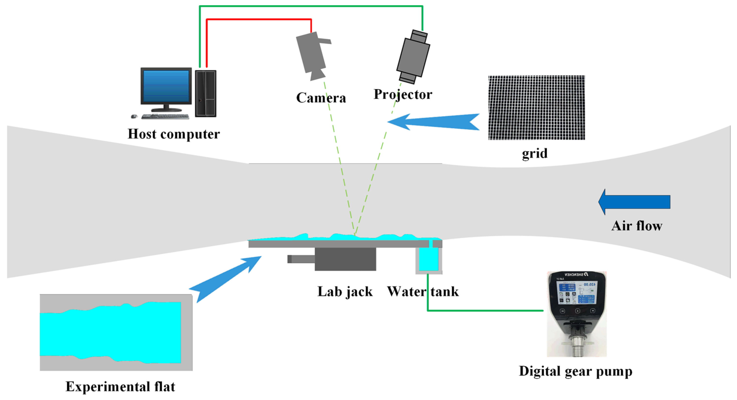
2.1. Construction of Measurement System

Figure 1 demonstrates the experimental system of the water film flow on the flat [16]. The air flowed into the experimental section of the wind tunnel after being rectified in the contraction section. Grilles and damping screens were installed upstream of the constriction section to ensure a uniform airflow. The cross-section area of the experimental section was kept as 300 mm × 75 mm. In order to facilitate the replacement of the experimental flat, a piece of removable glass was employed at the top of the experimental section. The experimental flat was an aluminum-based plate, and a lifting table was installed under it. In order to study the water film flow on the aircraft surface, the 2024/LY12 aluminum alloy was used. One end of the experimental flat was provided with a water outlet, which was connected with a water supply tank, while the water flow was regulated by a high-precision gear pump. At the same time, the CCD camera was used for the image acquisition with an acquisition frequency of 100 Hz. The relative position of the camera and the projection were adjusted to restrain the specular reflection of the experimental flat and water film surface.

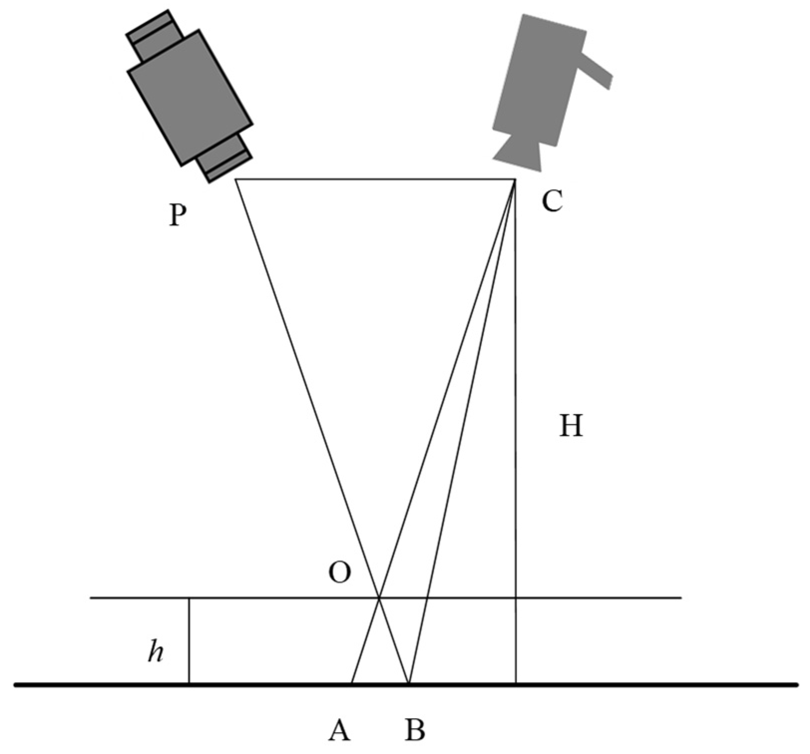
2.2. Principle of the DIP Measurement Technology

The basic principle of the DIP measurement technology is shown in Figure 2. The camera, the projection, and the experimental flat formed a triangular layout. The projector projected the grid image on the experimental flat before the start of the fluid flowing through it. Meanwhile, the camera collected the grid image as the reference image. When the fluid started flowing through the experimental flat, the grid image was projected on the fluid surface and deformed. The camera recorded the deformed grid as the experimental image. By analyzing the displacement of the corresponding points of the experimental image and the reference image, the three-dimensional shapes of the measured fluid could then be reconstructed. To convert the displacement of the corresponding points into the fluid thickness, the DIP system needed to be calibrated to establish the relationship between the thickness and the displacement.
As shown in Figure 2, the height of the camera from the reference plane was H and the height of water film was h . The camera lens C was taken as the origin, and the plane was parallel to the reference plane. Since Δ A B O is similar to Δ C P O , therefore:
h H h = A B ¯ C P ¯
As H > > h , the formula can be simplified to:
h = H h C P ¯ A B ¯ H C P ¯ A B ¯ = K A B ¯ ,
H and C P ¯ were taken as the constant values for a given optical system. Therefore, the thickness displacement conversion coefficient K was also constant with the unit of mm/pixel.
Based on the principle of thickness displacement conversion, the thickness can be converted to pixel displacement for both the experimental and reference images to accurately describe the motion behavior of the water film.

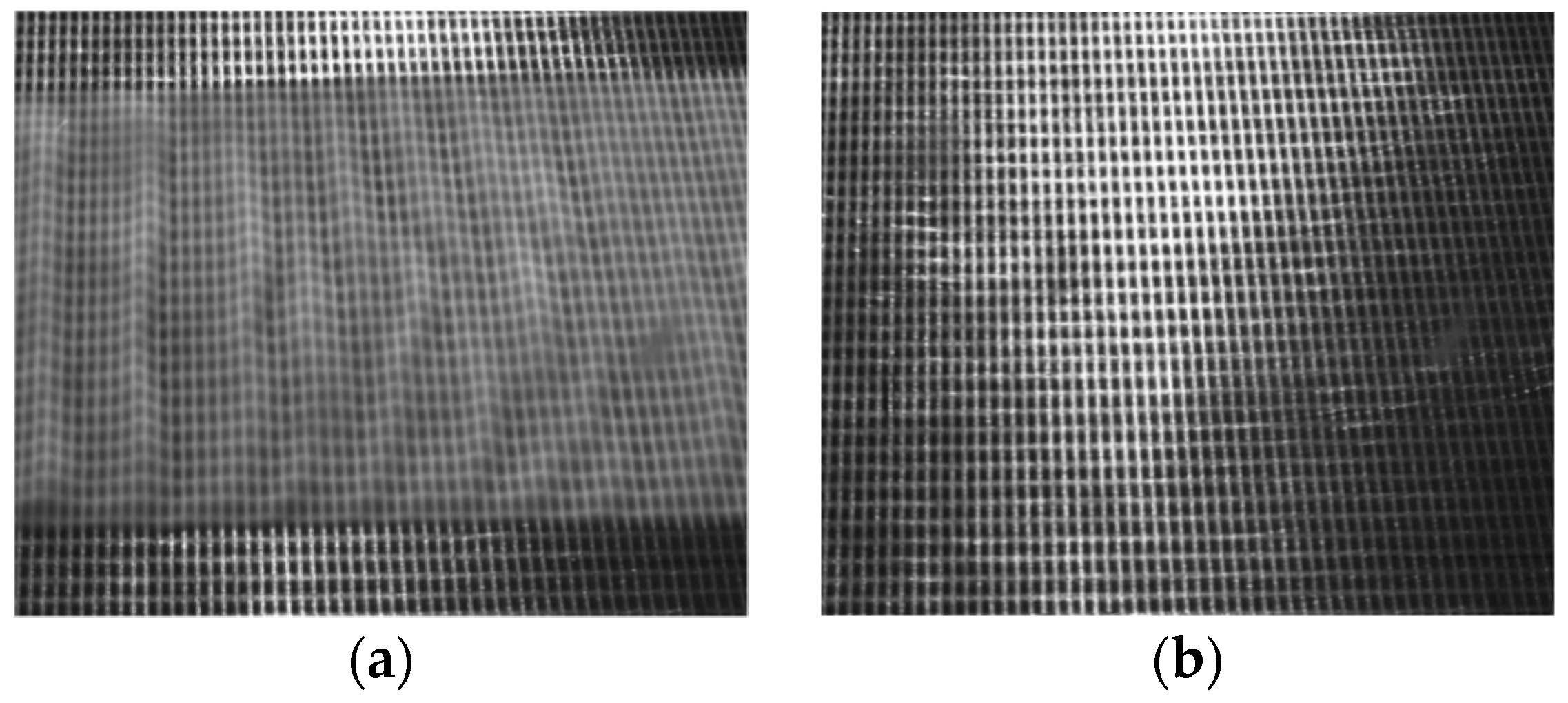
2.3. Calibration and Measurement of Experimental System

For a given DIP system, the displacement of the corresponding points in the experimental image and reference image changed linearly with the fluid thickness. Calibration of the DIP system can be used to determine the conversion coefficient K between the displacement of the experimental image and the reference thickness. The grid image was projected onto the experimental flat by the digital projection. The experimental flat was horizontally installed on the top of the lifting table, and its thickness was adjusted by a micron driver. The camera was used to capture the image projected on the experimental flat, and the obtained image was then stored on the computer for image processing.
In the process of the system calibration, by adjusting the thickness of the lifting table, the experimental flat was moved to multiple positions in the Y direction at certain intervals to obtain the grid image projected on the experimental flat. After that, the image was processed by using the image cross-correlation algorithm. Taking the image at Y = 0 as the reference image, the displacement of the focus points was calculated when the experimental flat was in other positions. In this way, the displacement value of the corresponding point could be obtained. The relationship between the thickness and the displacement of the corresponding point can be fitted by the linear function. The linear scale factor obtained in the calibration process was the K value of the DIP measurement system, and the K value was set as constant.
The experimental image was taken where the flat was restored to the Y = 0 origin, as shown in Figure 3a. A reference image is presented in Figure 3b. It can be observed that the surface grid of water film had moved.
For the accuracy of the calibrated DIP system, the thickness of the standard bench was measured using the system. The thickness of the table was 500 μm, and the platform was measured according to the experiment procedure previously mentioned. According to the measured results, the average thickness of the water film was 502.97 μm and the R M S f was 0.089. The experiment error was negligible compared to the measurement results of the experiment.

2.4. Measurement Results Processing Method

Dimensionless parameters were introduced to represent the flow rate of the water film. The Reynolds number of the water film, Re f is defined as:
Re f = Q L v l ,
where Q is the volume flow rate; L is the wetting width of the water film; and v l is the kinematic viscosity of the liquid.
Considering that the fluctuation intensity and randomness of the water film at different moments are different, the average value of the water film thickness at different times was taken as the experiment result.
For the measured range a b , the average thickness δ ¯ of the water film was defined as:
δ ¯ = 1 a b q = 1 b p = 1 a δ p q ,
where a and b are the total number of grid points of the horizontal and vertical coordinates of the selected grid area, respectively. δ p q is the thickness of the local water film at the grid point, and δ ¯ is the average of the thickness of the water film in the selected grid area. At least five repetitive tests were implemented to achieve the average thickness of the water film.
The fluctuation intensity of the water film was measured by defining the average root mean square R M S f of the liquid film extension direction for the grid area of the selected a b , which is defined as:
R M S f = 1 b q = 1 b [ 1 a p = 1 a ( δ p q δ q ¯ ) 2 ] 1 / 2 ,
where p is the flow direction of the water film; q is the direction perpendicular to p on the flat plate; δ q ¯ is the average thickness of the water film in line of q ; R M S f is the overall representation of the fluctuation of the water film in the direction of the selected grid region, omitting the error caused by the lateral tilt of the experimental bench.
Additionally, the average R M S f was achieved by at least five repetitive calculations.

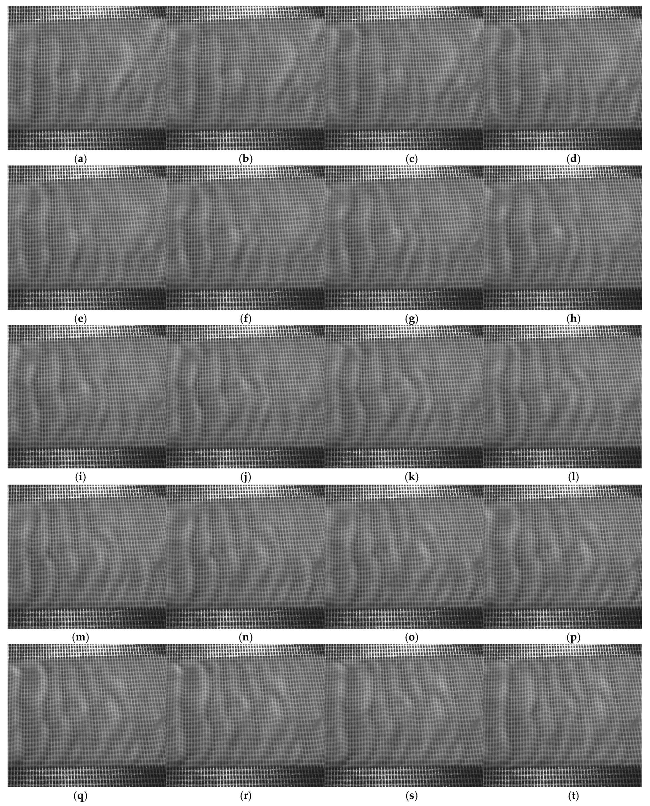
3. Results and Analysis

The whole process of the fluctuation transmission in the water film is shown in Figure 4. The fluctuation propagation of the water film flow was recorded using a high-speed camera to obtain the fluctuation velocity of the water film under different conditions. The sampling frequency of the camera was set at 100 Hz. The position of the fluctuation crest before and after the transmission along the direction of the water film flow in the grid was tracked and selected. The fluctuation transmission speed on the grid line was obtained by converting the selected pixel displacement into the actual flow distance and dividing it by the shooting interval. The final fluctuation velocity of the water film was obtained by calculating the transmission velocity of the fluctuation on each grid line and averaging it.

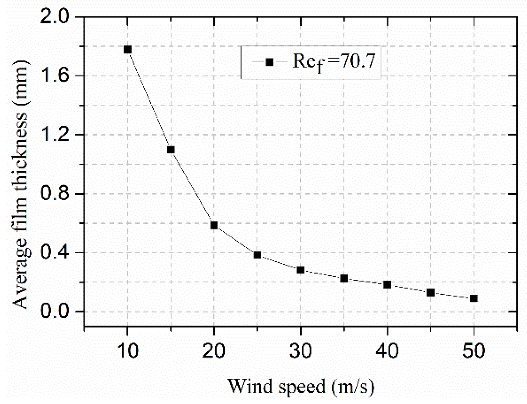
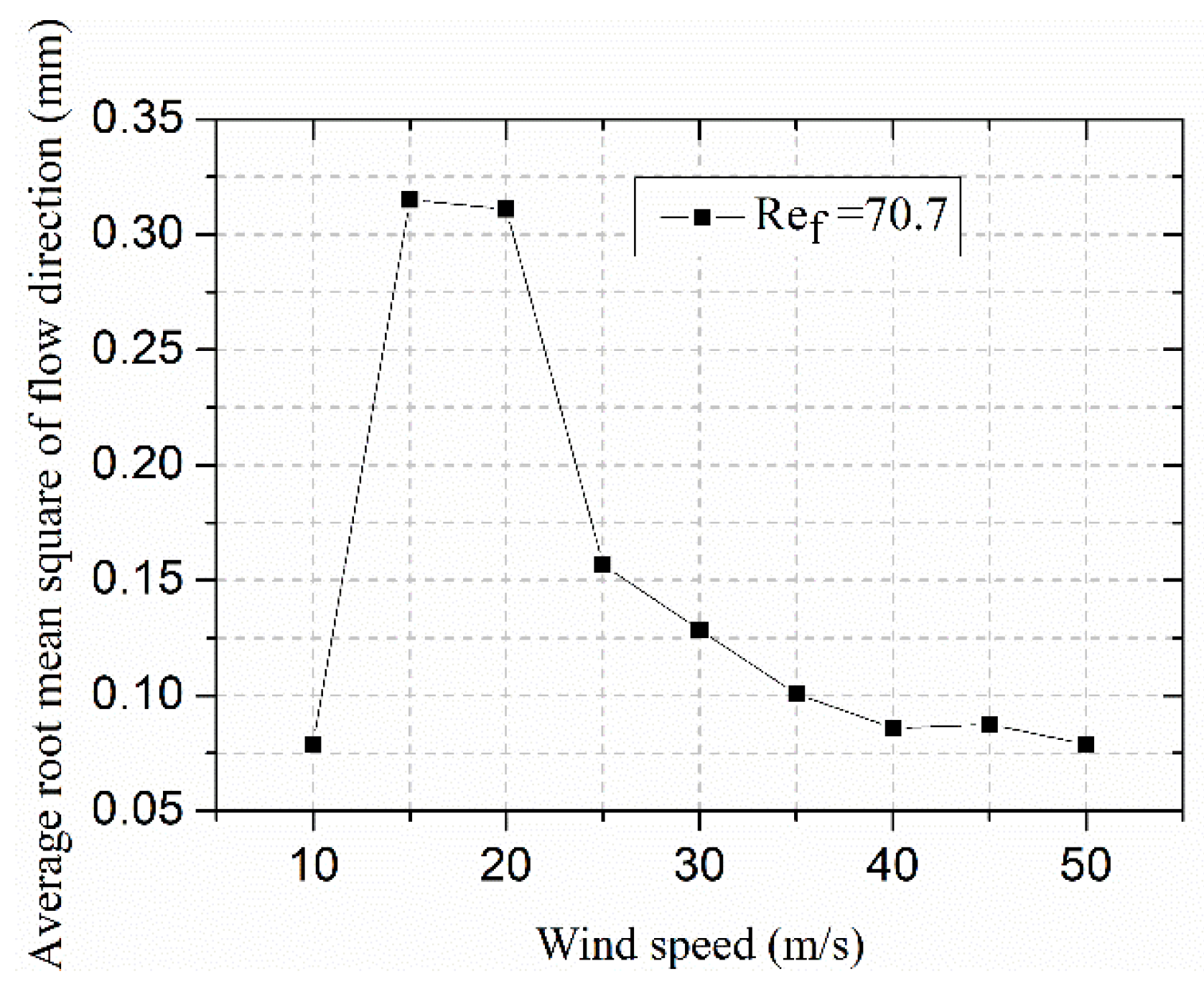
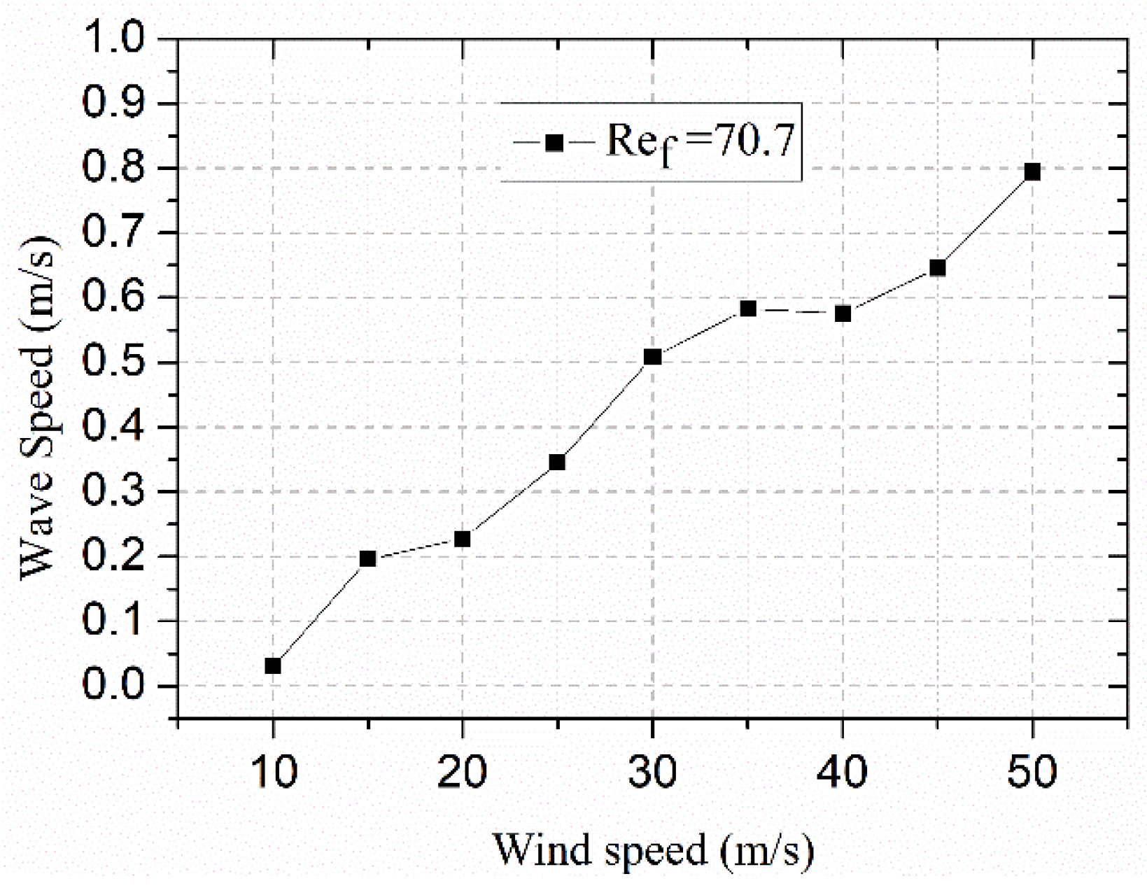
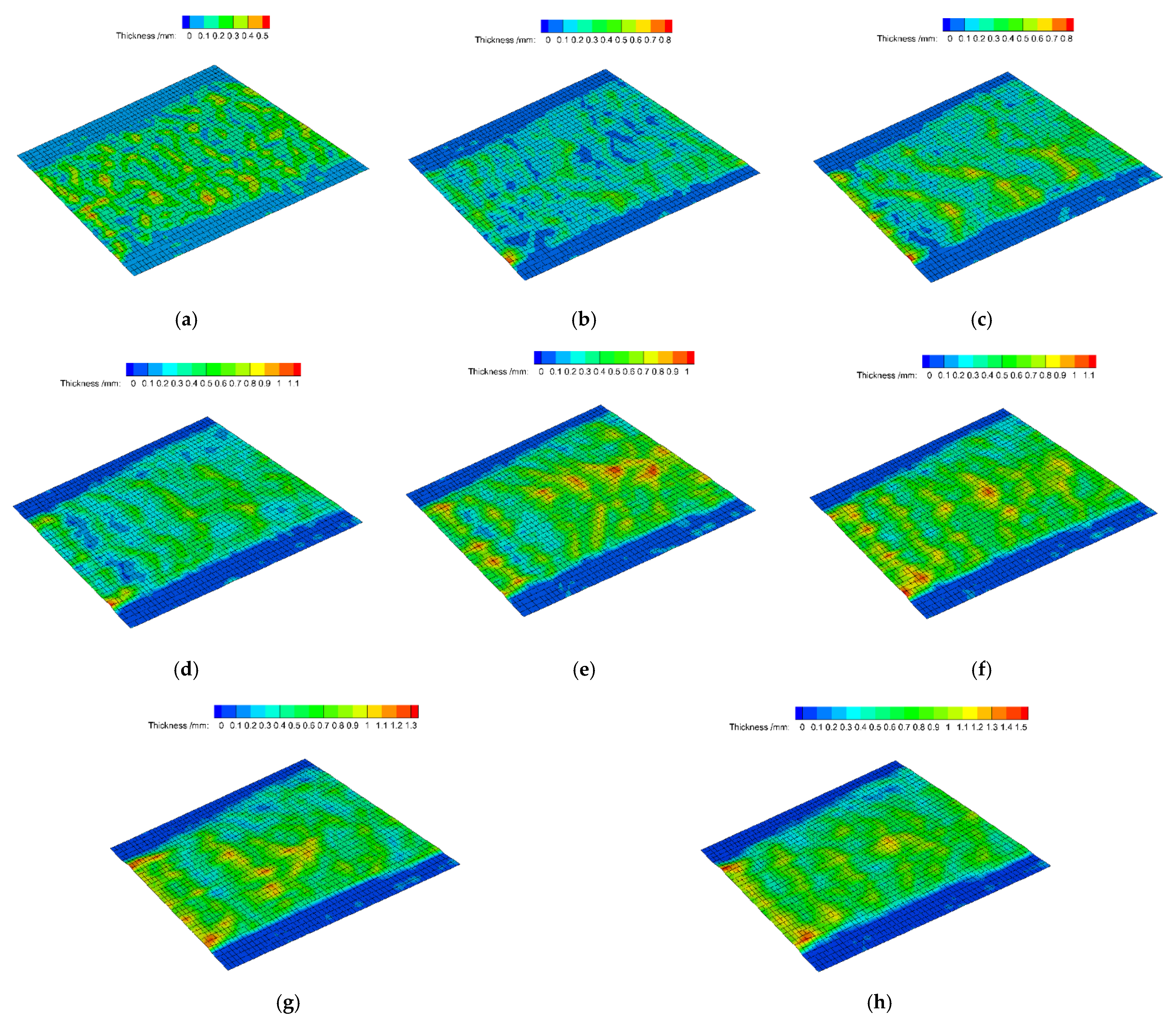
3.1. Effect of Wind Speed on the Water Film Flow

The Reynolds number of the water film was set at 70.7 to explore the influence of the wind speed on the film flow. Figure 5 displays the typical measurement results of the water film flow in the wind speed range of 10–50 m/s.
Figure 5a shows that the water film surface was very stable at the speed of 10 m/s. The reason for this phenomenon was that the surface tension of water was the dominant force at this time, and it resisted the influence of the airflow shear force on the gas–liquid interface. At the same instance, the average thickness of the water film δ ¯ was the largest. However, the R M S f value representing the surface fluctuation intensity was the smallest as the surface fluctuation was very weak. Similarly, the fluctuation velocity was also found to be very small.
When the speed increased to 15 m/s, a rolling fluctuation with a large amplitude and small frequency was formed at the gas–liquid interface under the combined action of the surface tension and airflow shear force, as shown in Figure 5b. This occurred because of the enhanced influence of the airflow shear force. As the surface tension still played a strong role, the small-scale clutter had not yet appeared. Meanwhile, the average thickness of the water film δ ¯ decreased rapidly, the R M S f value increased significantly, and a gradual increase was observed in the fluctuation velocity.
As shown in Figure 5c, when V = 20 m/s, further enhancement could be spotted in the influence of the shear force, whereas the frequency of gas–liquid interface fluctuation significantly increased. Under the action of the surface tension, the water film interfacial fluctuation could essentially maintain the transverse integrity. In the meantime, the average water film thickness δ ¯ continued to drastically decrease. However, the R M S f value remained at a high level with the gradual increase in the fluctuation velocity.
At V = 25 m/s, the effect of the shear force on the water film movement slowly increased while there was a further decrease in the influence of the surface tension. The interface fluctuation could be transversely integrated near the leading-edge outlet of the water film, and gradually decomposed into the multisequence clutter in the mid-stage. Figure 5 clearly shows that the water film at this instance is close to the flat surface at the trough. The larger amplitude of the interfacial fluctuation could clearly not be maintained, and the influence of the lower surface on the flow of the water film was enhanced. The average thickness of the water film δ ¯ started to decrease slowly. The R M S f value, which represents the strength of the fluctuation, also showed a rapid drop with the continued rise in the fluctuation velocity.
As shown in Figure 5e–h, when V = 30–45 m/s, a similar flow pattern of the water film was observed in this region. However, it broke into tiny clutters once the water film flowed out of the outlet. As the velocity increased, the clutters became smaller. Since the water film was very thin, the water film near the viscous bottom was not in its peak position. The water fluctuations indicated a rapid movement of the isolated peaks on the wet surface. With the increase in the velocity, the average thickness δ ¯ of the water film showed a linear downward trend, while both the moving peak and the R M S f value decreased gradually. However, due to the similarity in the water film flow law, the variation in the fluctuation velocity was not significant in this range.
The water film was still very thin at V = 50 m/s, especially in the nonpeak position. Therefore, it could only maintain the continuous wet environment on the surface of the experimental piece. Under the action of the high-speed airflow, water fluctuations formed isolated and tiny droplets. Due to the surface tension of the water at this point, the droplets propagated faster on the wet surfaces while withstanding the aerodynamic forces. Consequently, the fluctuation velocity increased significantly in this state.
Figure 5, Figure 6, Figure 7 and Figure 8 show that when the Reynolds number of the water film was 70.7, the influence of the wind speed on the flow of the water film could be divided into three stages. In the first stage, the wind speed was 10–25 m/s. The influence of the lower surface on the surface fluctuation of the water film was limited, but the surface tension of the water had a great influence on it. With the increase in the wind speed, a significant drop was observed in the average thickness δ ¯ of the water film. Additionally, the R M S f value representing the fluctuation intensity initially increased and then decreased, whereas the fluctuation velocity increased steadily. In the second stage, when the wind speed was 30–45 m/s, the water film became reasonably thin. The impact of the lower wall on the surface of the water film was very large. The water film at the nonpeak was found to be close to the viscous bottom. The surface fluctuation of the water film was more like isolated clutters sliding on a wet surface. In this interval, unnoticeable variation was observed in the fluctuation velocity. In the third stage, the wind speed was greater than 50 m/s. Small clutter peaks became small moving droplets under the action of the surface tension of the water. The fluctuation velocity increased significantly under the aerodynamic action.
In this experiment, the Reynolds number of the water film was calculated as 70.7. This Reynolds number helped in the better characterization of the variation in the gas–liquid interface fluctuation in each stage under the limited wind speed range. Otherwise, it was necessary to expand the experimental wind speed range to obtain similar results if the Reynolds number of the water film was increased.

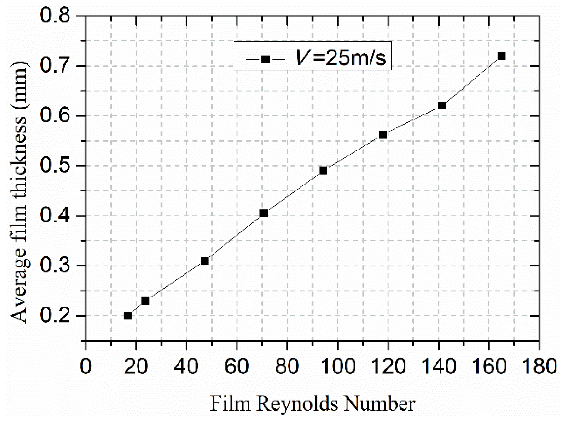
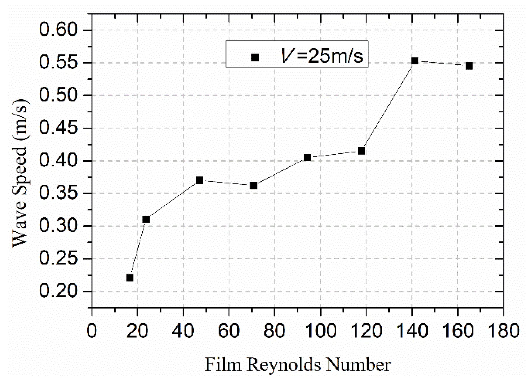
3.2. Effect of Reynolds Number on the Water Film Flow

As shown in Figure 9, when Re f = 16.5–23.6, the water flow at this time was too small at the same speed. The average thickness of the water film was also very small. The lower wall had a greater influence on the fluctuation of the water film. Therefore, it was impossible to maintain a large fluctuation intensity, resulting in a lower R M S f value. Within this interval, a small increase in Re f resulted in a substantial increase in the fluctuation velocity.
When Re f = 47.1–117.9, the average thickness of the water film increased linearly with the increase in Re f . Under the combined action of the surface tension of the water and the shear force of the airflow, a complete transverse fluctuation was formed on the surface of the water film and was transmitted in the backward direction. As the thickness of the water film was sufficient to satisfy the fluctuation transmission at the corresponding speed, the R M S f value remained small in an interval. No major variation was observed in the fluctuation transmission speed.
When Re f = 141.4–165.0, the average thickness of the water film continued to increase with the increase in Re f . The influence of the lower wall on the gas–liquid surface fluctuation was weakened. Meanwhile, the increasing water flow rate made the thick water film exhibit obvious turbulent characteristics under the action of the shearing force of the airflow. Furthermore, the fluctuation amplitude of the water film also remarkably increased. The water–film interface exhibited a distinct rolling fluctuation morphology, and the R M S f value and fluctuation transmission velocity also increased significantly.
When the wind speed was 25 m/s, the Reynolds number of the water film and the average thickness exhibited a linear growth relationship, as observed in Figure 10, Figure 11 and Figure 12. The variation in the wave structure was mainly divided into three stages. In the water film at a low Reynolds number (approx. 20), the wave strength and the wave velocity were found to be very small. In the water film at a medium Reynolds number (40–120) interval, the wave was fully developed and the fluctuation intensity and the wave velocity change were gentle. However, in the water film at high Reynolds number (140–160), the wave amplitude increased significantly, forming a distinct rolling wave, and the fluctuation intensity and wave speed were also substantially increased.
Using the method in [15] to process the experiment results in this paper, the relationship between the dimensionless height and Reynolds number can be obtained as h + = 1.3973 Re f 0.5689 . Compared to the values obtained by Leng and Kosky [15], the error between them was within the acceptable range.
The wettability also had an effect on the water film flow. In this paper, the water film flow experiment was carried out using conventional materials, so the water film flow process was continuous without breaking. Fluctuating characteristics and flow characteristics of the water film motion can be observed. When a superhydrophobic material was used as the surface, the contact angle of the surface became large and the water film could not completely cover the surface. In the low flow state, the water film thickness was thicker and clustered due to the weak airflow shear force. After the wind speed gradually increased, the airflow shear force was enhanced, and the water film on the superhydrophobic surface could only maintain a small continuous water film at the initial position, which will break rapidly during the development process. Therefore, the flow characteristics of the water film on the surface of different materials can vary greatly, and the flow characteristics of the water film on the surface of aluminum was studied in this paper.

4. Conclusions

In this paper, the flow process of the water film on the flat was observed using the digital image projection measurement system. The fluctuation characteristics of the water film under different wind speeds were obtained. The fluctuation structure of the water–air interface was deeply examined. It was found that when the Reynolds number of the water film was 70 or the wind speed was 25 m/s, the influence of the wind speed and Reynolds number on the fluctuation structure could be divided into three stages. When the Reynolds number of the water film was 70.7 and the wind speed was 50 m/s, droplets moved at a high speed on the surface. This study has a certain significance for understanding the microphysical process of anti-icing. In this paper, the flow characteristics of the water film on the surface of conventional materials were studied, and further research on the flow of the water film on the surface of superhydrophobic materials will be carried out.

Author Contributions

Conceptualization, H.Z., H.D., D.Z., N.Z., C.Z. (Chengxiang Zhu), S.L. and C.Z. (Chunling Zhu); Methodology, C.Z. (Chunling Zhu), N.Z. and C.Z. (Chengxiang Zhu); Validation, H.Z.; Formal analysis, H.Z. and H.D.; Resources, C.Z. (Chunling Zhu); Data curation, H.Z.; Writing—original draft preparation, H.Z., H.D. and D.Z.; Writing—review and editing, H.Z. and D.Z.; Project administration, C.Z. (Chunling Zhu); Funding acquisition, C.Z. (Chunling Zhu) and S.L. All authors have read and agreed to the published version of the manuscript.

Funding

This research was funded by the Open Fund of Key Laboratory of Icing and Anti/De-icing (Grant No. IADL20200107).

Institutional Review Board Statement

Not applicable.

Informed Consent Statement

Not applicable.

Data Availability Statement

The data presented in this study are available on request from the corresponding author.

Conflicts of Interest

The authors declare no conflict of interest.

References

  1. Dai, H.; Zhu, C.; Zhao, H.; Liu, S. A New Ice Accretion Model for Aircraft Icing Based on Phase-Field Method. Appl. Sci. 2021, 11, 5693. [Google Scholar] [CrossRef]
  2. Wang, Z.; Zhao, H.; Liu, S. Numerical Simulation of Aircraft Icing under Local Thermal Protection State. Aerospace 2022, 9, 84. [Google Scholar] [CrossRef]
  3. Holl, M.; Pátek, Z.; Smrcek, L. Wind Tunnel Testing of Performance Degradation of Ice Contaminated Airfoils. In Proceedings of the 22nd International Congress of Aeronautical Sciences, Harrogate, UK, 27 August–1 September 2000. [Google Scholar]
  4. Otta, S.P.; Rothmayer, A.P. Instability of Stagnation Line Icing. Comput. Fluids 2009, 38, 273–283. [Google Scholar] [CrossRef]
  5. Rothmayer, A.P.; Hu, H. Linearized Solutions of Three-Dimensional Condensed Layer Films. In Proceedings of the 5th AIAA Atmospheric and Space Environments Conference, AIAA, San Diego, CA, USA, 24–27 June 2013. [Google Scholar]
  6. Rothmayer, A.P.; Matheis, B.D.; Timoshin, S.N. Thin Liquid Films Flowing over External Aerodynamic Surfaces. J. Eng. Math. 2002, 42, 341–357. [Google Scholar] [CrossRef]
  7. Wang, G.; Rothmayer, A.P. Thin Water Films Driven by Air Shear Stress Through Roughness. Comput. Fluids 2009, 38, 235–246. [Google Scholar] [CrossRef]
  8. Planquart, P.; Riethmuller, M.; Joly, A.; Detry, J.M. Real Time Optical Detection and Characterisation of Water Model Free Surfaces—Application to the Study of the Mold. In Proceedings of the 4th European Continuous Casting Conference, Birmingham, UK, 14–16 October 2002. [Google Scholar]
  9. Touron, F.; Labraga, L.; Keirsbulck, L.; Bratec, H. Measurements of Liquid Film Thickness of a Wide Horizontal Co-current Stratified Air-Water Flow. Therm. Sci. 2015, 19, 521–530. [Google Scholar] [CrossRef]
  10. Cherdantsev, A.V.; Hann, D.B.; Azzopardi, B.J. Study of Gas-Sheared Liquid Film in Horizontal Rectangular Duct Using High-Speed LIF Technique: Three-Dimensional Wavy Structure and Its Relation to Liquid Entrainment. Int. J. Multiph. Flow 2014, 67, 52–64. [Google Scholar] [CrossRef]
  11. Zhang, K.; Zhang, S.; Rothmayer, A.P.; Hu, H. Development of a Digital Image Projection Technique to Measure Wind-Driven Water Film Flows. In Proceedings of the 51st AIAA Aerospace Sciences Meeting AIAA, Grapevine, TX, USA, 7–10 January 2013. [Google Scholar]
  12. Zhang, K.; Blake, J.; Rothmayer, A.P.; Hu, H. An Experimental Investigation on Wind-Driven Rivulet/Film Flows over a NACA0012 Airfoil by Using Digital Image Projection Technique. In Proceedings of the 52nd Aerospace Sciences Meeting, AIAA, National Harbor, MD, USA, 13–17 January 2014. [Google Scholar]
  13. Zhang, K.; Tian, W.; Hu, H. An Experimental Investigation on the Surface Water Transport Process over an Airfoil by Using a Digital Image Projection Technique. Exp. Fluids 2015, 56, 173. [Google Scholar] [CrossRef]
  14. Chang, S.; Yu, W.; Song, M.; Leng, M.; Shi, Q. Investigation on Wavy Characteristics of Shear-Driven Water Film Using the Planar Laser Induced Fluorescence Method. Int. J. Multiph. Flow 2019, 118, 242–253. [Google Scholar]
  15. Leng, M.; Chang, S.; Wu, H. Experimental Investigation of Shear-Driven Water Film Flows on Horizontal Metal Plate. Exp. Therm. Fluid Sci. 2018, 94, 134–147. [Google Scholar] [CrossRef] [Green Version]
  16. Zhao, H.; Zhu, C.; Zhao, N.; Zhu, C.; Wang, Z. Experimental Research on the Influence of Roughness on Water Film Flow. Aerospace 2021, 8, 225. [Google Scholar] [CrossRef]
Figure 1. The water film measurement system [16].
Coatings 12 01040 g001
Figure 2. The optical principle of the thickness position conversion.
Coatings 12 01040 g002
Figure 3. The optical principle of the thickness position conversion: (a) experimental image; (b) reference image.
Coatings 12 01040 g003
Figure 4. Images of the water film flow experiments at (a) t = 0 s; (b) t = 0.01 s; (c) t = 0.02 s; (d) t = 0.03 s; (e) t = 0.04 s; (f) t = 0.05 s; (g) t = 0.06 s; (h) t = 0.07 s; (i) t = 0.08 s; (j) t = 0.09 s; (k) t = 0.1 s; (l) t = 0.11 s; (m) t = 0.12 s; (n) t = 0.13 s; (o) t = 0.14 s; (p) t = 0.15 s; (q) t = 0.16 s; (r) t = 0.17 s; (s) t = 0.18 s; (t) t = 0.19 s.
Coatings 12 01040 g004
Figure 5. The images of the water film flow experiments at (a) V = 10 m/s; (b) V = 15 m/s; (c) V = 20 m/s; (d) V = 25 m/s; (e) V = 30 m/s; (f) V = 35 m/s; (g) V = 40 m/s; (h) V = 45 m/s; (i) V = 50 m/s.
Coatings 12 01040 g005
Figure 6. The variation in the wind velocity and the average water film thickness.
Coatings 12 01040 g006
Figure 7. The variation in the wind speed and RMSf.
Coatings 12 01040 g007
Figure 8. The variation in the wind and fluctuation velocity of the water film.
Coatings 12 01040 g008
Figure 9. The DIP measurements at 25 m/s wind speed: (a) Re f = 16.5; (b) Re f = 23.6; (c) Re f =47.1; (d) Re f = 70.7; (e) Re f = 94.3; (f) Re f = 117.9; (g) Re f = 141.4; (h) Re f = 165.
Coatings 12 01040 g009
Figure 10. The variation in the Reynolds number and the average thickness of the water film.
Coatings 12 01040 g010
Figure 11. The variation in the Reynolds number of the water film and RMSf.
Coatings 12 01040 g011
Figure 12. The variation in the Reynolds number and fluctuation velocity of the water film.
Coatings 12 01040 g012
Publisher’s Note: MDPI stays neutral with regard to jurisdictional claims in published maps and institutional affiliations.

