
Tunable Coefficient of Thermal Expansion of Composite Materials for Thin-Film Coatings


Abstract
:1. Introduction
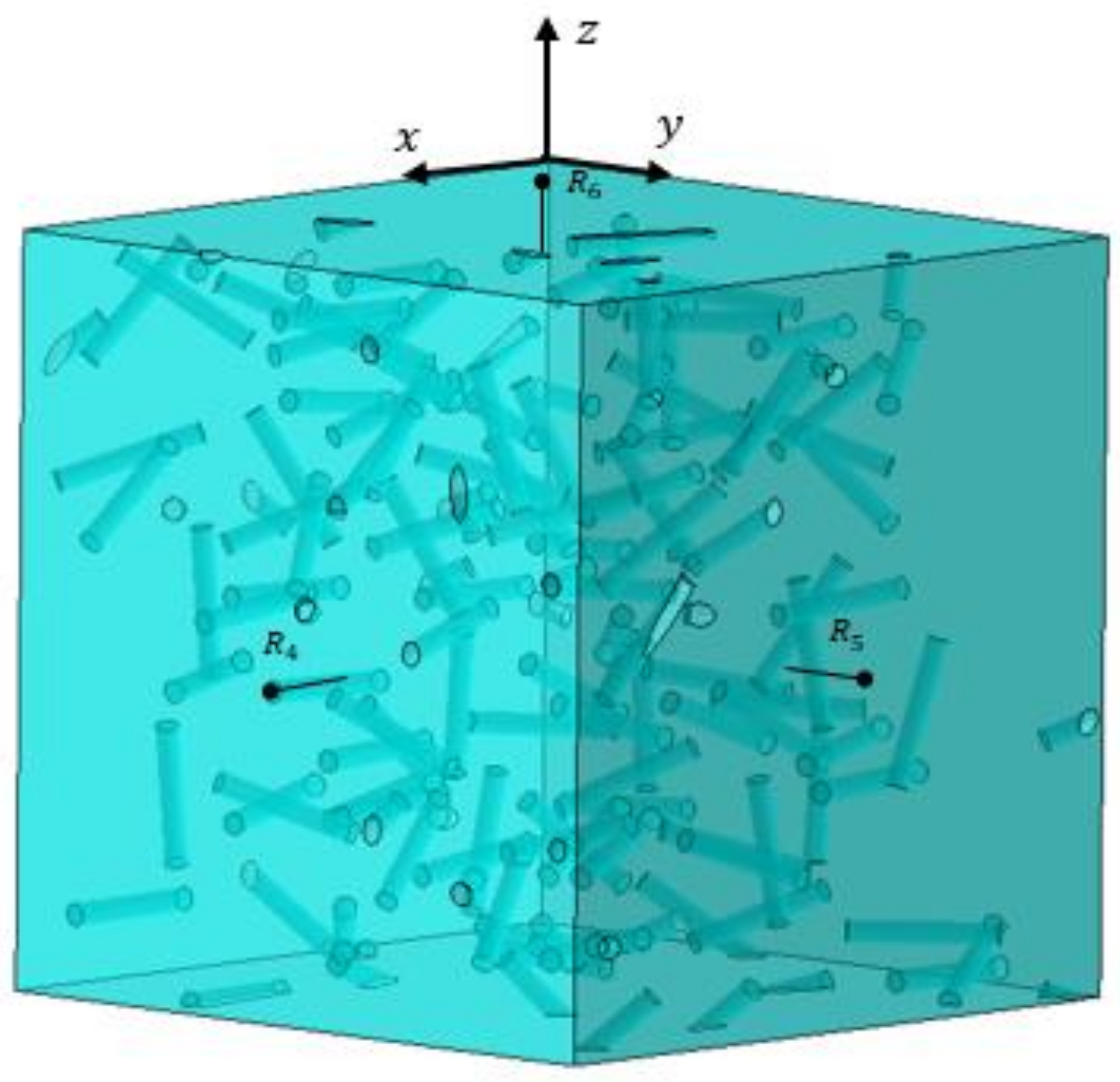
- A simulation model of RVEs is established based on the theory of mesomechanics, and the process and difficulties of its establishment are described in detail.
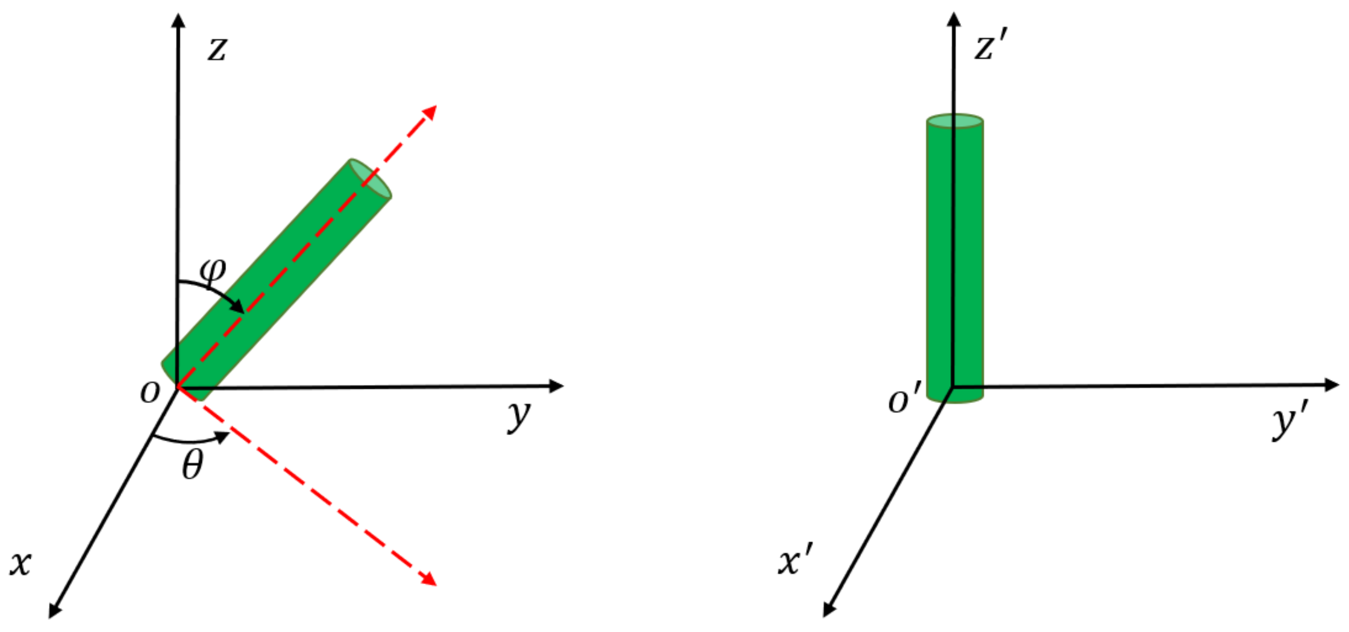
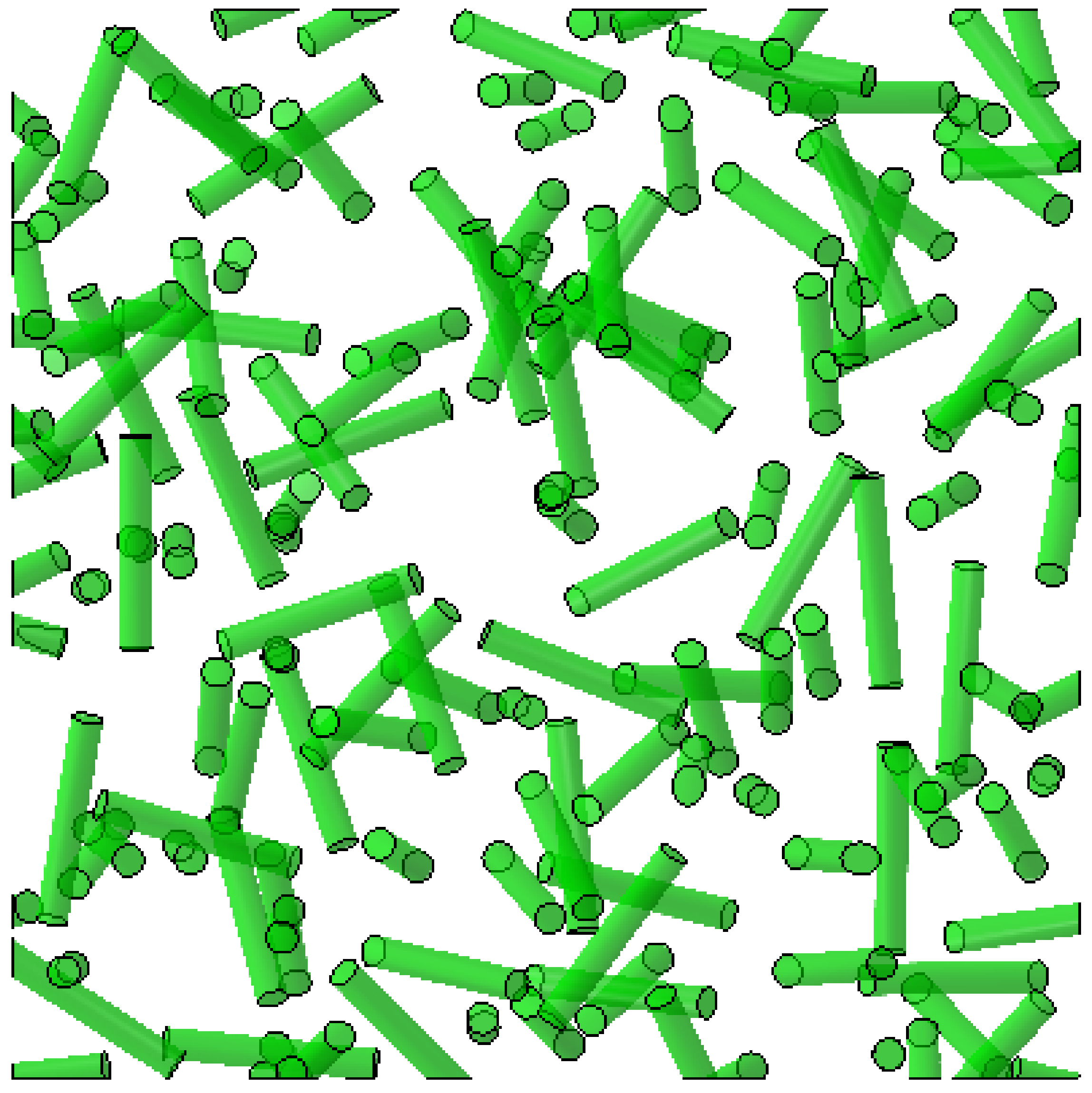
- The random distribution of the position and direction of the fiber material in the composite materials for thin-film coatings is realized by the calculation method combined with the relevant development script file of ABAQUS.
- The close integration of periodic boundary condition theory and finite element simulation software is realized, and constraints are imposed on the corresponding nodes of the RVEs.
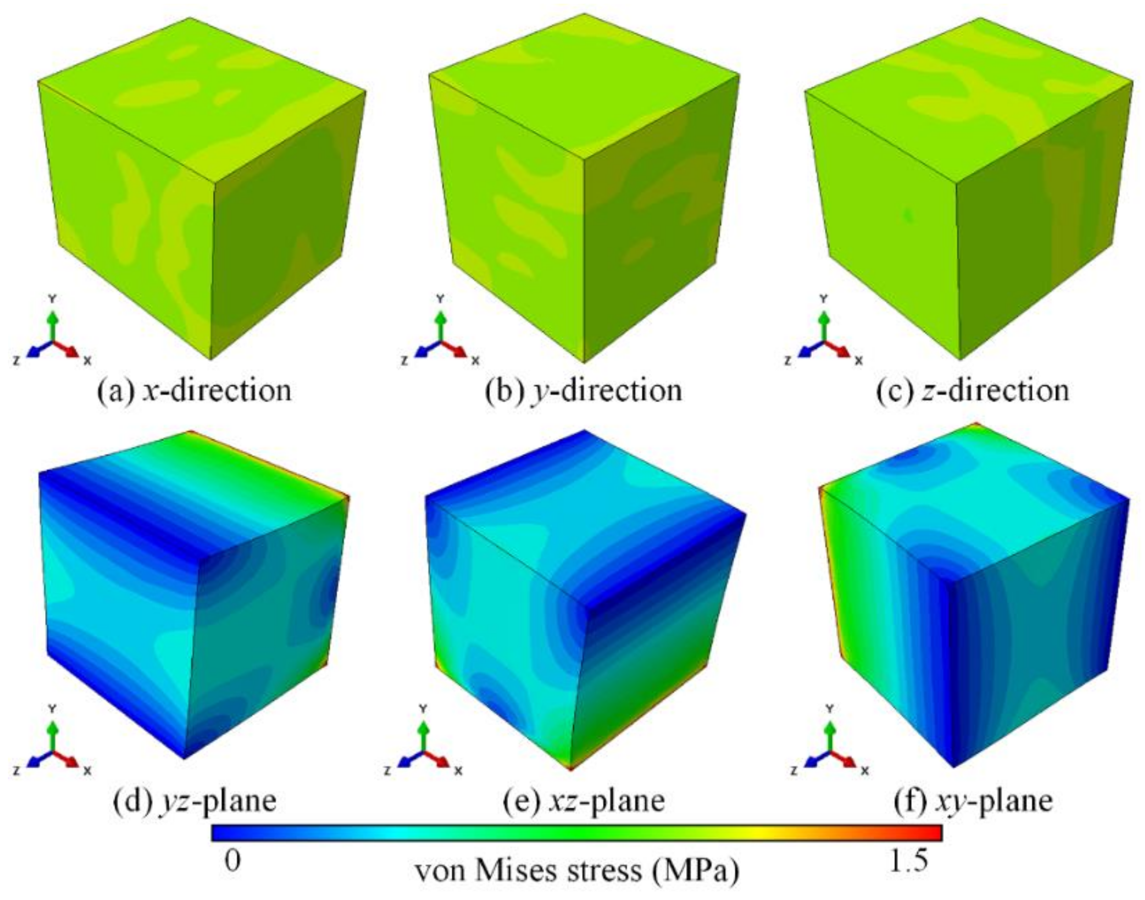
- The macroscopic mechanical properties and CTE in RVEs are calculated based on the randomness of the fiber distribution.
2. Modeling of Representative Volume Elements for Composite Materials
2.1. Representative Volume Element Design Steps
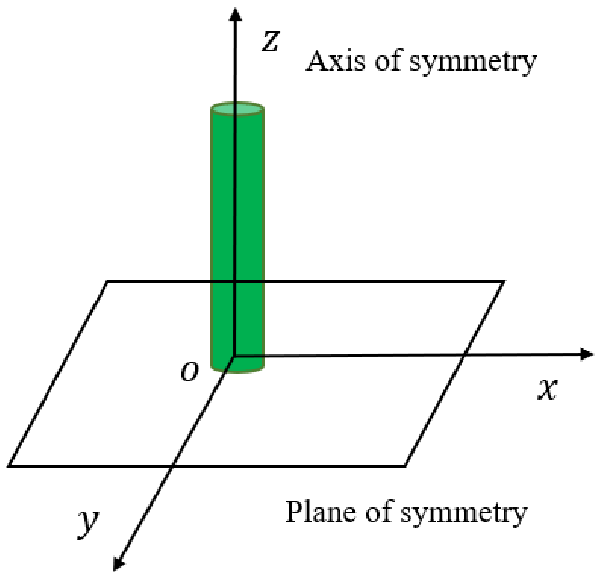
2.2. Periodic Boundary Conditions for the RVE
3. Equivalent CTE of Representative Volume Elements
4. Result Discussion
5. Conclusions
- The mesomechanical modeling of fiber-reinforced matrix composites is complex, involving the random distribution and random orientation of fibers. In this paper, the parametric modeling method based on Python program script files was used to improve modeling efficiency significantly.
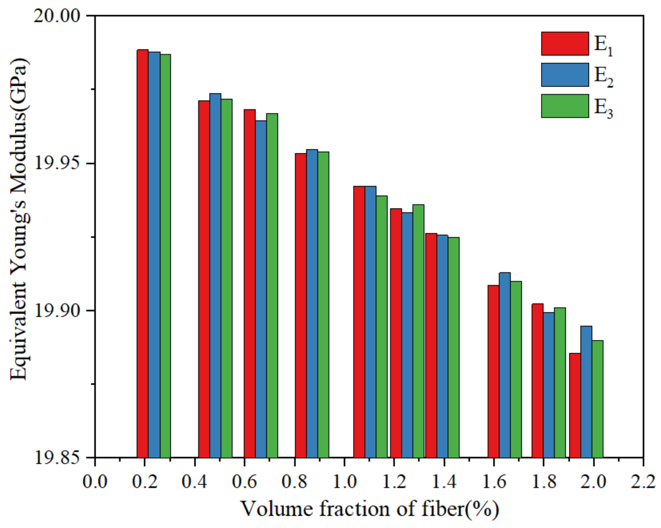
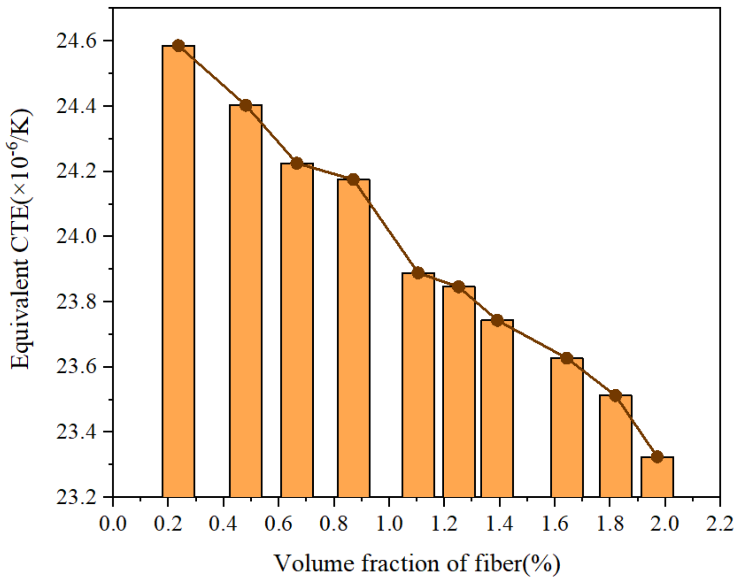
- Through the finite element analysis of the fiber-reinforced matrix composite material model, it was found that the equivalent thermal expansion coefficient of the material can be effectively reduced with the continuous increase in the fiber volume fraction.
Author Contributions
Funding
Institutional Review Board Statement
Informed Consent Statement
Data Availability Statement
Conflicts of Interest
References
- Zeng, Q.; Yu, A.; Lu, G.M. Interfacial interactions and structure of polyurethane intercalated nanocomposite. Nanotechnology 2005, 16, 2757. [Google Scholar] [CrossRef]
- Hashimoto, M.; Okabe, T.; Sasayama, T.; Matsutani, H.; Nishikawa, M. Prediction of tensile strength of discontinuous carbon fiber/polypropylene composite with fiber orientation distribution. Compos. Part A Appl. Sci. Manuf. 2012, 43, 1791–1799. [Google Scholar] [CrossRef]
- Kwon, D.J.; Jang, Y.J.; Choi, H.H.; Kim, K.; Kim, G.H.; Kong, J.; Nam, S.Y. Impacts of thermoplastics content on mechanical properties of continuous fiber-reinforced thermoplastic composites. Compos. Part B Eng. 2021, 216, 108859. [Google Scholar] [CrossRef]
- Lee, J.Y.; Baljon, A.; Loring, R.F.; Panagiotopoulos, A.Z. Simulation of polymer melt intercalation in layered nanocomposites. J. Chem. Phys. 1998, 109, 10321–10330. [Google Scholar] [CrossRef]
- Smith, G.D.; Bedrov, D.; Li, L.W.; Byutner, O. A molecular dynamics simulation study of the viscoelastic properties of polymer nanocomposites. J. Chem. Phys. 2002, 117, 9478–9489. [Google Scholar] [CrossRef]
- Thompson, R.B.; Ginzburg, V.V.; Matsen, M.W.; Balazs, A.C. Block copolymer-directed assembly of nanoparticles: Forming mesoscopically ordered hybrid materials. Macromolecules 2002, 35, 1060–1071. [Google Scholar] [CrossRef]
- Panin, V.E. Physical Mesomechanics of Heterogeneous Media and Computer-Aided Design of Materials; Cambridge International Science Publishing: Cambridge, UK, 1998. [Google Scholar]
- Mishnaevsky, L.L., Jr.; Schmauder, S. Contimuum mesomechanical finite element modeling in materials development: A state-of-the-art review. Adv. Mech. 2002, 54, 49. [Google Scholar]
- Long, X.; Guo, Y.; Chang, X.; Su, Y.; Shi, H.; Huang, T.; Tu, B.; Wu, Y. Effect of Temperature on the Fatigue Damage of SAC305 Solder. In Proceedings of the 2021 22nd International Conference on Electronic Packaging Technology (ICEPT), Xiamen, China, 14–17 September 2021; pp. 1–4. [Google Scholar]
- Long, X.; Su, T.; Chang, C.; Huang, J.; Chang, X.; Su, Y.; Shi, H.; Huang, T.; Wu, Y. Mechanical Behavior of Lead-Free Solder at High Temperatures and High Strain Rates. In Proceedings of the 2021 22nd International Conference on Electronic Packaging Technology (ICEPT), Xiamen, China, 14–17 September 2021; pp. 1–4. [Google Scholar]
- Andriyana, A.; Billon, N.; Silva, L. Mechanical response of a short fiber-reinforced thermoplastic: Experimental investigation and continuum mechanical modeling. Eur. J. Mech. A Solids 2010, 29, 1065–1077. [Google Scholar] [CrossRef]
- Wan, Y.; Takahashi, J. Tensile properties and aspect ratio simulation of transversely isotropic discontinuous carbon fiber reinforced thermoplastics. Compos. Sci. Technol. 2016, 137, 167–176. [Google Scholar] [CrossRef]
- Mirkhalaf, S.M.; Eggels, E.H.; van Beurden, T.J.H.; Larsson, F.; Fagerström, M. A finite element based orientation averaging method for predicting elastic properties of short fiber reinforced composites. Compos. Part B Eng. 2020, 202, 108388. [Google Scholar] [CrossRef]
- Díaz, A.R.; Flores, E.I.S.; Yanez, S.J.; Vasco, D.A.; Pina, J.C.; Guzmán, C.F. Multiscale modeling of the thermal conductivity of wood and its application to cross-laminated timber. Int. J. Therm. Sci. 2019, 144, 79–92. [Google Scholar] [CrossRef]
- Trzepieciński, T.; Ryzińska, G.; Biglar, M.; Gromada, M. Modelling of multilayer actuator layers by homogenisation technique using Digimat software. Ceram. Int. 2016, 43, 3259–3266. [Google Scholar] [CrossRef]
- Chao, X.J.; Qi, L.H.; Tian, W.L.; Lu, Y.F.; Li, H.J. Potential of porous pyrolytic carbon for producing zero thermal expansion coefficient composites: A multi-scale numerical evaluation. Compos. Struct. 2020, 235, 111819. [Google Scholar] [CrossRef]
- Miller, W.; Hook, P.B.; Smith, C.W.; Wang, X.; Evans, K.E. The manufacture and characterisation of a novel, low modulus, negative Poisson’s ratio composite. Compos. Sci. Technol. 2009, 69, 651–655. [Google Scholar] [CrossRef]
- Sun, Z.; Shan, Z.D.; Shao, T.M.; Li, J.H.; Wu, X.C. A multiscale modeling for predicting the thermal expansion behaviors of 3D C/SiC composites considering porosity and fiber volume fraction. Ceram. Int. 2021, 47, 7925–7936. [Google Scholar] [CrossRef]
- Wei, K.; Peng, Y.; Wang, K.Y.; Duan, S.Y.; Yang, X.J.; Wen, W.B. Three dimensional lightweight lattice structures with large positive, zero and negative thermal expansion. Compos. Struct. 2018, 188, 287–296. [Google Scholar] [CrossRef]
- Liu, H.; Zeng, D.; Li, Y.; Jiang, L.Y. Development of RVE-embedded solid elements model for predicting effective elastic constants of discontinuous fiber reinforced composites. Mech. Mater. 2016, 93, 109–123. [Google Scholar] [CrossRef]
- Kobayashi, S.; Shimpo, T.; Goto, K. Microscopic damage behavior in carbon fiber reinforced plastic laminates for a high accuracy antenna in a satellite under cyclic thermal loading. Adv. Compos. Mater. 2019, 28, 259–269. [Google Scholar] [CrossRef]
- Hao, X.L.; Zhou, H.Y.; Mu, B.S.; Chen, L.; Guo, Q.; Yi, X.; Sun, L.C.; Wang, Q.W.; Ou, R.X. Effects of fiber geometry and orientation distribution on the anisotropy of mechanical properties, creep behavior, and thermal expansion of natural fiber/HDPE composites. Compos. Part B Eng. 2020, 185, 107778. [Google Scholar] [CrossRef]
- Gu, J.P.; Leng, J.S.; Sun, H.Y.; Zeng, H.; Cai, Z.B. Thermomechanical constitutive modeling of fiber reinforced shape memory polymer composites based on thermodynamics with internal state variables. Mech. Mater. 2019, 130, 9–19. [Google Scholar] [CrossRef]
- Sun, Q.P.; Zhou, G.W.; Meng, Z.X.; Jain, M.; Su, X.M. An integrated computational materials engineering framework to analyze the failure behaviors of carbon fiber reinforced polymer composites for lightweight vehicle applications. Compos. Sci. Technol. 2021, 202, 108560. [Google Scholar] [CrossRef]
- Chen, L.L.; Gu, B.Q.; Zhou, J.F.; Tao, J.H. Study of the effectiveness of the RVEs for random short fiber reinforced elastomer composites. Fibers Polym. 2019, 20, 1467–1479. [Google Scholar] [CrossRef]
- Naili, C.; Doghri, I.; Kanit, T.; Sukiman, M.S.; Aissa-Berraies, A.; Imad, A. Short fiber reinforced composites: Unbiased full-field evaluation of various homogenization methods in elasticity. Compos. Sci. Technol. 2020, 187, 107942. [Google Scholar] [CrossRef]
- Garoz, D.; Gilabert, F.A.; Sevenois, R.D.B.; Spronk, S.W.F.; Van Paepegem, W. Consistent application of periodic boundary conditions in implicit and explicit finite element simulations of damage in composites. Compos. Part B Eng. 2019, 168, 254–266. [Google Scholar] [CrossRef]
- Chen, L.; Tao, X.M.; Choy, C.L. Mechanical analysis of 3-D braided composites by the finite multiphase element method. Compos. Sci. Technol. 1999, 59, 2383–2391. [Google Scholar] [CrossRef]
- Suquet, P. Elements of homogenization for inelastic solid mechanics. In Homogenization Techniques for Composite Media; Springer: Berlin/Heidelberg, Germany, 1987. [Google Scholar]
- Xia, Z.H.; Zhang, Y.F.; Ellyin, F. A unified periodical boundary conditions for representative volume elements of composites and applications. Int. J. Solids Struct. 2003, 40, 1907–1921. [Google Scholar] [CrossRef]
- Xia, Z.H.; Zhou, C.W.; Yong, Q.L.; Wang, X.W. On selection of repeated unit cell model and application of unified periodic boundary conditions in micro-mechanical analysis of composites. Int. J. Solids Struct. 2006, 43, 266–278. [Google Scholar] [CrossRef] [Green Version]
- Xia, W.X.; Oterkus, E.; Oterkus, S. Ordinary state-based peridynamic homogenization of periodic micro-structured materials. Theor. Appl. Fract. Mech. 2021, 113, 102960. [Google Scholar] [CrossRef]


| Elastic (GPa) | |||||||||
|---|---|---|---|---|---|---|---|---|---|
| 174 | 174 | 9.6 | 70.4 | 3.7 | 3.7 | 0.234 | 0.273 | 0.273 | |
| CTE (×10−6/K) | |||||||||
| −0.07044 | −0.07044 | 10.4956 | |||||||
| Material Name | Elastic Modulus (GPa) | Poisson’s Ratio | (×10−6/K) |
|---|---|---|---|
| SAC305 | 20 | 0.4 | 24 |
| Fiber Numbers | Volume Fraction | Mesh Number | Computing Time (s) |
|---|---|---|---|
| 50 | 0.2356 | 149,560 | 430 |
| 100 | 0.4799 | 205,991 | 885 |
| 150 | 0.6646 | 255,566 | 1142 |
| 200 | 0.8695 | 302,956 | 1537 |
| 250 | 1.1039 | 320,125 | 1914 |
| 300 | 1.2512 | 348,464 | 2085 |
| 350 | 1.3916 | 348,464 | 2423 |
| 400 | 1.6425 | 367,355 | 2751 |
| 450 | 1.8191 | 398,205 | 3005 |
| 500 | 1.9704 | 412,653 | 3363 |
| Volume | 0.23% | 0.47% | 0.66% | 0.86% | 1.10% | 1.25% | 1.39% | 1.64% | 1.81% | 1.97% |
|---|---|---|---|---|---|---|---|---|---|---|
| (GPa) | 19.989 | 19.971 | 19.968 | 19.953 | 19.942 | 19.935 | 19.926 | 19.909 | 19.902 | 19.886 |
| (GPa) | 19.988 | 19.974 | 19.965 | 19.955 | 19.942 | 19.933 | 19.926 | 19.913 | 19.899 | 19.895 |
| (GPa) | 19.987 | 19.972 | 19.967 | 19.954 | 19.939 | 19.936 | 19.925 | 19.910 | 19.901 | 19.890 |
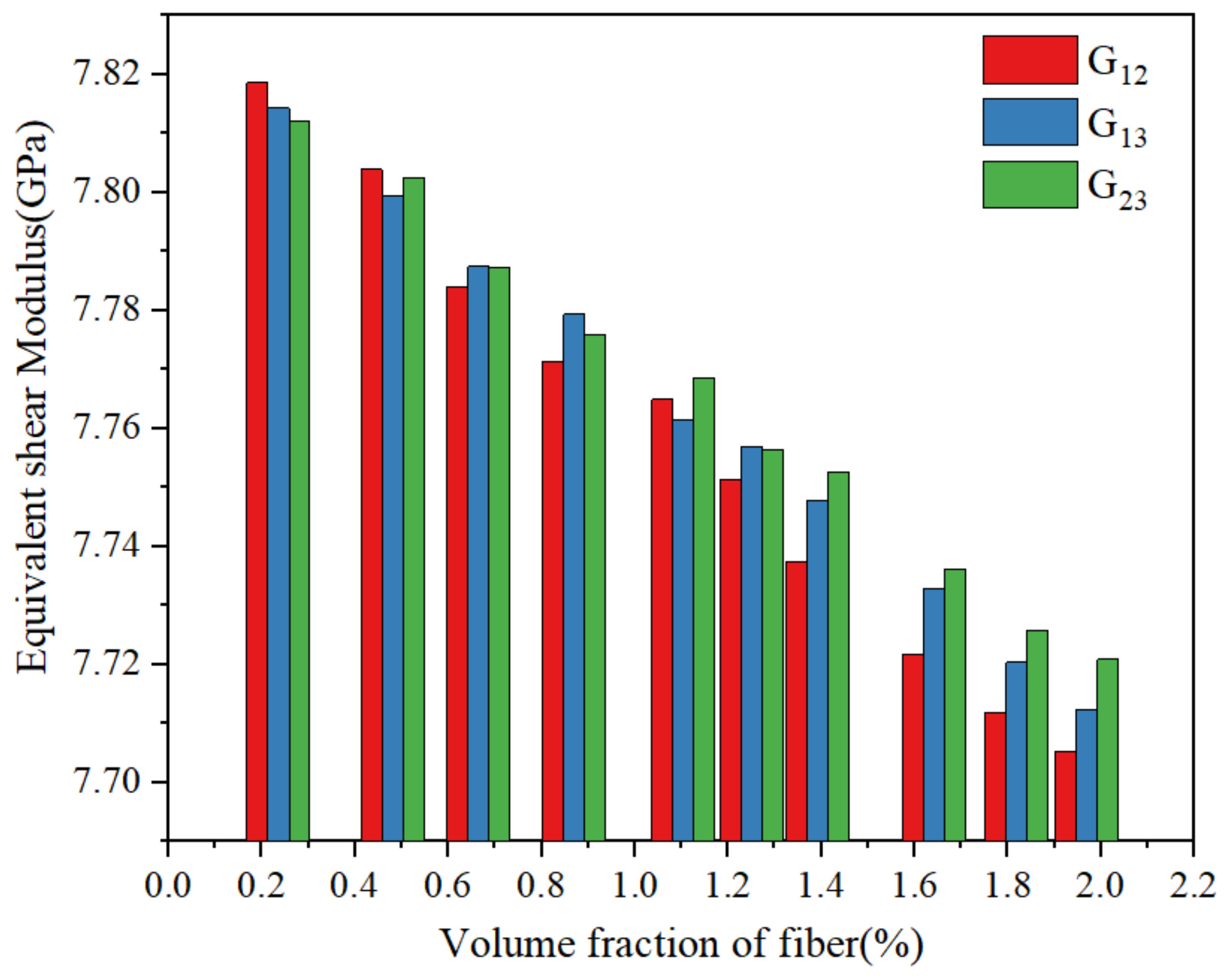
| (GPa) | 7.819 | 7.804 | 7.784 | 7.771 | 7.765 | 7.751 | 7.737 | 7.722 | 7.712 | 7.705 |
| (GPa) | 7.814 | 7.799 | 7.787 | 7.779 | 7.761 | 7.757 | 7.748 | 7.733 | 7.720 | 7.712 |
| (GPa) | 7.812 | 7.803 | 7.787 | 7.776 | 7.769 | 7.756 | 7.753 | 7.736 | 7.726 | 7.721 |
| 0.277 | 0.277 | 0.276 | 0.276 | 0.275 | 0.275 | 0.274 | 0.274 | 0.274 | 0.273 | |
| 0.278 | 0.277 | 0.277 | 0.276 | 0.276 | 0.275 | 0.274 | 0.274 | 0.274 | 0.273 | |
| 0.277 | 0.276 | 0.276 | 0.276 | 0.276 | 0.275 | 0.275 | 0.274 | 0.273 | 0.273 |
Publisher’s Note: MDPI stays neutral with regard to jurisdictional claims in published maps and institutional affiliations. |
© 2022 by the authors. Licensee MDPI, Basel, Switzerland. This article is an open access article distributed under the terms and conditions of the Creative Commons Attribution (CC BY) license (https://creativecommons.org/licenses/by/4.0/).
Share and Cite
Long, X.; Su, T.; Chen, Z.; Su, Y.; Siow, K.S. Tunable Coefficient of Thermal Expansion of Composite Materials for Thin-Film Coatings. Coatings 2022, 12, 836. https://doi.org/10.3390/coatings12060836
Long X, Su T, Chen Z, Su Y, Siow KS. Tunable Coefficient of Thermal Expansion of Composite Materials for Thin-Film Coatings. Coatings. 2022; 12(6):836. https://doi.org/10.3390/coatings12060836
Chicago/Turabian StyleLong, Xu, Tianxiong Su, Zubin Chen, Yutai Su, and Kim S. Siow. 2022. "Tunable Coefficient of Thermal Expansion of Composite Materials for Thin-Film Coatings" Coatings 12, no. 6: 836. https://doi.org/10.3390/coatings12060836
APA StyleLong, X., Su, T., Chen, Z., Su, Y., & Siow, K. S. (2022). Tunable Coefficient of Thermal Expansion of Composite Materials for Thin-Film Coatings. Coatings, 12(6), 836. https://doi.org/10.3390/coatings12060836