An Experimental Analysis of Microcrack Generation during Hydraulic Fracturing of Shale

Abstract

Hydraulic fracturing is commonly applied in the shale gas exploitation industry. However, the mechanical mechanism of permeability under fracturing has so far been unclear. In this study, an analysis of laboratory experiments on hydraulic fracture propagation and bedding plane reactivation in shale is presented. To investigate microcrack occurrence under fracturing, several small slices were collected from the fracture surface and scanned with a scanning electron microscope (SEM). It was found that observed microscopic microcracks could not be produced by fluid pressure as the latter generated compressive stresses at the site of microcracks. Rather, the microcracks were produced by tensile stress concentration in front of the propagating fracture. This implies that bedding plane reactivation was caused by fracture propagation along the plane. An analysis of microcrack lengths showed that shale exhibited anisotropy in fracture toughness with resistance to fracture propagation parallel to bedding planes being twice as small compared to resistance to fracture propagation in the direction normal to bedding planes.

1. Introduction

The complex pore structure of shale can provide storage spaces for shale gas [1,2]. The fracture network generated by hydraulic fracturing is intended to form a dense hydraulically conductive pathway connecting as many isolated hydrocarbon-rich pores as possible to increase permeability. Hydraulic fracture tends to be a dominating fracture in the network with random multiple branches (secondary fractures). When a hydraulic fracture is induced near an injection port that is maintained at a relatively high injection pressure, a secondary fracture can grow at a markedly lower fluid pressure than that of the main fracture [3,4]. In addition, in previous studies [5,6,7], some microcracks have been observed near the hydraulic fractures or on the fracture surfaces. While considerable efforts have been directed towards modeling hydraulic fracturing [8,9,10], the role of microcracks that are induced as a result of hydraulic fracturing cannot be ignored. It is usually assumed that fracturing fluids with low viscosity, such as water or CO₂, tend to induce widely extending fractures with many microcrack branches [11,12]. The densely distributed microcracks around the main fracture can increase shale permeability by connecting pores with macrofractures [13]. More importantly, the process of microcrack generation at the fracture surface is detectible and can shed light on the mechanism of fracture propagation.

The degree of microcracking can vary depending on the fracturing fluid, rock type, stress or temperature boundary conditions, as well as inherent material properties and heterogeneities [14]. Stanchits et al. [15] studied the effects of fluid viscosity and injection rate on the hydraulic fracture propagation in heterogeneous rock. Fracturing with high-viscosity fluids resulted in stable fracture propagation initiated before breakdown, while fracturing with low-viscosity fluids resulted in unstable fracture propagation initiated almost simultaneously with breakdown. When using high-viscosity fluids at high rates, fracture initiation occurred prior to breakdown. We note, however, that these features are a consequence of the viscosity-controlled interaction between the pressure created by the fracturing fluid, fracture opening and the hydrodynamics of fluid flow [16,17] rather than an effect of microcracking and its mechanisms.

The orientation of the induced fracture agrees with the applied stress direction in isotropic materials, while in anisotropic materials, the fracture direction depends on the direction and magnitude of stress applied with respect to the foliation and the magnitude of anisotropy. For example, Chitrala et al. [18] and Kumari et al. [19] performed a series of hydraulic fracturing experiments on granite under a wide range of confining pressures and temperatures. The results showed that the heterogeneity of the rock matrix can result in complex fracture patterns exhibiting multiple fractures along weaker planes of the matrix. Due to the injection of cold fluid into the rock fractures, the propagation of multiple microcracks can be triggered, mainly close to the wellbore.

Throughout the hydraulic fracturing process, stress concentrations are induced in the rock mass which can cause microcracking within the bulk material and along the pre-existing discontinuities, grain boundaries and bedding planes. Hampton et al. [14], using techniques of remote microcrack detection mostly based on acoustic or microseismic emission, observed that the process of microcrack generation can be utilized for hydraulic fracture growth monitoring and can provide the information needed to avoid fracking-related environmental damage. Maxwell et al. [20] used microseismic monitoring to image hydraulic fracture growth in the Barnett Shale. The microseismic images illustrated the fracture geometry and complexity for the first time in the field of large-scale hydraulic fracturing.

Some researchers have used acoustic or microseismic emission to better understand the source mechanism of microcracking, in particular to determine whether the microcracks are tensile, shear, or mixed mode (tensile or shear). Ishida [21] suggested that the rock grain size affects the source mechanism of microcrack generation. Fault plane solutions of acoustic emission (AE) indicated that shear fracturing was dominant in specimens having larger grains, whereas tensile fracturing was dominant in those having smaller grains. There was also some minor shearing along the grain boundaries between segments of tensile cracks. Stoeckhert et al. [22] concluded that fracking-induced microcracks were mostly tensile, given the internal pressurization of the flaws. In addition, many scholars, including Ishida et al. [23], Gonçalves and Einstein [24], Hampton et al. [25], and Li et al. [26] have retrieved microcrack locations and identified development stages based on interpretation of AE signals during hydraulic fracturing. Most of the AE studies were successful in characterizing the microcrack locations and distributions but had limited success in interpreting microcrack formation mechanisms during hydraulic fracturing.

In the present paper, in Section 2, microcracking observed in laboratory experiments through scanning electron microscope (SEM) images of hydraulic fracturing and bedding plane reactivation in shale are analyzed. Section 3 presents possible mechanisms of microcrack generation under the conditions of the fracturing experiments. Following the abovementioned analyses, in Section 4, the notion of anisotropy of fracture toughness is developed, based on the hydraulic fracturing experiments.

2. Microcracks Generated along the Fractures

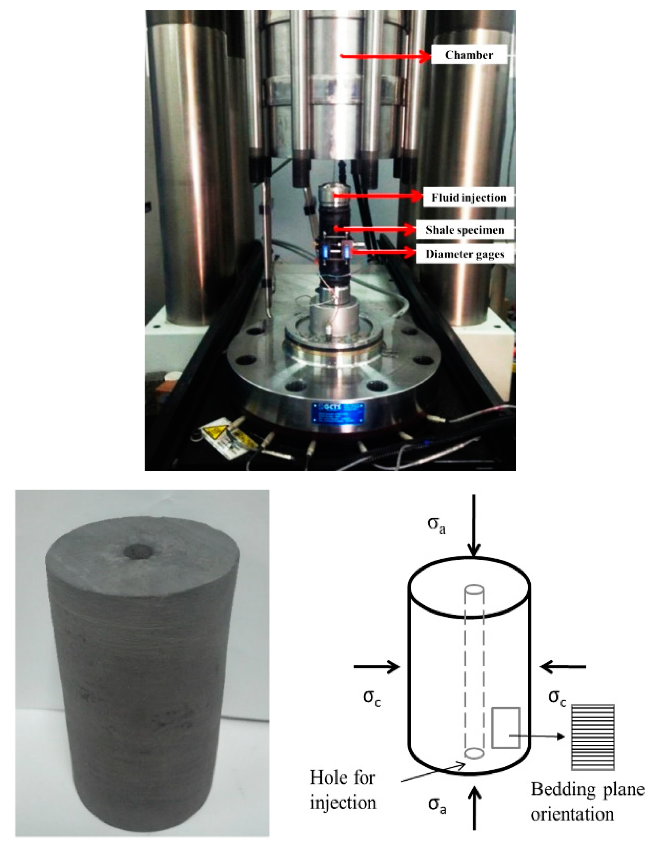
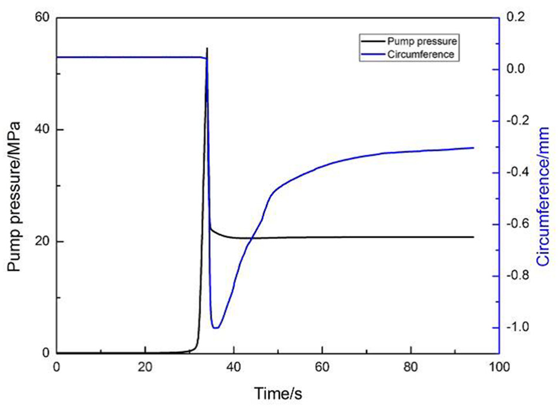
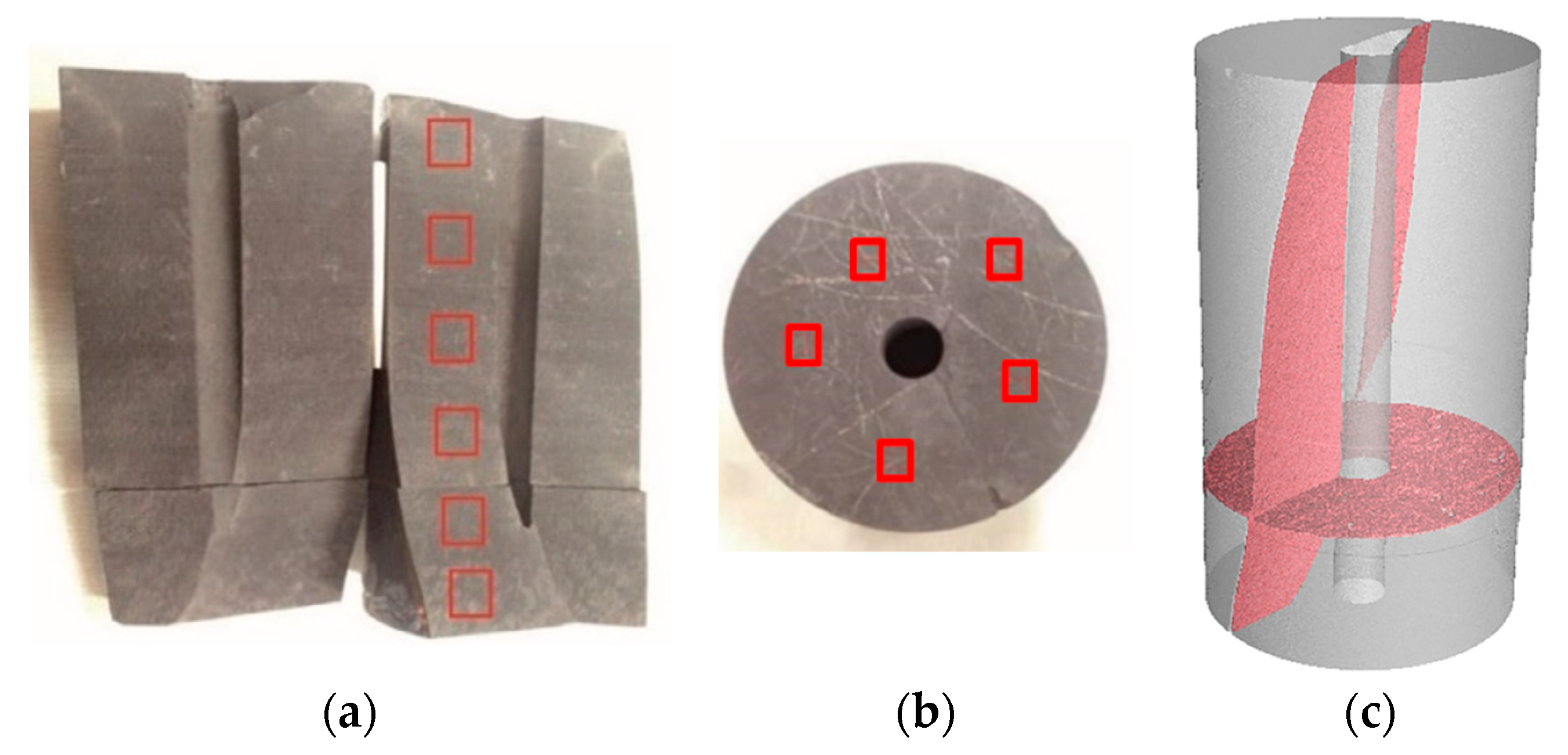
2.1. Shale Fracturing in the Experiment

Hydraulic fracturing experiments were performed on the shale specimens cored from the Silurian Longmaxi shale formation in southern Sichuan Basin of China, which is well known for its abundant shale gas reserves. The specimens were 50 mm in diameter and 100 mm in height and cylindrical in shape. A borehole of 8 mm diameter was drilled at the center along the cylinder axis to produce hydraulic fracture (Figure 1). The hydraulic fracturing experiments were carried out on the GCTS RTX-3000 triaxial rock testing system (manufacturer: GCTS, Beijing, China) which allows for triaxial loading of rock specimens with simultaneous injection of fracturing fluid. Triaxial loadings of 25 MPa in axial stress and 20 MPa in confining stress were first applied to the specimens to simulate geostress conditions. Then fracturing of the shale specimens was conducted by injection of water into the central borehole. The injection rate of the fracturing fluid was set as 0.3 mL/s. Figure 2 shows typical pump pressure and circumference deformation development during the fracturing process. The pump pressure of the water injection increased drastically to a peak value of 54.56 MPa until the occurrence of breakdown. Simultaneously, the circumference of the shale specimen also increased sharply to a peak value of 1.0 mm. After fracturing, the shale specimen was retrieved from the pressure chamber for further observation. Each specimen showed a newly produced fracture (PF) along the axial direction and a reactivated fracture (RF) along the existing bedding plane in the fracturing experiment.

To investigate the microcracks on the fracture face, small slices were collected from the fracture faces. Six slices with dimensions of 5 mm × 5 mm were obtained from the newly produced fracture and five slices with dimensions of 3 mm × 3 mm were obtained from the reactivated fracture along the bedding plane, as shown in Figure 3. All the shale slices were polished by argon-ion to create a smooth surface for enhanced SEM images. The slices were imaged through a Zeiss Crossbeam (Carl Zeiss AG, Jena, Germany) 540 scanning microscope equipped with 4Q-ESD (energy dispersive spectroscopy). For better clarity of imaging, an acceleration voltage of 15 kV, with a working distance of approximately 8–10 mm, was used for the quantitative and qualitative identification of minerals by energy dispersive spectroscopy (EDS). An FIB-SEM system (Crossbeam 550, Carl Zeiss AG, Beijing, China) was also equipped in the laboratory for nanofabrication and serial cross-sectional imaging, which could be used to create 3D image stacks for the microcracks along the fracture face.

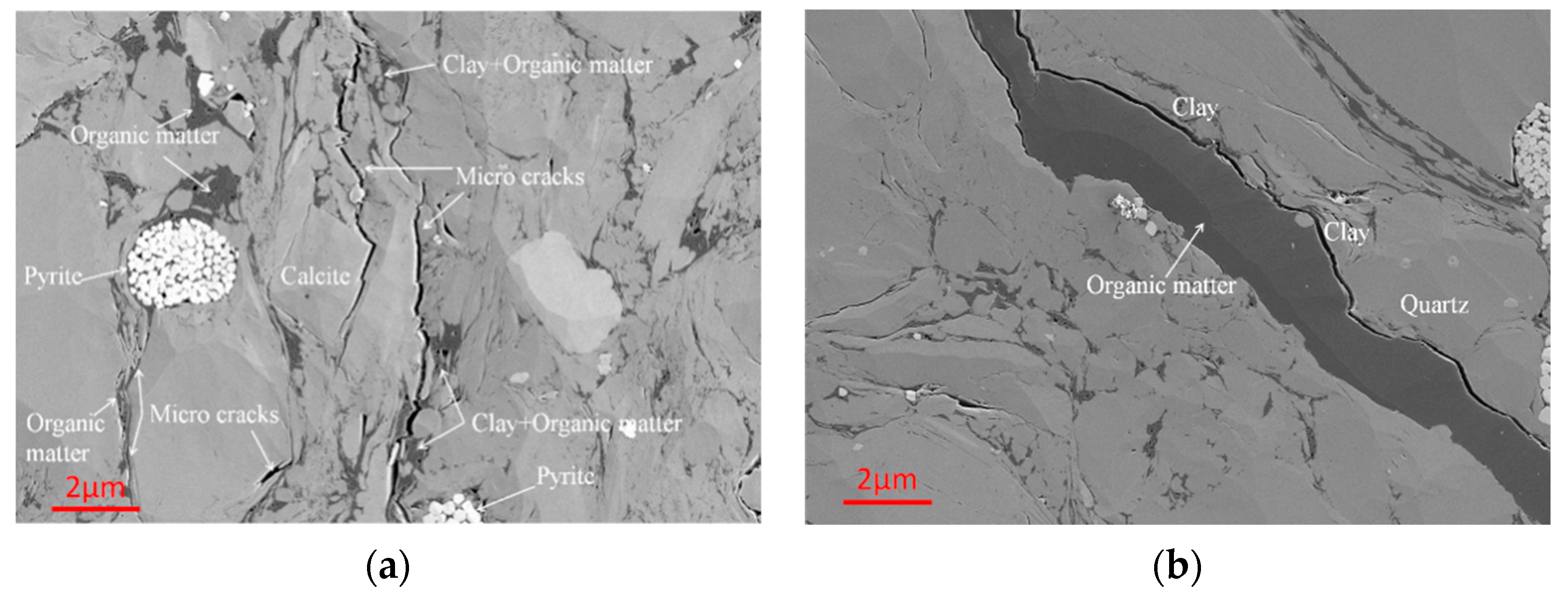
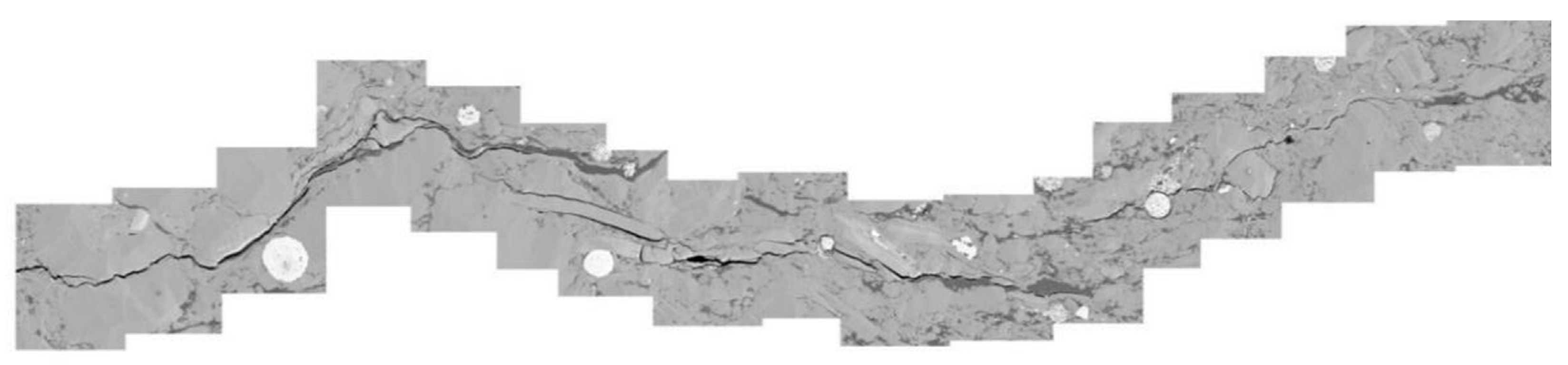
2.2. Microcrack Traces

Figure 4 shows typical SEM images of microcracks. The microcracks typically developed along the boundaries of the different mineral grains and organic matter. The tortuous microcracks showed various values of width, ranging from several nanometers to around 200 nm [6]. In addition, branching occurred along the pathways of these microcracks, which increased the complexity of the microcracks and provided more channels for gas release in nanopores. The parameters microcrack length and branching were used for the characterization of microcracks.

Quantitative description of the microcracks along the fractures depended on the characterization of length and distribution. To accomplish this, a total of 1195 SEM images were spliced into 34 larger images. The microcracks could be observed clearly and used for investigation. Figure 5 shows a spliced image illustrating the profile of microcracks induced by hydraulic fracturing. The generation of microcracks was complicated due to the presence of minerals, organic matter and pores along the pathway. The microcracks on newly produced fractures were generally oriented along the maximum principal stress axis, while microcracks on the reactivated microcracks were oriented randomly.

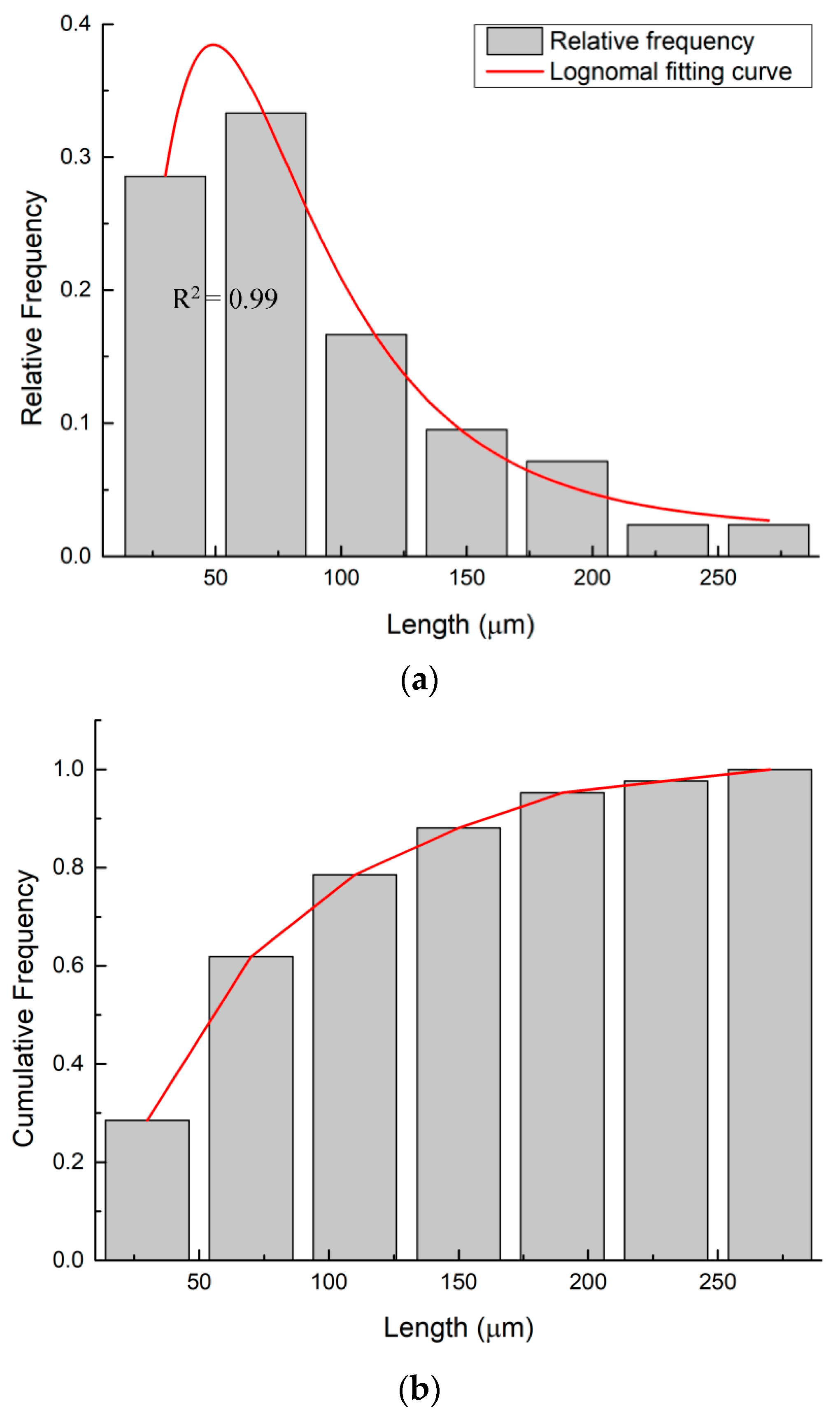
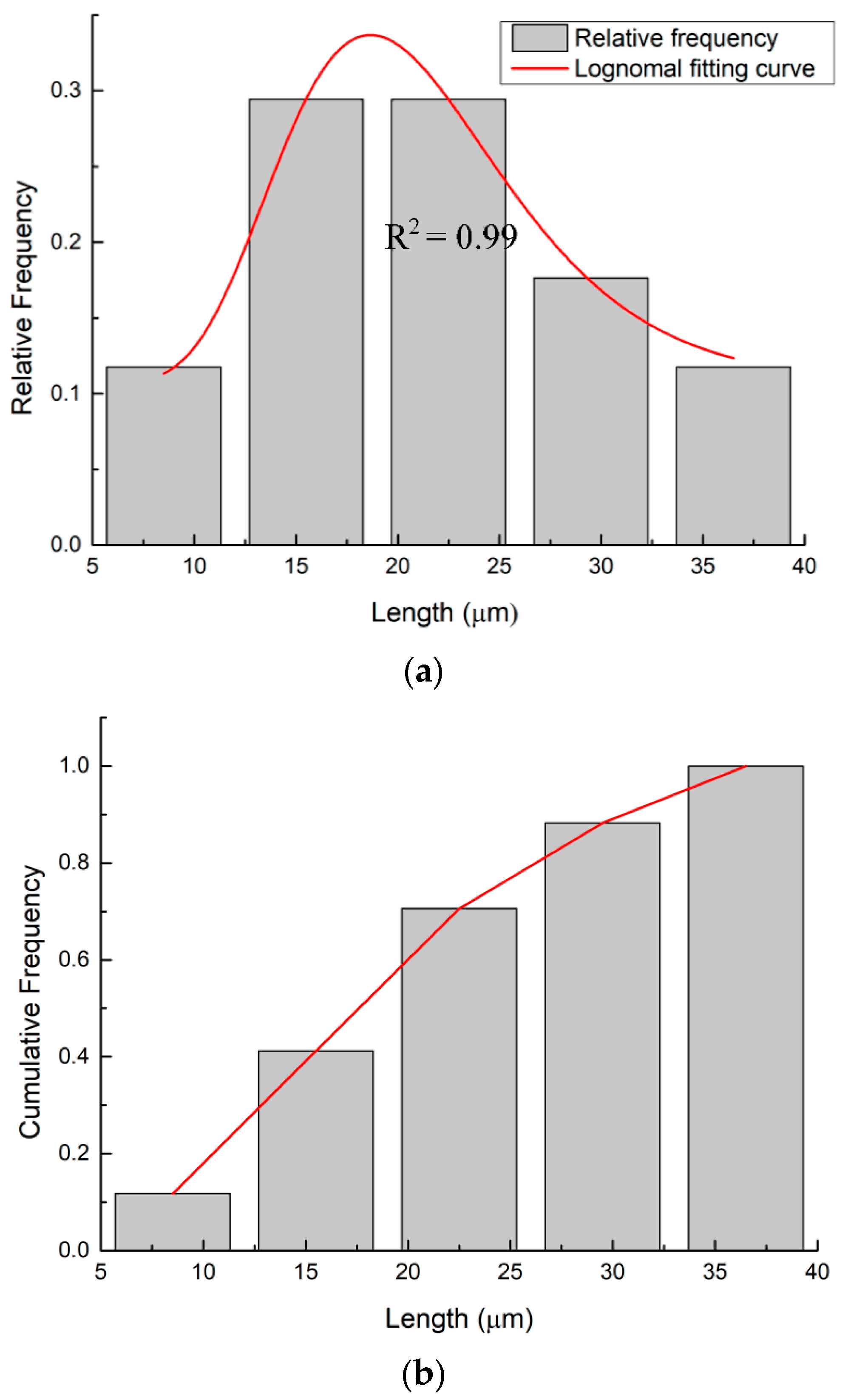
2.3. Distribution of Microcrack Lengths

Table 1. Mean value and standard deviation of the length of the microcracks.

Microcrack Pattern	Average Value (µm)	Standard Deviation (µm)
Newly PF	92.62	57.49
RF	21.55	7.83

summarizes the average length and standard deviation of the distribution of microcracks observed along the newly produced fracture and reactivated fracture. The average length of the microcracks along the newly produced fracture was 92.62 µm with a standard deviation of 57.49 µm. The average length of microcracks along the reactivated fracture was 21.55 µm with a standard deviation of 7.83 µm. An obvious gap was evident between the different microcrack patterns on the newly produced fracture and the reactivated fracture.

The frequency distribution histograms of the microcracks along the newly produced fracture and the reactivated fracture are shown in Figure 6 and Figure 7, respectively. The lognormal fitting curves were generally consistent with the microcrack length distribution. The lognormal probability density function of the microcrack lengths is:

$$f\left(x\right)=\frac{1}{x}\times \frac{1}{\Delta \sqrt{2\pi }}\exp \left(-\frac{{\left(\ln x-\delta \right)}^2}{2{\Delta }^2}\right)$$

(1)

where δ and ∆ are the mean and standard deviation of the logarithm of the microcrack length, respectively.

Table 2. Parameters of fitted lognormal distributions of the microcrack lengths.

Microcrack Pattern	δ	$\mathbf{\Delta }$	${\mathit{e}}_{\mathit{f}}$	${\mathit{s}}_{\mathit{f}}$
Newly PF	4.34	0.63	93.69	65.71
RF	3.00	0.40	21.76	9.06

summarizes the parameters of the fitted lognormal distributions for the microcracks generated along the new PF and RF, in which $e_f$ and $s_f$ are the average and standard deviation of the microcrack length determined by the fitted lognormal data, respectively.

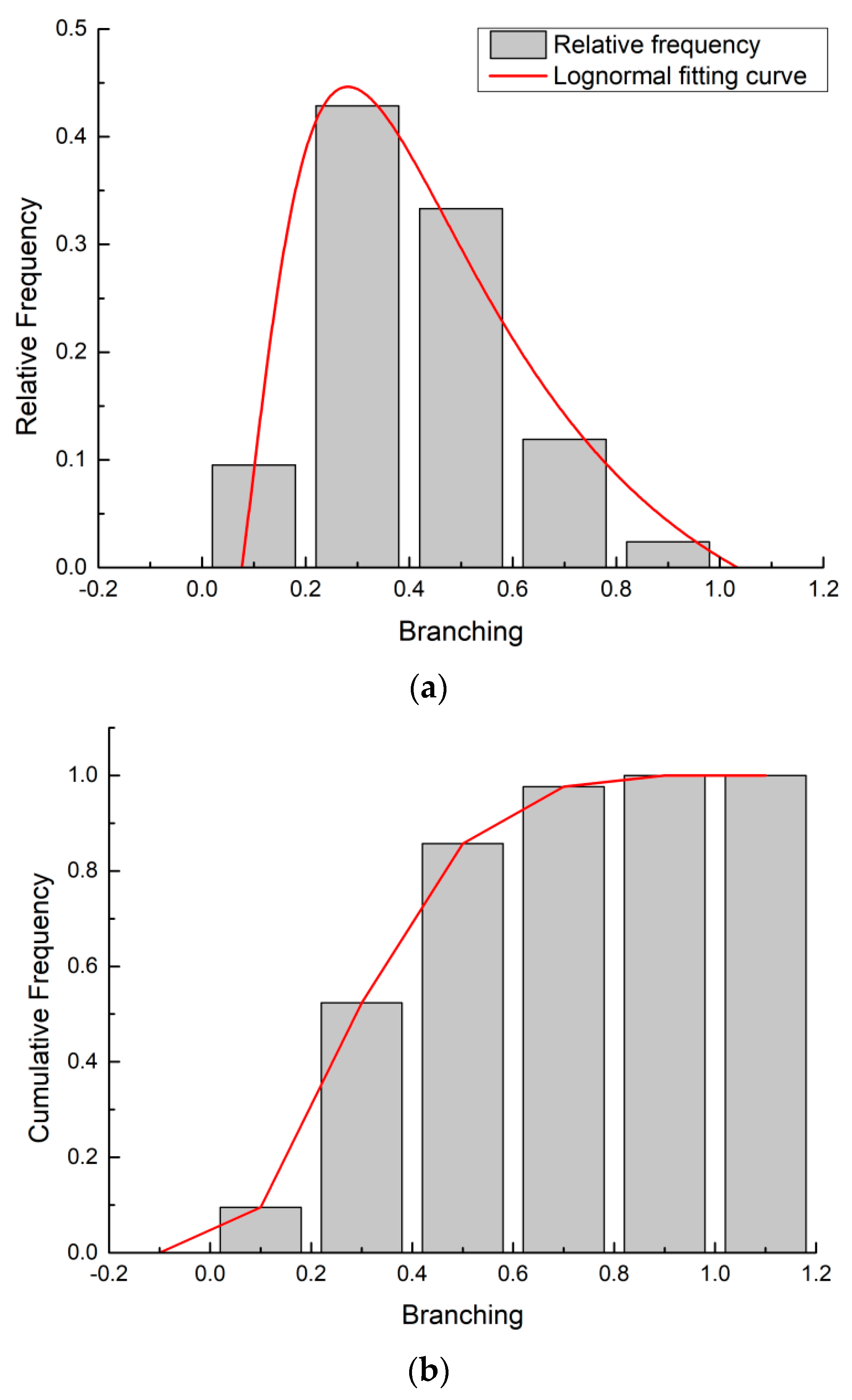
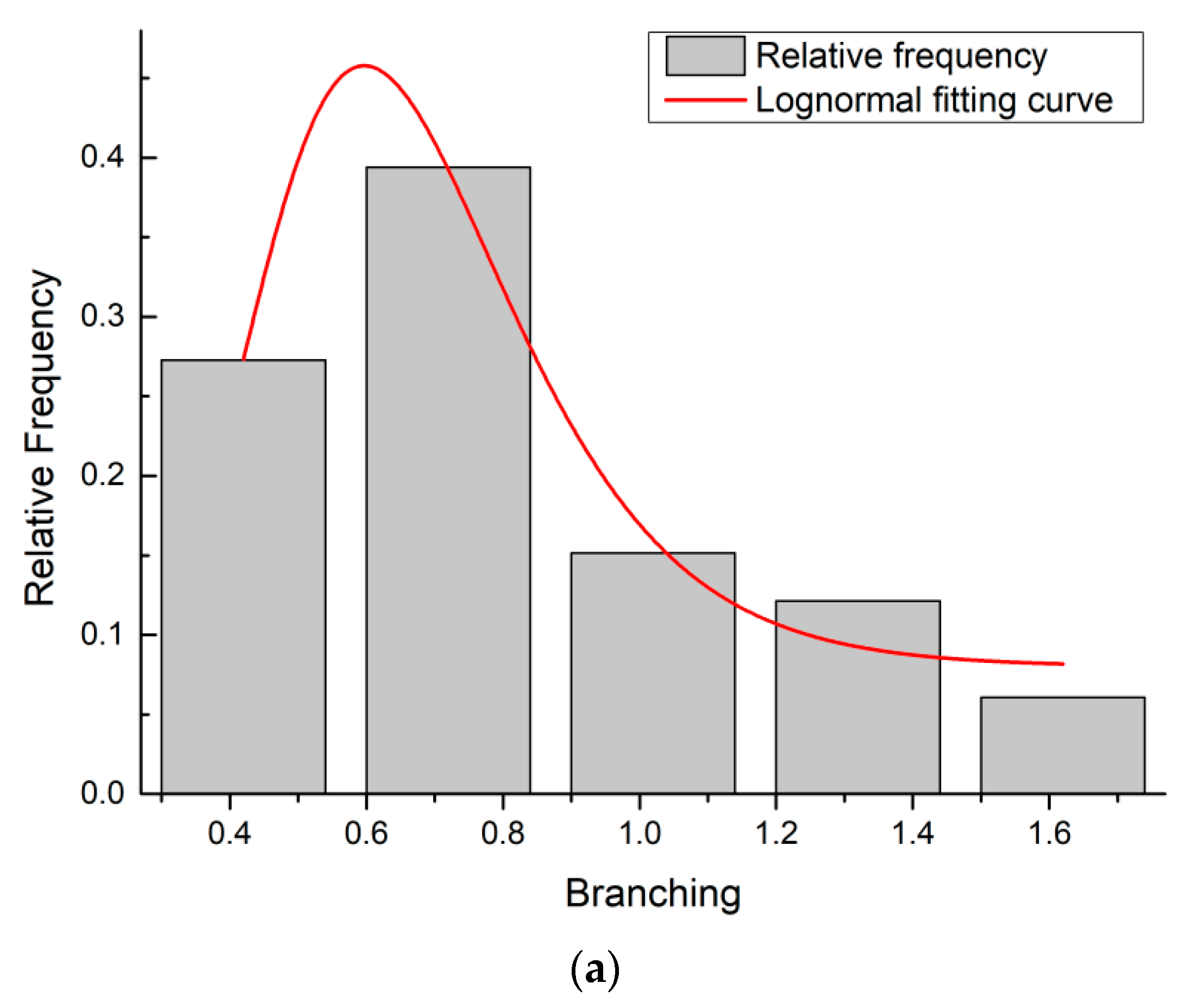
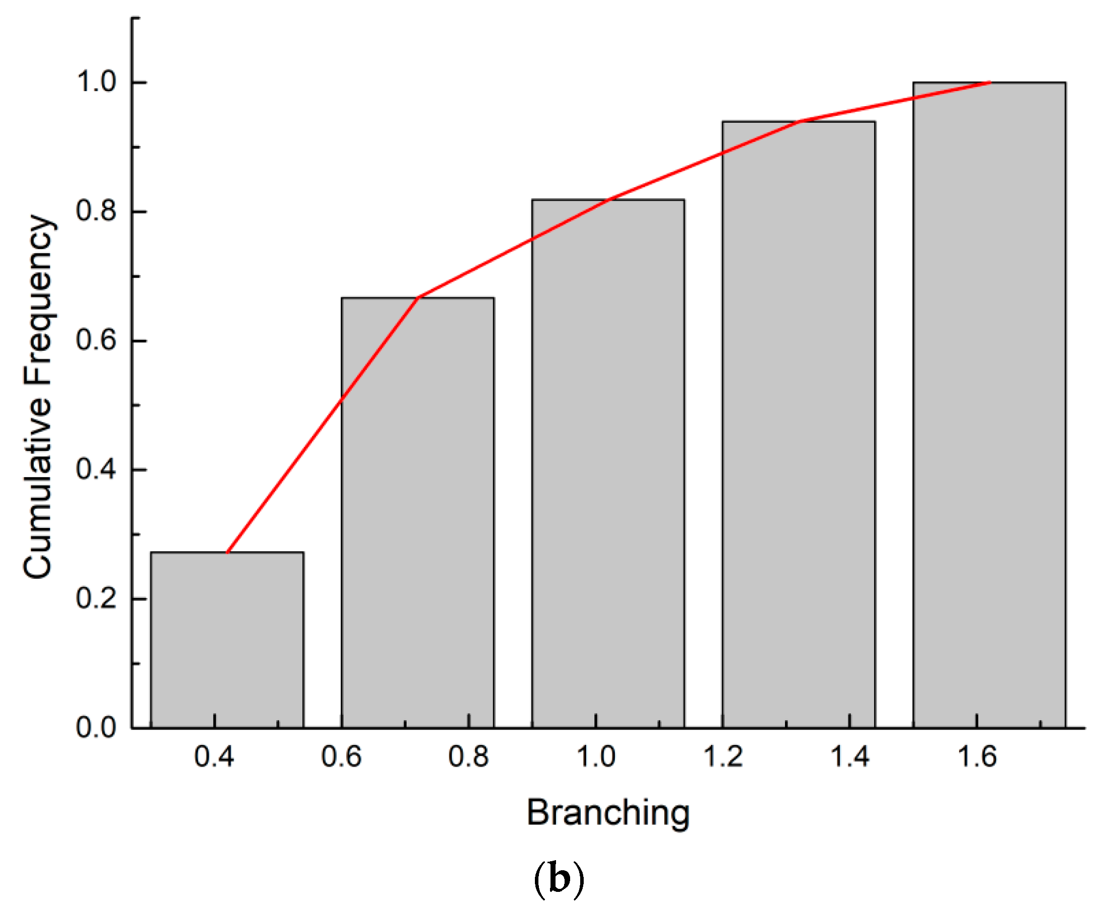
2.4. Distribution of the Branching Numbers

Based on the SEM observation results, branching of the microcracks was also investigated. Branching here refers to the branching number of a microcrack along the microcrack pathway per 10 µm.

Table 3. Average value and standard deviation of microcrack branching.

Microcrack Pattern	Average Value (µm)	Standard Deviation (µm)
newly PF	0.39	0.17
RF	0.87	0.38

summarizes the mean branch values and standard deviations of the data represented in Figure 8 and Figure 9. The average branching value of the measured microcracks on the newly produced fracture was 0.39 with a standard deviation of 0.17. The average branching value of the measured microcracks on the reactivated fracture was 0.87 with a standard deviation of 0.38.

3. Mechanics of Microcrack Formation at the Fracture Face

3.1. Possibility of Microcrack Formation by the Fracturing Fluid

The observations presented in the previous section show multitudes of microcracks generated along the fracture faces. It is often assumed that the microcracks at the fracture face are developed by the pressure of the fracturing fluid in hydraulic fracturing. To check this assertion, a simplified model of hydraulic fracture as a disc-like fracture of radius R, in rock modeled as isotropic elastic material, as shown in Figure 10, is considered. In Figure 10, $\rho \le R$ is a coordinate of a point on the fracture face, $\left(n, \tau , z\right)$ are local coordinates at point A of the fracture contour, and r is the radius vector to the point of the rock in the vicinity of fracture contour. The fracture is considered to be opened by uniform normal pressure p applied to fracture faces from inside which models the action of the fracturing fluid.

To determine if the fracturing fluid pressure could create microcracks at the fracture face, we used the elastic solution for the stress field around a disc-like crack (e.g., Kachanov, et al., 2003). For a point on a crack face ($z=0$), distanced from the center at $\rho \le R$ (due to the cylindrical symmetry the stress depends only on the distance from the center), the stress components read (compressive stress is positive)

$$\{\begin{array}{c}{\sigma }_x+{\sigma }_y=\frac{2p}{\pi }\left(1+2\nu \right)\left[\frac{R\sqrt{l_2^2-R^2}}{l_2^2-l_1^2}-\arcsin \frac{R}{l_2}\right]\\ {\sigma }_x-{\sigma }_y+2i{\sigma }_{xy}=\frac{2p}{\pi }\left(1-2\nu \right)\frac{R{l}_1^2\sqrt{l_2^2-R^2}}{l_2^2\left(l_2^2-l_1^2\right)}\\ {\sigma }_{xy}+i{\sigma }_{yz}=0,\hspace{1em}{\sigma }_z=p\end{array}$$

(2)

where $\nu$ is Poisson’s ratio and for $\rho \le R$, $l_1=\rho , l_2=R$. From here the stress components at the fracture face are

$${\sigma }_x={\sigma }_y=\left(\nu +\frac{1}{2}\right)p,\hspace{1em}{\sigma }_z=p,\hspace{1em}{\sigma }_{xy}={\sigma }_{yz}=0$$

(3)

It is seen that rock at the fracture faces is under triaxial compression with

$$\frac{1}{2}\le {\sigma }_x={\sigma }_y\le {\sigma }_z=p,\hspace{1em}{\sigma }_{xy}={\sigma }_{yz}=0$$

(4)

This excludes the formation or propagation of tensile microcracks at the fracture face, since the triaxial compressive strength is much higher compared to the rock tensile strength. Furthermore, even driving pre-existing microcracks by penetrating fracturing fluid does not seem to be possible as the excess of the fluid pressure over ${\sigma }_x={\sigma }_y$ is $p-{\sigma }_x=\left(1/2-\nu \right)p\le 1/2p$. Therefore, the excess of the fluid pressure is smaller than half of the pressure needed to drive the hydraulic fracture. In other words, this fluid pressure would be insufficient to drive even large fractures to say nothing of much smaller pre-existing tensile microcracks (the smaller the cracks, the larger the stress needed to initiate their propagation). This is at variance with what is usually assumed in the literature [22].

Consider now the possibility of reactivating pre-existing microcracks as shear (Mode II or III) cracks. Assume that the pre-existing microcracks are randomly oriented. Then, the conditions of sliding over a suitable oriented microcrack whose faces are prevented from sliding by friction are determined by the conventional Mohr–Coulomb criterion [27]. According to this criterion microcrack reactivation will occur when the two stress components ${\sigma }_x={\sigma }_y$, ${\sigma }_z$ satisfy the following relationship

$${\sigma }_z=\frac{2c \cos \phi +{\sigma }_x\left(1+\sin \phi \right)}{\left(1-\sin \phi \right)}$$

(5)

where $c$ and $\phi$ are cohesion and friction angle respectively. Assuming $c=0$ (this is the most favorable case for microcrack reactivation), and substituting stress components (3) into Equation (5), one obtains the maximum value of friction angle, ${\phi }_{max}$, that allows microcrack reactivation:

$$\sin {\phi }_{max}=\frac{1-2\nu }{3+2\nu }$$

(6)

The highest value of ${\phi }_{max}=19.5°$ corresponds to $\nu =0$, while, for a typical value of Poisson’s ratio of $\nu =0.25$, the friction angle allowing the microcrack formation is even smaller: ${\phi }_{max}=8.2$. Therefore, the friction angles allowing shear microcrack formation need to be quite small even in the absence of cohesion.

It is seen that, for the pre-existing microcracks to be reactivated, the friction angle and the Poisson’s ratio should be low. While it is not impossible, microcrack reactivation is a regular occurrence, therefore a more robust mechanism, independent of the rock properties, should be at work. Such a mechanism is considered in the following subsection.

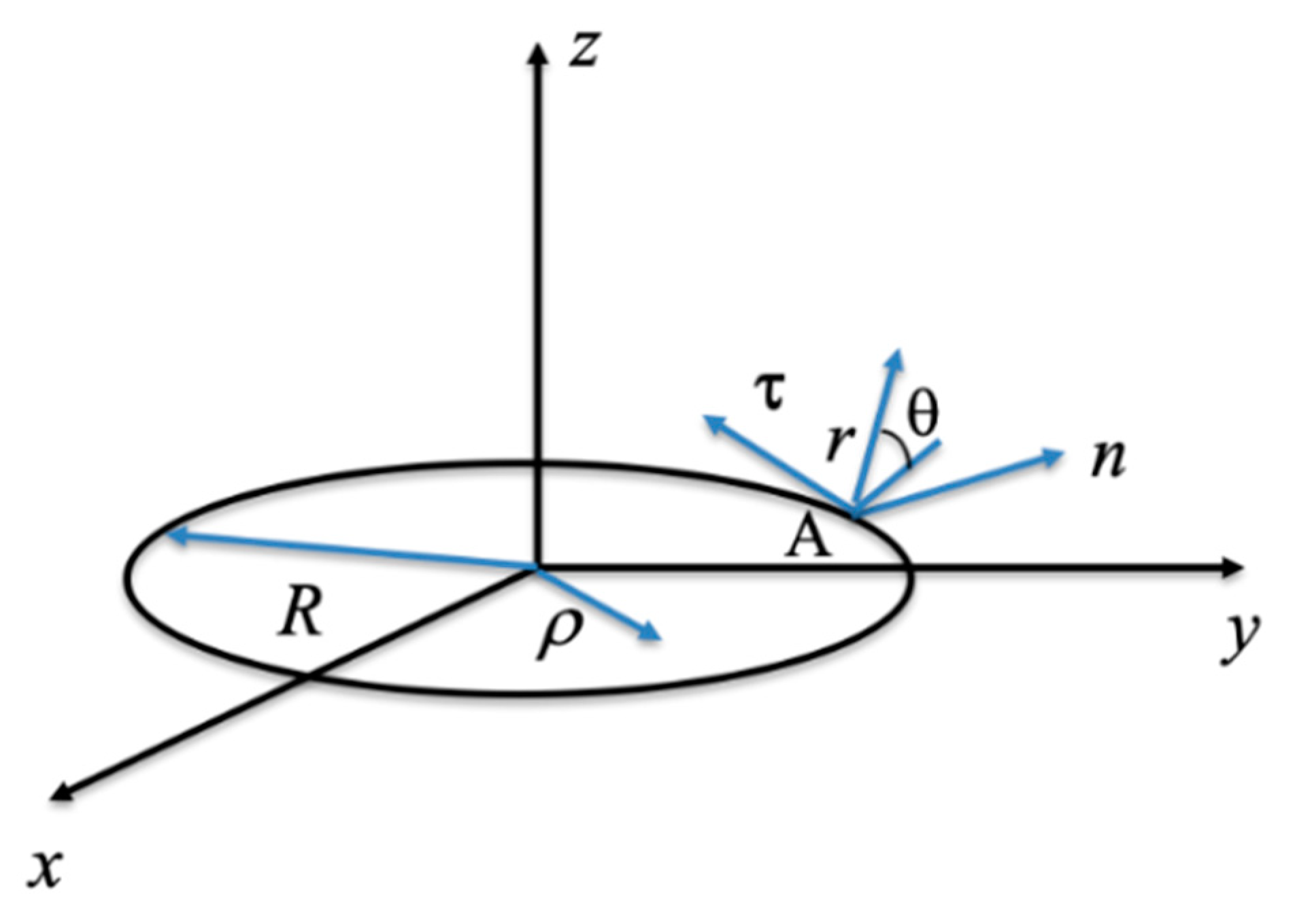
3.2. Microcrack Formation in the Process of Hydraulic Fracture Growth by Singular Stresses at Its Contour

To analyze the stress singularity mechanism of microcrack formation, we consider a point A at the contour of the disc-like fracture that models the hydraulic fracture, as shown in Figure 10. The components of stress singularity at this point have, in the co-ordinate frame (n, τ, z), the following form [28]; it is assumed that tensile stresses are negative:

$$\{\begin{array}{c}{\sigma }_n=-\frac{K_I}{4\sqrt{2\pi r}}\left(3\cos \frac{\theta }{2}+\cos \frac{5\theta }{2}\right)\\ {\sigma }_{\tau }=-\frac{2\nu K_I}{\sqrt{2\pi r}}cos\frac{\theta }{2}\\ {\sigma }_z=-\frac{K_I}{4\sqrt{2\pi r}}\left(5\cos \frac{\theta }{2}-\cos \frac{5\theta }{2}\right) \end{array}$$

(7)

where

$$K_I=2p\sqrt{R/\pi }$$

(8)

is the Mode I stress intensity factor developed by a disc-like crack under internal pressure p. Here we only consider the singular terms in the expression for the stress filed at the fracture contour that neglects the non-singular terms, in particular, the compressive stress field created by the compressive loading.

Obviously, the components of stress (7) assume maximum values when $\theta =0$. The tensile stress components (negative) acting on the planes normal to the fracture face, which are the stresses capable of producing microcracks (or driving the pre-existing ones), are

$${\sigma }_{n,max}=-\frac{K_I}{\sqrt{2\pi r}},\hspace{1em}{\sigma }_{\tau ,max}=2\nu {\sigma }_{n,max}<{\sigma }_{n,max}$$

(9)

From here it is clear that the microcracks normal to the fracture face can be generated by the stress component ${\sigma }_{n,max}$. They are formed ahead of the fracture (in front of the fracture contour, ρ > R) in the direction normal to the direction of the fracture propagation. Since the fracture propagates in all directions in its plane, the new (developed) microcracks can, in principle, assume all orientations unless they are directed by the externally applied compressive stress. The effect of the externally applied compressive stress is based on the fact that while formally stresses (9) tend to infinity as r → 0, in reality there exists a characteristic length d associated with the rock microstructure such that stresses (8) refer to distances r ≥ d. Therefore, these stresses become non-singular or finite [29]. Therefore, the magnitudes of these stresses can become comparable to the magnitude of the externally applied stress (compression in the experiments described in Section 2), and hence the external compressive stress can dictate the directions at which the microcracks can be formed.

The above analysis suggests that: (1) Microcracks formed by the stress singularity ahead of the hydraulic fracture are caused by the fracturing fluid pressure inside the fracture rather than by the pressure of fluid itself; (2) The microcracks are mostly tensile, formed by the tensile stresses ${\sigma }_{n,max}$ created ahead of the propagating fracture, or a fracture formed in the bedding plane (a pre-existing weak plane) as a result of its reactivation; (3) The microcracks are formed normal to the bedding plane (which is normal to the direction of applied compression) and are all oriented parallel to the direction of the applied compressive stress; (4) In the newly formed hydraulic fracture which propagates in the direction parallel to the direction of the maximum compressive principal stress, the microcracks mostly form parallel to the direction of compression.

4. Anisotropy in Fracture Toughness

While the mechanism of microcrack formation was found to be the same in both the newly PF and RF, the average length of microcracks (that is the average length of traces of microcracks) produced by the RF were about four times smaller than the average length of the microcracks produced by the new PF. Both the PF and RF were essentially Model I cracks. However, the fracture toughness, $K_{Ic}$, controlling their propagation, according to the classical fracture propagation criterion $K_I=K_{Ic}$, should be different in these two cases.

Let the local tensile stress of the rock which needs to be overcome to produce a microcrack be ${\sigma }_t$. This means that the microcrack gets formed when $\left|{\sigma }_{n,max}\right|={\sigma }_t$. It is reasonable to assume that ${\sigma }_t$ is the same for both new and reactivated fractures, since in both cases the microcracks appear outside the fractures, i.e., it is the intact rock that has to be fractured. Distance l at which the fracture-produced stress magnitude is equal to the local rock strength is controlled by the following criterion (in the approximation based only on the singular terms):

$${\sigma }_t=\frac{K_{Ic}}{\sqrt{2\pi l}}$$

(10)

When a microcrack is generated, it starts at a distance l from the fracture contour and then growth towards it as the stress increases with reduction in the distance from the contour. Let $l_f$ and $l_r$ be the average microcrack lengths for newly produced and reactivated fractures, respectively. Then Equation (10) suggests that the values of fracture toughness for the new and reactivated fractures should be different:

$$K_{Ic,f}={\sigma }_t\sqrt{2\pi l_f} ,\hspace{1em}{K}_{Ic,r}={\sigma }_t\sqrt{2\pi l_r}$$

(11)

Given the difference in the microcrack average lengths determined in Section 2 being $l_f/l_r=92.6/21.6=4.28$, the ratio of values of the fracture toughness is $K_{Ic,f}/K_{Ic,r}=2.1$. Thus, the fracture toughness for a new crack is two times higher than that for fracture reactivation.

There is, of course, a difference between the values of fracture toughness controlling Mode I crack propagation in the new fracture and in a bedding plane. Shale is a rock with many bedding planes, however, any attempt to drive a crack parallel to bedding planes will make it deviate causing it to grow in a bedding plane. Therefore, the fracture toughness in the direction parallel to the bedding planes is twice as small as the fracture toughness in a normal direction. We can regard this phenomenon as anisotropy in fracture toughness in shales, which needs to be taken into account when hydraulic fracture in the required direction is designed in.

5. Conclusions

The laboratory experiment in the present study demonstrated that the hydraulic fractures of shale, including two different types of newly produced fracture (PF) and reactivated fracture (RF), were tensile fractures driven by fluid pressure. The newly produced PF grew along the maximum principal stress, while the RF propagated along the pre-existing bedding plane. These fractures were accompanied by microcrack generation with an orientation normal to the fracture surface. Further analysis following the experiment showed that the microcracks were generated in the process of fracture propagation, not after hydraulic fracturing. Where fluid pressure created compressive stresses acting parallel to the fracture faces, microcracks were prevented—the only place where tensile stresses were generated was in front of the propagating fracture creating microcracks. Since microcracks were also formed at the surfaces of the RF, it is concluded that the process of reactivation corresponded to tensile fracture propagation as well.

The resistance to fracture propagation of the bedding plane was evidently smaller than that of the rock where the main hydraulic fracture propagated, which translated into the difference between the values of fracture toughness. The smaller fracture toughness of the bedding plane meant that the distances over which the tensile stress concentration generated microcracks were smaller than in other parts of the shale. This led to the traces of microcracks in the RFs being smaller than in a newly developed PF, which were the observed experiment results. It was also found that an approximately four times difference in the mean microcrack lengths translated into a two times difference in the values of fracture toughness. Given that a fracture propagating parallel to the bedding planes will deviate to propagate along the weak planes, the observed difference in the values of fracture toughness indicates a twofold fracture toughness anisotropy.

It is anticipated that the results obtained will assist in the modeling of hydraulic fracturing and forecasting of production capacity. Subsequent monitoring will be required for efficient hydrocarbon production and reduction in the environmental impacts of fracking operations.

References

1. Ross, D.; Mar, R. The importance of shale composition and pore structure upon gas storage potential of shale gas reservoirs. Mar. Petrol. Geol. 2009, 26, 916–927. [Google Scholar] [CrossRef]
2. Bernard, S.; Wirth, R.; Schreiber, A.; Schulz, H.; Horsfield, B. Formation of nanoporous pyrobitumen residues during maturation of the Barnett Shale (Fort Worth Basin). Int. J. Coal. Geol. 2021, 103, 3–11. [Google Scholar] [CrossRef]
3. Zhou, J.; Xue, C. Experimental Investigation of Fracture Interaction between Natural Fractures and Hydraulic Fracture in Naturally Fractured Reservoirs. In Proceedings of the 73rd European Association of Geoscientists and Engineers Conference and exhibition, Vienna, Austria, 23 May 2011. [Google Scholar]
4. Altammar, M.J.; Sharma, M.M.; Manchanda, R. The effect of pore pressure on hydraulic fracture growth: An experimental study. Rock Mech. Rock Eng. 2018, 51, 2709–2732. [Google Scholar] [CrossRef]
5. Guo, T.; Zhang, S.; Qu, Z.; Zhou, T.; Xiao, Y.; Gao, J. Experimental study of hydraulic fracturing for shale by stimulated reservoir volume. Fuel 2014, 128, 373–380. [Google Scholar] [CrossRef]
6. He, J.; Lin, C.; Li, X.; Zhang, Y.; Chen, Y. Initiation, propagation, closure and morphology of hydraulic fractures in sandstone cores. Fuel 2017, 208, 65–70. [Google Scholar] [CrossRef]
7. Zhao, Z.; Li, X.; He, J.; Mao, T.; Zheng, B.; Li, G. A laboratory investigation of fracture propagation induced by supercritical carbon dioxide fracturing in continental shale with interbeds. J. Petrol. Sci. Eng. 2018, 166, 739–746. [Google Scholar] [CrossRef]
8. Lecampion, B.; Bunger, A.; Zhang, X. Numerical methods for hydraulic fracture propagation: A review of recent trends. J. Nat. Gas Sci. Eng. 2017, 49, 66–83. [Google Scholar] [CrossRef] [Green Version]
9. Teufel, L.; Clark, J. Hydraulic Fracture Propagation in Layered Rock: Experimental Studies of Fracture Containment. SPE J. 1984, 24, 19–32. [Google Scholar] [CrossRef] [Green Version]
10. Tan, P.; Jin, Y.; Han, K.; Hou, B.; Chen, M.; Gu, X.; Gao, J. Analysis of hydraulic fracture initiation and vertical propagation behavior in laminated shale formation. Fuel 2017, 206, 482–493. [Google Scholar] [CrossRef]
11. Ishid, T.; Aoyagi, K.; Niwa, T.; Chen, Y.; Murata, S.; Chen, Q.; Nakayam, Y. Acoustic emission monitoring of hydraulic fracturing laboratory experiment with supercritical and liquid CO2. Geophys. Res. Lett. 2012, 39, 16309. [Google Scholar] [CrossRef] [Green Version]
12. Bennour, Z.; Ishida, T.; Nagaya, Y.; Chen, Y.; Nara, Y.; Chen, Q. Crack extension in hydraulic fracturing of shale cores using viscous oil, water, and liquid CO2. Rock Mech. Rock Eng. 2015, 48, 1463–1473. [Google Scholar] [CrossRef] [Green Version]
13. He, J.; Li, X.; Yin, C.; Zhang, Y.; Lin, C. Propagation and characterization of the micro cracks induced by hydraulic fracturing in shale. Energy 2020, 191, 116449. [Google Scholar] [CrossRef]
14. Hampton, J.; Gutierrez, M.; Matzar, L. Microcrack Damage Observations near Coalesced Fractures Using Acoustic Emission. Rock Mech. Rock Eng. 2019, 52, 3597–3608. [Google Scholar] [CrossRef]
15. Stanchits, S.; Burghardt, J.; Surdi, A. Hydraulic fracturing of heterogeneous rock monitored by acoustic emission. Rock Mech. Rock Eng. 2015, 48, 2513–2527. [Google Scholar] [CrossRef]
16. Garagash, D.; Detournay, E. The tip region of a fluid-driven fracture in an elastic medium. J. Mech. 2000, 67, 183–192. [Google Scholar] [CrossRef]
17. Bunger, A.P.; Detournay, E.; Jeffrey, R.G. Crack tip behavior in near-surface fluid-driven fracture experiments. Comptes Rendus Mécanique 2005, 333, 299–304. [Google Scholar] [CrossRef]
18. Chitrala, Y.; Moreno, C.; Sondergeld, C.H.; Rai, C. Microseismic and Microscopic Analysis of Laboratory Induced Hydraulic Fractures. In Proceedings of the Society of Petroleum engineers-Canadian Uncoventional Resources Conference, Calgary, AB, Canada, 17 November 2011. [Google Scholar]
19. Kumari, W.; Ranjith, P.; Perera, M.; Li, X.; Li, L.; Chen, B.; Isaka, B.; De Silva, V. Hydraulic fracturing under high temperature and pressure conditions with micro CT applications: Geothermal energy from hot dry rocks. Fuel 2018, 230, 138–154. [Google Scholar] [CrossRef]
20. Maxwell, S.C.; Urbancic, T.I.; Steinsberger, N.; Zinno, R. Microseismic Imaging of Hydraulic Fracture Complexity in the Barnett Shale. In Proceedings of the 2002 SPE Annual Technocal Coference and Exhibition, San Antonio, TX, USA, 29 September 2002. [Google Scholar]
21. Ishida, T. Acoustic emission monitoring of hydraulic fracturing in laboratory and field. Constr. Build. Mater. 2001, 15, 283–295. [Google Scholar] [CrossRef]
22. Stoeckhert, F.; Molenda, M.; Brenne, S.; Alber, M. Fracture propagation in sandstone and slate—Laboratory experiments, acoustic emissions and fracture mechanics. J. Rock Mech. Geotech. Eng. 2015, 7, 237–249. [Google Scholar] [CrossRef] [Green Version]
23. Ishida, T.; Chen, Q.; Mizuta, Y. Effect of injected water on hydraulic fracturing deduced from acoustic emission monitoring. Pure Appl. Geophys. 1997, 150, 627–646. [Google Scholar] [CrossRef]
24. Gonçalves, B.; Einstein, H. Physical processes involved in the laboratory hydraulic fracturing of granite: Visual observations and interpretation. Eng. Fract. Mech. 2018, 191, 125–142. [Google Scholar] [CrossRef]
25. Hampton, J.; Gutierrez, M.; Matzar, L.; H, D.; Frash, L. Acoustic emission characterization of microcracking in laboratory-scale hydraulic fracturing tests. J. Rock Mech. Geotech. Eng. 2018, 10, 805–817. [Google Scholar] [CrossRef]
26. Li, B.; Gonçalves, B.; Einstein, H. Laboratory hydraulic fracturing of granite: Acoustic emission observations and interpretation. Eng. Fract. Mech. 2019, 209, 200–220. [Google Scholar] [CrossRef]
27. Brady, B.H.G.; Brown, E.T. Rock Mechanics for Underground Mining; George Allen and Unwin: London, UK; Boston, MA, USA; Sydney, Australia, 1985. [Google Scholar]
28. Sih, G.C.; Liebowitz, H. Mathematical theories of brittle fracture. In Fracture, an Advanced Treatise; Liebowitz, H., Ed.; Mathematical Fundamentals; Academic Press: New York, NY, USA; London, UK, 1986; Volume II, pp. 68–191. [Google Scholar]
29. Dyskin, A.V. Crack growth criteria incorporating non-singular stresses: Size effect in apparent fracture toughness. Int. J. Fract. 1997, 83, 191–206. [Google Scholar] [CrossRef]
Figure 1. The experimental scheme and shale specimen.
Coatings 12 00483 g001
Figure 2. Pump pressure and circumference development during the fracturing process.
Coatings 12 00483 g002
Figure 3. Specimen after testing: (a) locations of the slices collected from the newly produced PF; (b) locations of the slices collected from the RF and (c) CT reconstruction of both hydraulic fractures in the shale specimen.
Coatings 12 00483 g003
Figure 4. Typical images of microcracks developing (a) along the boundaries of mineral grains and (b) organic matter.
Coatings 12 00483 g004
Figure 5. Spliced image (individual image size is 15 µm × 10 µm) showing microcracks.
Coatings 12 00483 g005
Figure 6. Length frequency histogram of the microcracks on the newly produced PF. (a) Relative frequency. (b) Cumulative frequency.
Coatings 12 00483 g006
Figure 7. Length frequency histogram of the microcracks on the RF. (a) Relative frequency. (b) Cumulative frequency.
Coatings 12 00483 g007
Figure 8. Branching frequency histogram of newly produced microcracks. (a) Relative frequency. (b) Cumulative frequency.
Coatings 12 00483 g008
Figure 9. Branching frequency histogram of reactivated microcracks. (a) Relative frequency. (b) Cumulative frequency.
Coatings 12 00483 g009aCoatings 12 00483 g009b
Figure 10. Model of hydraulic fracture as a disc-like crack of radius R.
Coatings 12 00483 g010