
Reconstruction Method of Old Well Logging Curves Based on BI-LSTM Model—Taking Feixianguan Formation in East Sichuan as an Example

Abstract
:1. Introduction
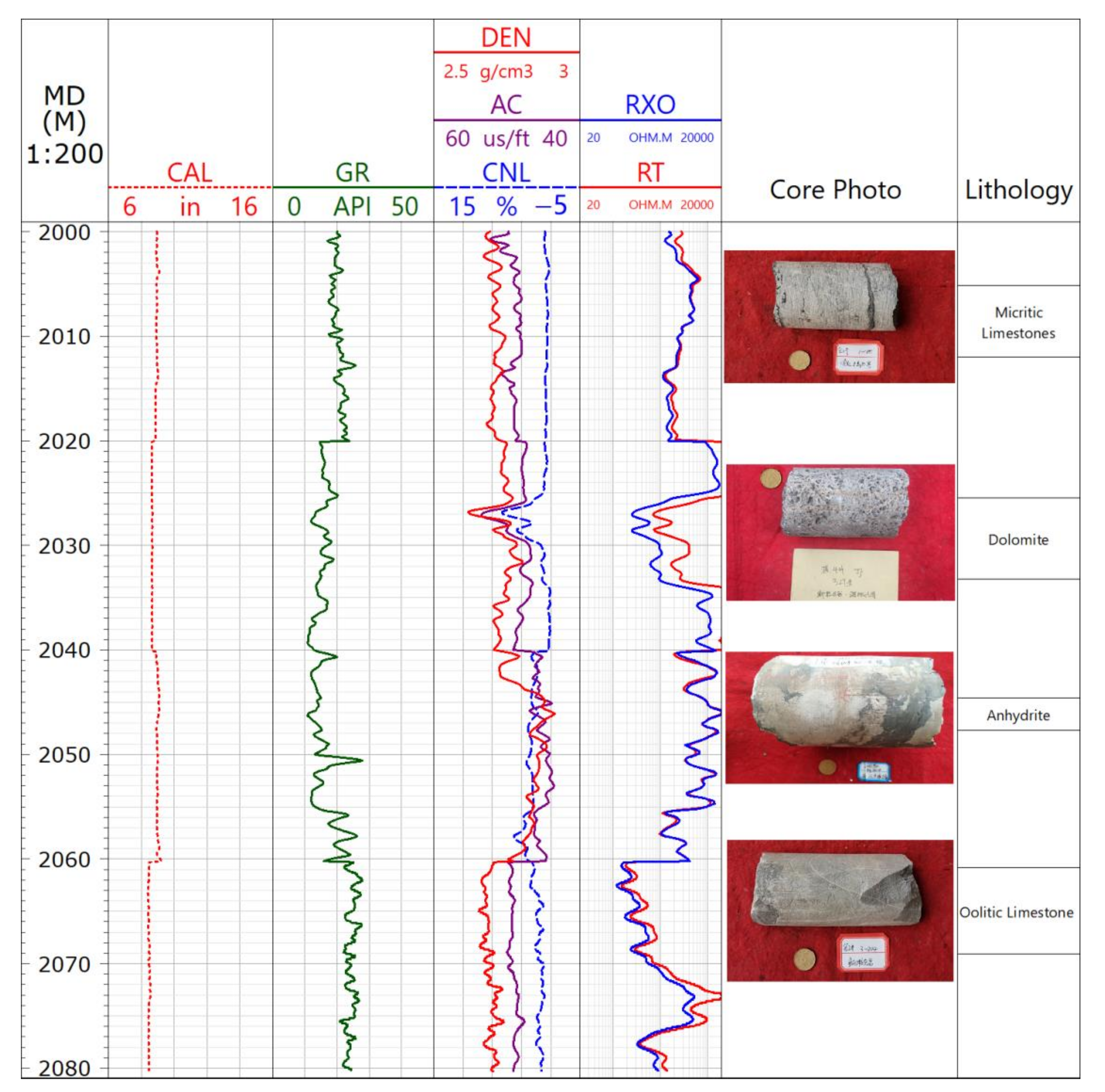
2. Basic Characteristics and Logging Response of the Feixianguan Formation Reservoir
3. Pseudo-Curve Reconstruction Method
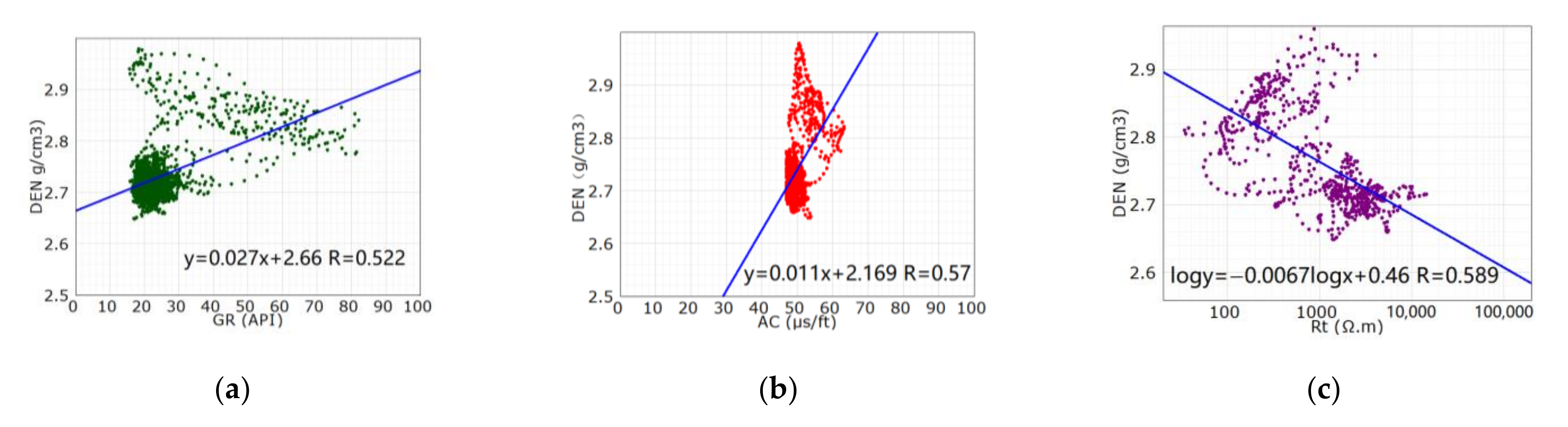
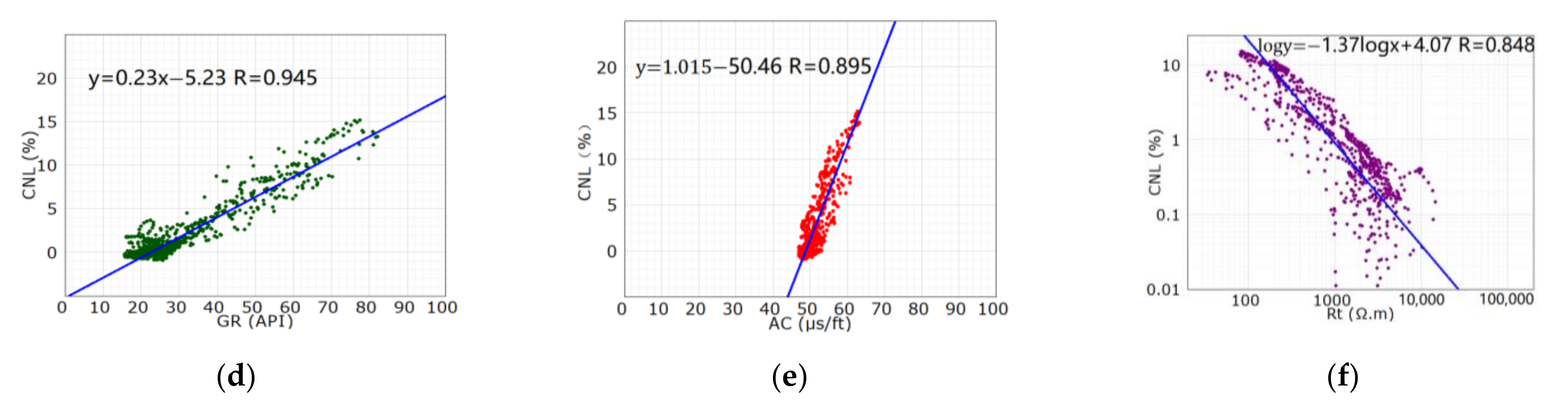
3.1. Selection of the Reconstruction Curves
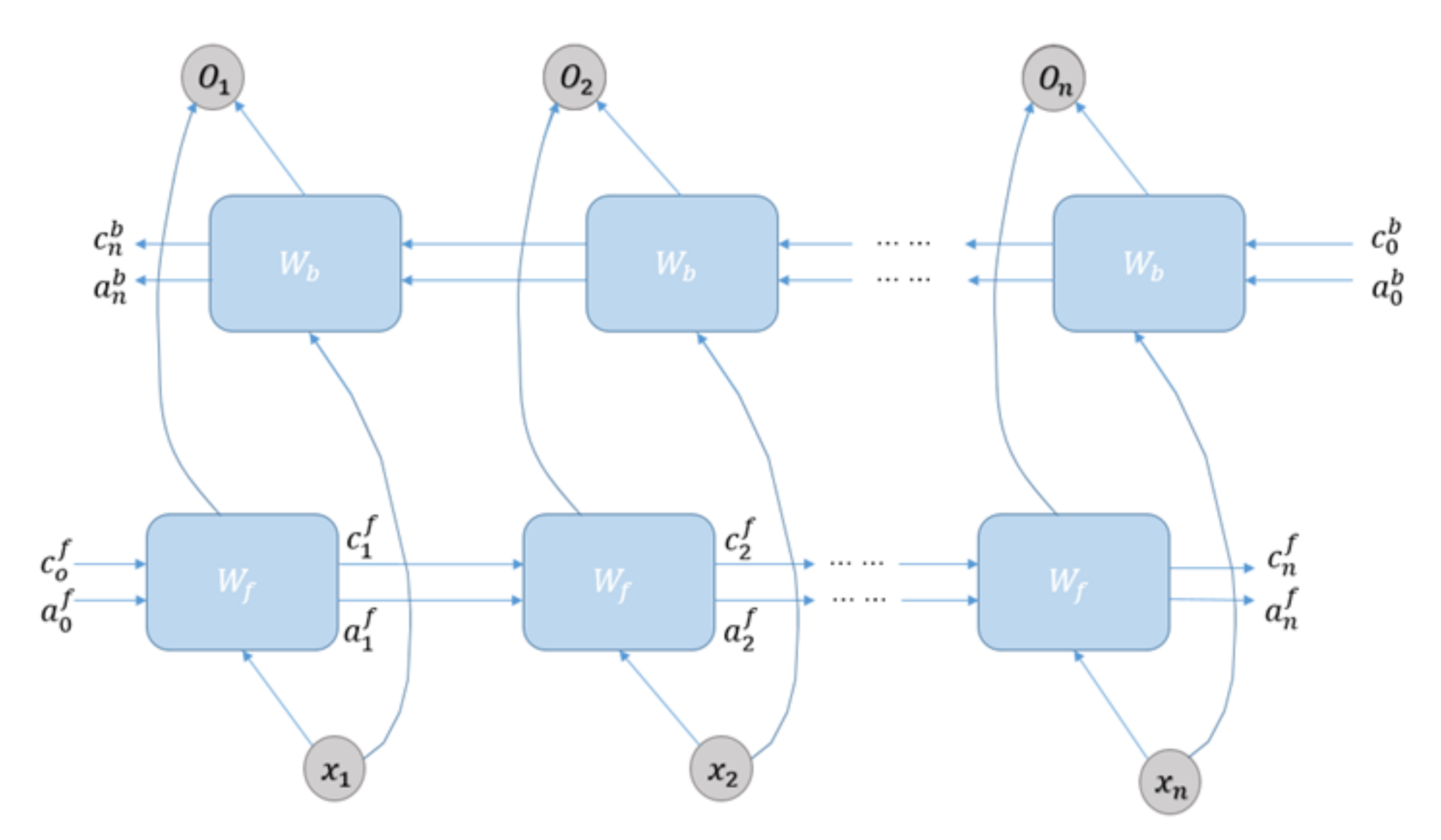
3.2. Selection of Construction Method
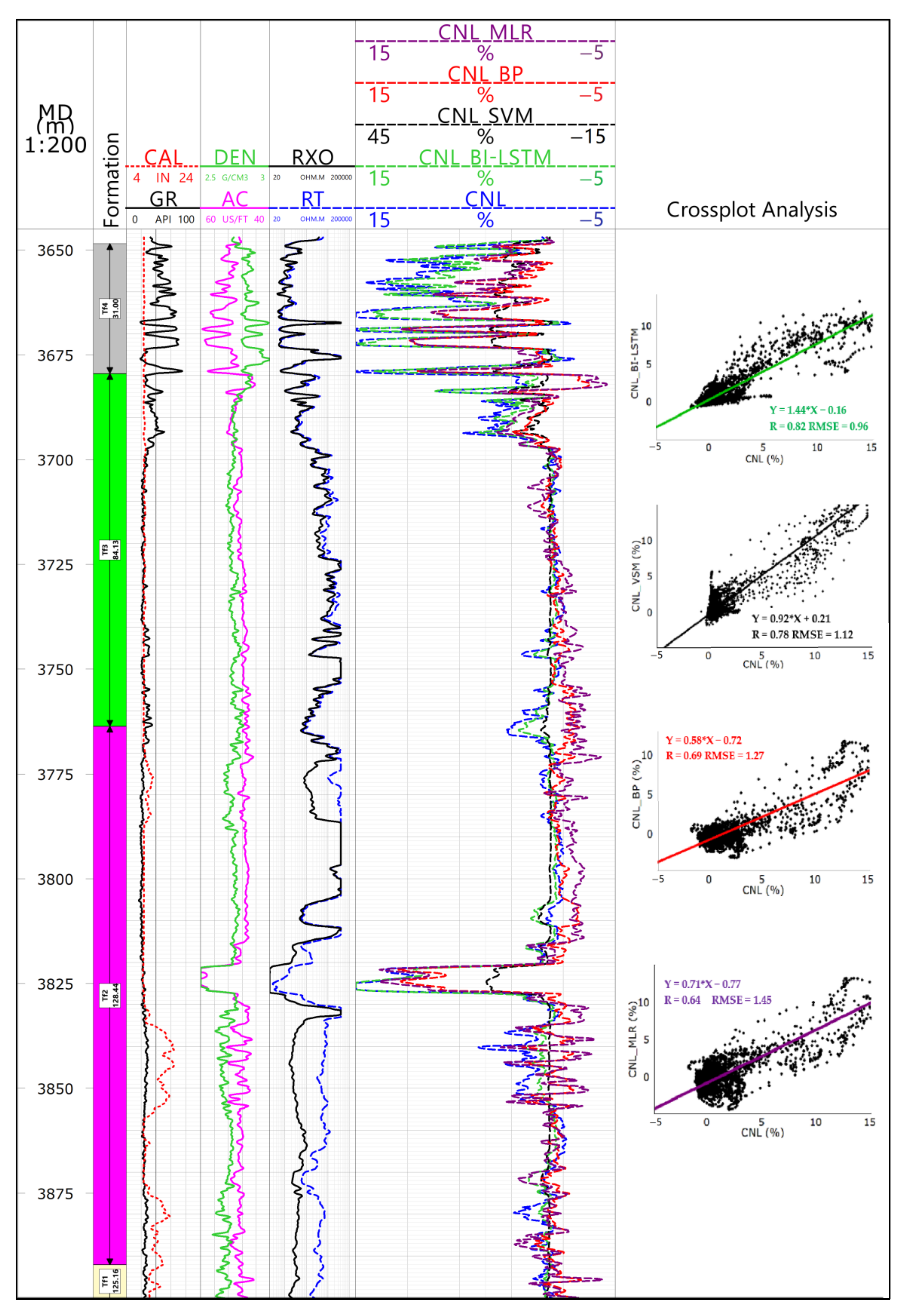
3.3. Pseudo-Curve Reconstruction Experiment
3.4. The Impact of Data Volume on Predicted Results
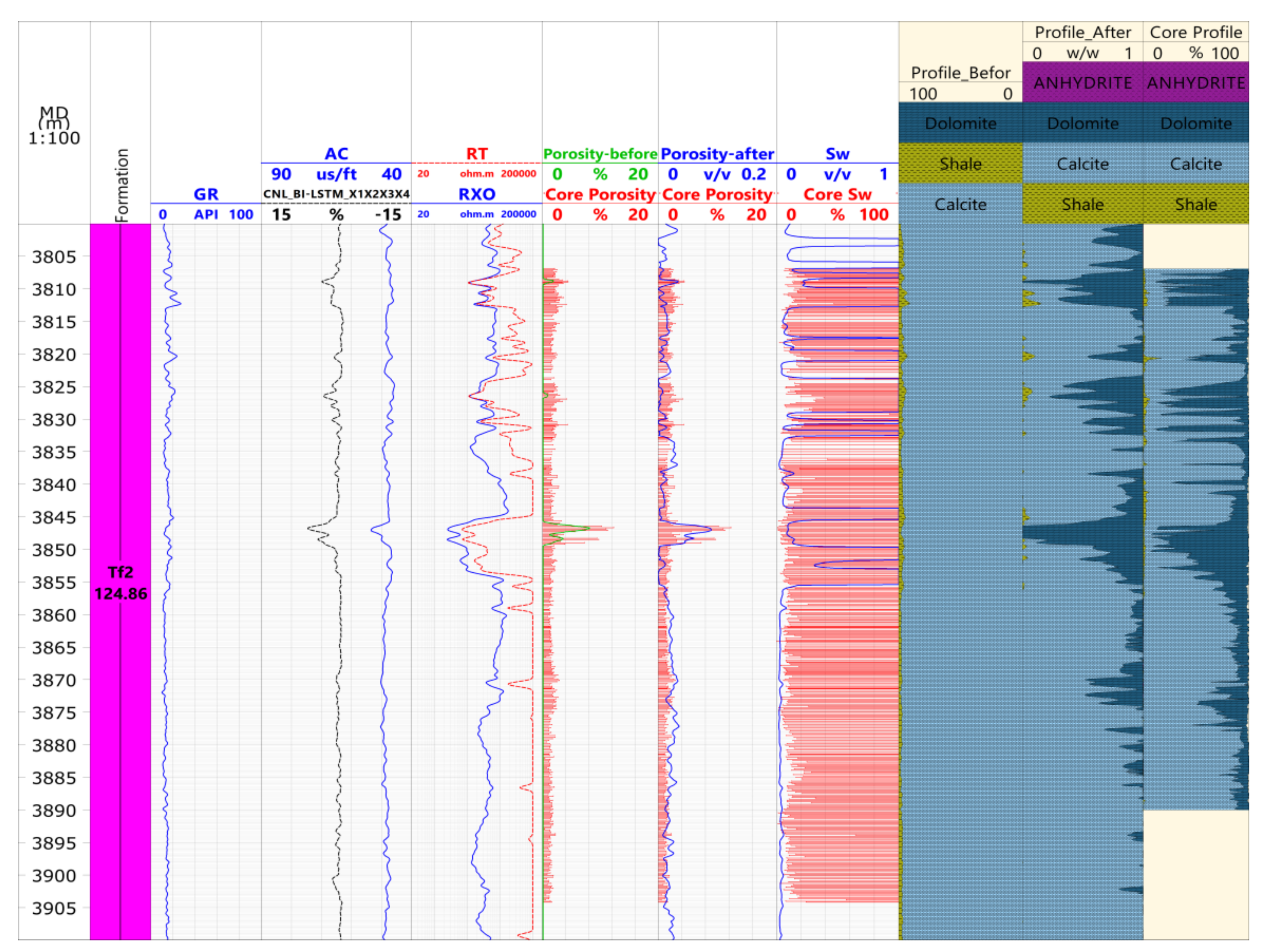
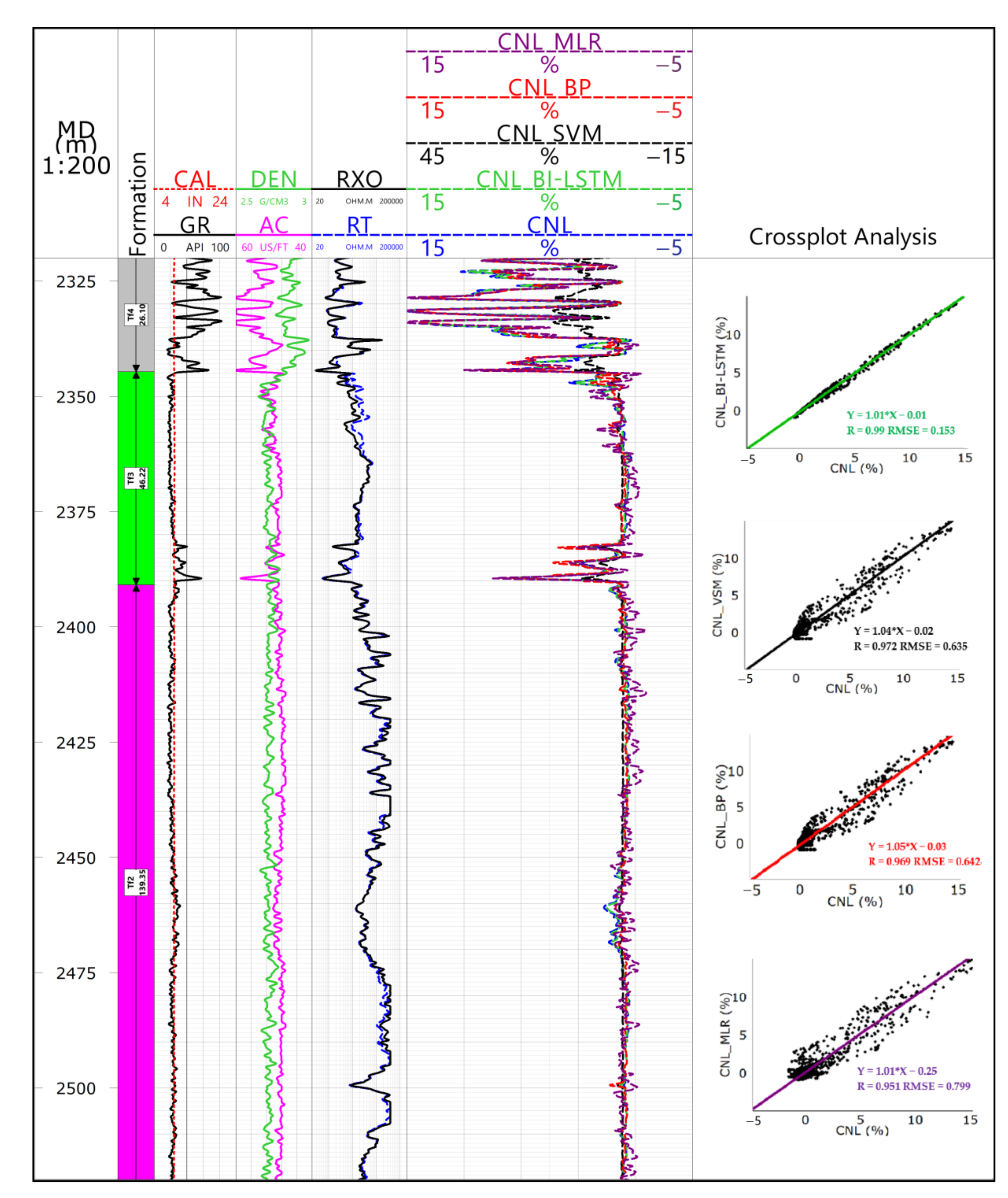
4. Application Effect Analysis
5. Conclusions
- (1)
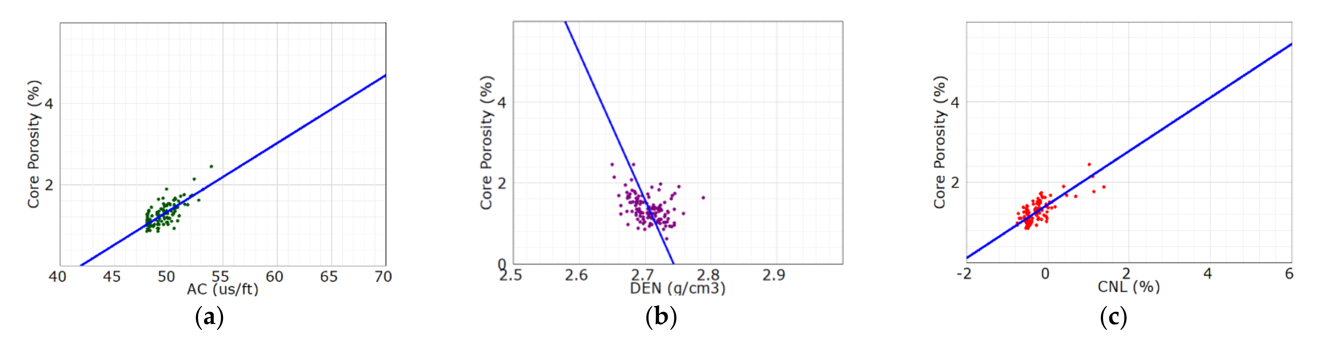
- According to the correlation analysis of the core physical property and the 3-porosity curve in the Feixianguan Formation, the CNL curve is most significantly correlated with the core porosity, less with the AC curve and the least with the DEN curve. The results show that, compared with the DEN curve, in constructing the pseudo-curve, the CNL curve is a more rational choice.
- (2)
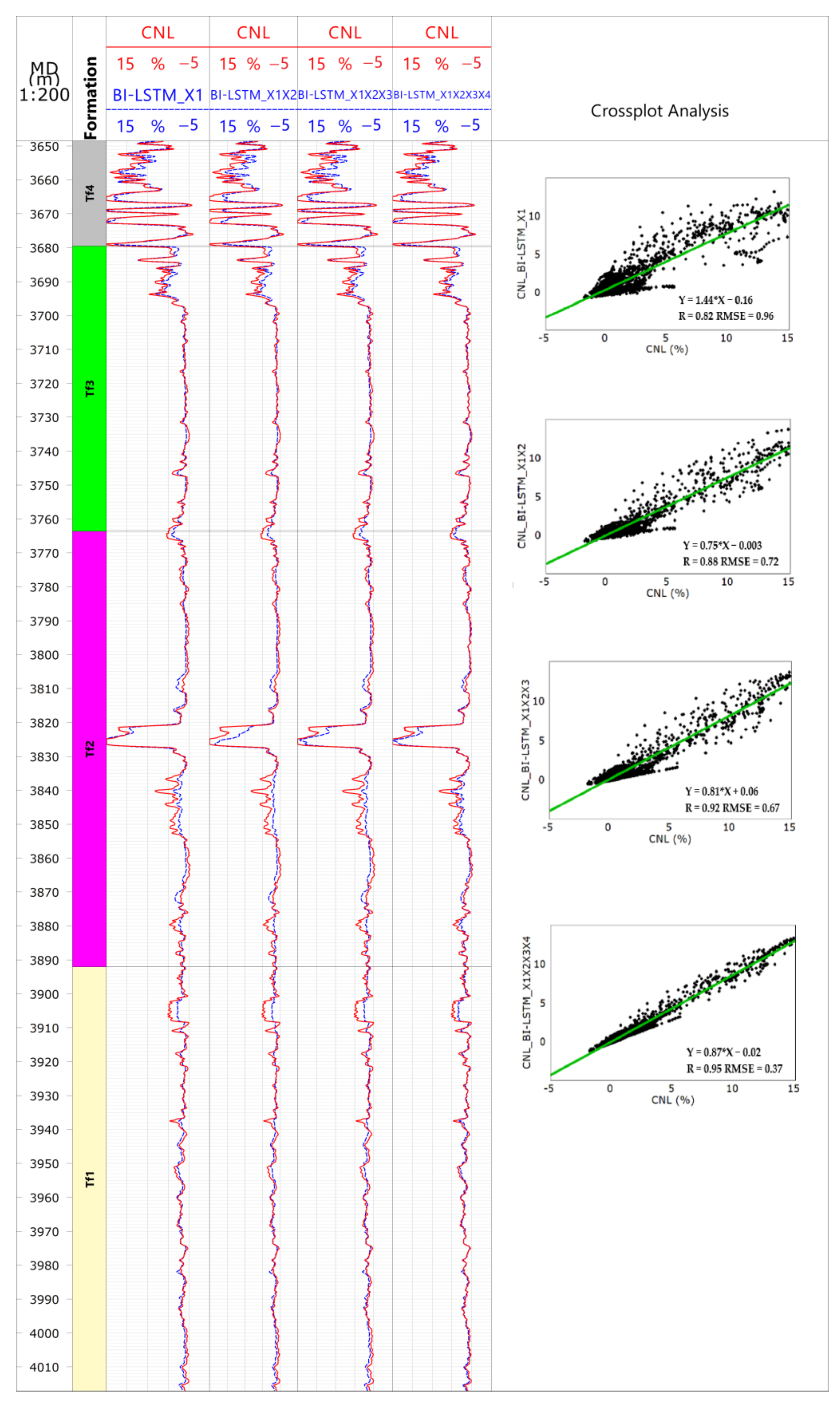
- Compared with the traditional method, BI-LSTM shows greater advantages. This method not only gives full consideration to the interdependence of the sample sequences in the logging depth domain, but also improves the construction precision and accuracy of the pseudo-curve by increasing the amount of data.
- (3)
- With the increase of the amount of training data, the prediction accuracy of the pseudo-curve constructed by BI-LSTM is gradually improved. Yet it is worth noting that BI-LSTM is not affected by the data amount solely.
- (4)
- By using BI-LSTM, the accuracy of the old well pseudo-curve is improved. However, it is suggested that the neutron curves should be standardized before being used for logging data processing and interpretation, and the weight coefficient should be reducing when using the curves.
Author Contributions
Funding
Institutional Review Board Statement
Informed Consent Statement
Data Availability Statement
Conflicts of Interest
Abbreviations
| AC | acoustic |
| GR | natural gamma ray |
| Rt | true formation resistivity |
| Rxo | flushed zone formation resistivity |
| CNL | compensated neutron logging |
| DEN | density |
| Tf1~Tf4 | 1st~4st member of Feixianguan Formation |
References
- Liu, Y.T. Reservoir characteristics of Changxing-Feixianguan Formation in northeastern Sichuan area. Lithol. Reserv. 2019, 31, 78–86. [Google Scholar]
- Wei, G.; Yang, W.; Liu, M.; Xie, W.; Jin, H.; Wu, S.; Su, N.; Shen, J.; Hao, C. Distribution rules, main controlling factors and exploration direction of giant gas fields in the Sichuan Basin. Nat. Gas Ind. B 2020, 7, 1–12. [Google Scholar] [CrossRef]
- Jin, Y.J.; Zhang, Q.; Wang, M.M. Well logging curve reconstruction based on genetic neural network. Prog. Geophys. 2021, 36, 1082–1087. [Google Scholar]
- Liu, J.W.; Liu, Y.; Luo, X.L. Research and development on deep learning. Appl. Res. Comput. 2014, 31, 1921–1930. [Google Scholar]
- Zhao, J.L.; Li, G.; Ma, P.S.; Gong, Z.W.; Meng, L.F.; Li, G. The application of network technology to petroleum logging interpretation. Prog. Geophys. 2010, 25, 1744–1751. [Google Scholar]
- Qin, T.; Cai, J.Y.; Li, D.Y. Application of curve reconstruction technology in accurate reservoir prediction in Bohai Q oilfield. Comput. Tech. Geophys. Geochem. Explor. 2018, 40, 330–336. [Google Scholar]
- Salehi, M.M.; Rahmatii, M.; Karimnezhad, M.; Omidvar, P. Estimation of the non records logs from existing logs using artificial neural networks. Egypt. J. Pet. 2016, 26, 957–968. [Google Scholar] [CrossRef] [Green Version]
- Li, T.T.; Chen, J.R.; Guo, Y.; Pang, X.Y. A reservoir prediction application of density curve reconstruction in complex geological conditions. China Manganese Ind. 2019, 37, 19–23. [Google Scholar]
- Yu, J. Research on reservoir prediction technology based on curve reconstruction. Mod. Chem. Res. 2018, 11, 88–89. [Google Scholar]
- Duan, Y.X.; Li GT Sun, Q.F. Application of convolutional neural network in reservoir prediction. J. Commun. 2016, S1, 5–13. [Google Scholar]
- Yang, B.; Kuang, L.C.; Sun, Z.C.; Shi, J.C. Neural Network and Its Application in Petroleum Logging; Petroleum Industry Press: Beijing, China, 2005; pp. 94–98. [Google Scholar]
- Li, R.J.; Cui, Y.J.; Xiong, L. Evaluating conglomeratic sandstone reservoir in block C of Bohai oilfield by reconstructing neutron log. Well Logging Technol. 2019, 43, 427–433. [Google Scholar]
- An, P.; Cao, D.P.; Zhao, B.Y.; Yang, X.L.; Zhang, M. Reservoir physical parameters prediction based on LSTM recurrent neural network. Prog. Geophys. 2019, 34, 1849–1858. (In Chinese) [Google Scholar]
- Yang, Z.L.; Zhou, L.; Peng, W.L.; Zheng, J.Y. Application of BP neural network technology in sonic log data rebuilding. J. Southwest Pet. Univ. (Sci. Technol. Ed.) 2008, 30, 63–66. (In Chinese) [Google Scholar]
- Zhu, G.J. Application of acoustic curve reconstruction in reservoir prediction. Comput. Tech. Geophys. Geochem. Explor. 2017, 39, 383–387. [Google Scholar]
- Zhou, X.; Cao, J.X.; Wang, X.J.; Wang, J.; Liao, W.P. Acoustic log reconstruction based on bidirectional gated recurrent unit neural network. Prog. Geophys. 2021, 1–11. Available online: http://kns.cnki.net/kcms/detail/11.2982.P.20210209.1209.009.html (accessed on 29 December 2021).
- Han, B.H.; Wang, F.; Liu, Q.R.; Zhang, C.A. Review of research progress on evaluation of logging reservoir classification methods. Prog. Geophys. 2021, 36, 1966–1974. [Google Scholar]
- Hou, X.L.; Hu, Y.; Li, Y.Q.; Xu, X.H. Rational structure of multi-layer artificial neural network. J. Northeast. Univ. (Sci. Technol. Ed.) 2003, 24, 35–38. [Google Scholar]
- Zheng, Y.Z.; Ye, Z.H.; Liu, X.A.; Zhao, L. Research on prediction method of reservoir physical properties based on deep learning. Electron. World 2018, 10, 23–26. [Google Scholar]
- Wei, L.H.; Guo, J.Y.; Yang, Z.L.; Huang, Y.F. Analysis on key techniques of log constrained lithological inversion. Nat. Gas Geosicience 2006, 17, 731–735. [Google Scholar]
- Cheng, X.; Cheng, Y.X.; Cheng, J.H.; Sun, Q.L. Geophysical logging system based on machine learning and big data technology. J. Xi’an Univ. Pet. (Nat. Sci. Ed.) 2019, 34, 108–116. [Google Scholar]
- Zhou, X.Q.; Zhang, Z.S.; Zhu, L.Q.; Zhang, C.M. A new method for high-precision fluid identification in bidirectional long short-term memory network. J. China Univ. Pet. (Ed. Nat. Sci.) 2021, 45, 69–76. [Google Scholar]
- Alizadeh, B.; Najjari, S.; Kadkhodaie-Ilkhchi, A. Artificial neural network modeling and cluster analysis for organic facies and burial history estimation using well log data: A case study of the South Pars Gas Field, Persian Gulf, Iran. Comput. Geosci. 2012, 45, 261–269. [Google Scholar] [CrossRef]
- Bengio, Y.; Simard, P.; Frasconi, P. Learning long-term dependencies with gradient descent is difficult. IEEE Trans. Neural Netw. 1994, 5, 157–166. [Google Scholar] [CrossRef]
- Hochreiter, S.; Schmidhuber, J. Long short-term memory. Neural Comput. 1997, 9, 1735–1780. [Google Scholar] [CrossRef] [PubMed]
- Hornik, K. Approximation capabilities of multilayer feedforward networks. Neural Netw. 1991, 4, 251–257. [Google Scholar] [CrossRef]
- Zhang, B.L.; Luo, D.T.; Hu, P.; Fan, J.; Jin, C. A well log curve generation method based on deep neural network. Electron. Meas. Technol. 2020, 43, 107–111. [Google Scholar]
- Li, C.B.; Fan, J.F.; Song, X.L. A study on application of deep learning in geology. Jiangsu Geol. 2018, 42, 115–121. [Google Scholar]
- Zhang, D.X.; Chen, Y.T.; Meng, J. Synthetic well logs generation via recurrent neural networks. Pet. Explor. Dev. 2018, 45, 598–607. [Google Scholar] [CrossRef]


| Layer | Lithification Analysis Result | Histogram | |||
|---|---|---|---|---|---|
| Dolomite (%vol) | Calcite (%vol) | Gypsum (%vol) | Clay (%vol) | ||
| Tf4 | 1–70, 25 | 5–98, 52 | 0–55, 4 | 5–40, 15 | 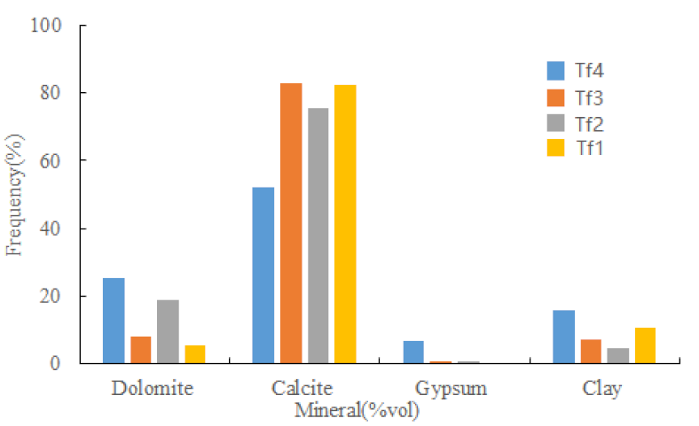 |
| Tf3 | 0–90, 8 | 5–100, 83 | 0–30, 0.5 | 0–30, 7 | |
| Tf2 | 0–98, 18 | 0–100, 75 | 0.75, 0.5 | 0–23, 4 | |
| Tf1 | 0–80, 5 | 0–100, 82 | / | 0–63, 10 | |
| Lithology | Porosity (%) | Typical Logging Response Characteristics | |||||
|---|---|---|---|---|---|---|---|
| GR (API) | AC (μs/ft) | CNL (%) | DEN (g/cm3) | RT/RXO | |||
| Limestone | Oolitic | 1–6 | low, 10–20 | higher, 48–52 | >0 | low, 2.6–2.7 | lower, plus difference characteristic |
| Micritic | 0–1.5 | higher, 15–25 | lower, 47–49 | Near the “0” line | lower, 2.69–2.72 | higher, approximate coincidence | |
| Dolomite | 1.5–12 | low, 10–20 | high, 48–55 | >0 | lower, 2.6–2.8 | low, obvious plus difference characteristic | |
| Anhydrite | 0–1 | low, 10–15 | low, 43–47 | <0 | High, >2.9 | high, approximate coincidence | |
| Data Set | Evaluation Parameter | Method | |||
|---|---|---|---|---|---|
| MLR | BP | SVM | BI-LSTM | ||
| Self-judgment of Training Set X1 | R | 0.951 | 0.969 | 0.972 | 0.99 |
| RMSE | 0.799 | 0.642 | 0.635 | 0.153 | |
| R2 | 0.91 | 0.96 | 0.97 | 0.97 | |
| Examination of Training Set X5 | R | 0.64 | 0.69 | 0.74 | 0.82 |
| RMSE | 1.45 | 1.27 | 1.12 | 0.96 | |
| R2 | 0.46 | 0.58 | 0.66 | 0.71 | |
| Well Name | Evaluation Parameter | BI-LSTM | |||
|---|---|---|---|---|---|
| Training Set X1 | Training Set X1X2 | Training Set X1X2X3 | Training Set X1X2X3X4 | ||
| Test Set X5 | R | 0.82 | 0.88 | 0.92 | 0.95 |
| RMSE | 0.96 | 0.72 | 0.67 | 0.37 | |
| R2 | 0.71 | 0.76 | 0.78 | 0.79 | |
| Comparative Analysis of Porosity | Average (%) | Correlation Coefficient | Absolute Error (%) | Relative Error (%) |
|---|---|---|---|---|
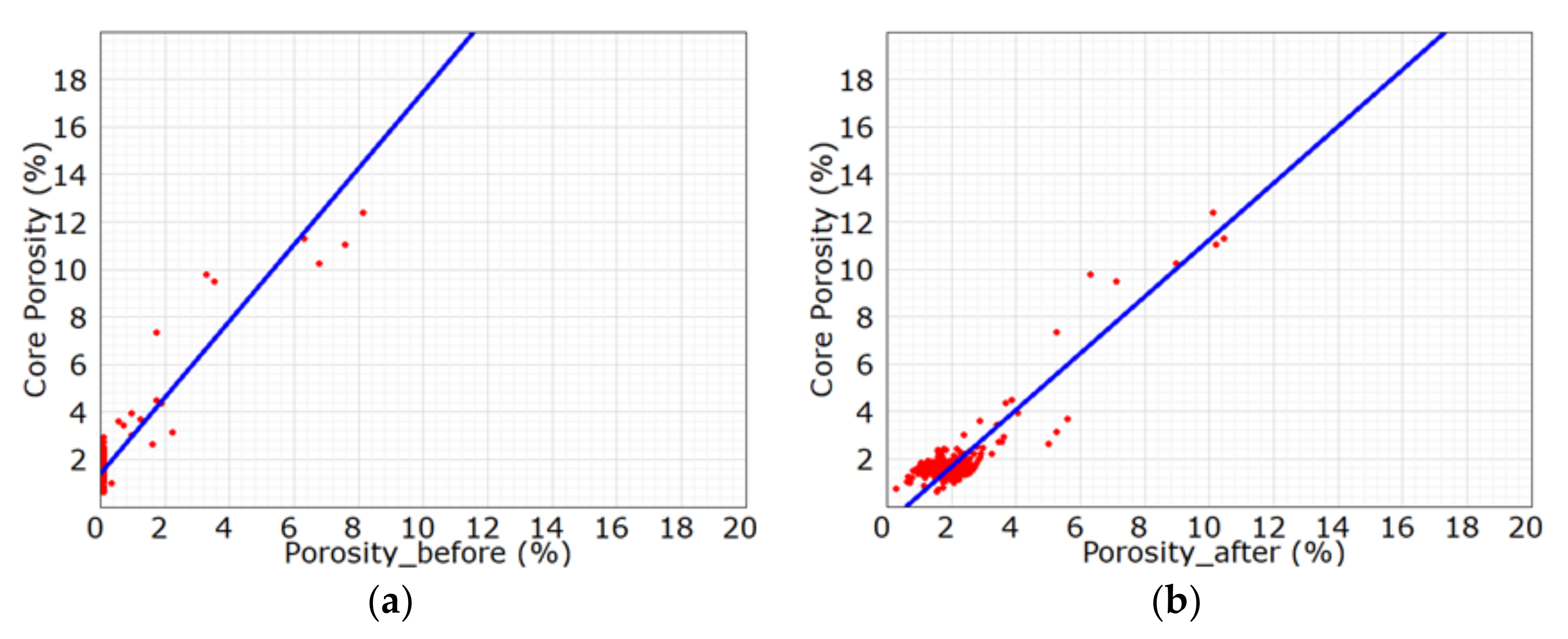
| Core porosity | 1.90 | \ | \ | \ |
| Porosity before | 0.30 | 0.815 | 1.6 | 84.2 |
| Porosity after | 2.18 | 0.896 | 0.28 | 14.7 |
Publisher’s Note: MDPI stays neutral with regard to jurisdictional claims in published maps and institutional affiliations. |
© 2022 by the authors. Licensee MDPI, Basel, Switzerland. This article is an open access article distributed under the terms and conditions of the Creative Commons Attribution (CC BY) license (https://creativecommons.org/licenses/by/4.0/).
Share and Cite
Cheng, C.; Gao, Y.; Chen, Y.; Jiao, S.; Jiang, Y.; Yi, J.; Zhang, L. Reconstruction Method of Old Well Logging Curves Based on BI-LSTM Model—Taking Feixianguan Formation in East Sichuan as an Example. Coatings 2022, 12, 113. https://doi.org/10.3390/coatings12020113
Cheng C, Gao Y, Chen Y, Jiao S, Jiang Y, Yi J, Zhang L. Reconstruction Method of Old Well Logging Curves Based on BI-LSTM Model—Taking Feixianguan Formation in East Sichuan as an Example. Coatings. 2022; 12(2):113. https://doi.org/10.3390/coatings12020113
Chicago/Turabian StyleCheng, Chao, Yan Gao, Yan Chen, Shixiang Jiao, Yuqiang Jiang, Juanzi Yi, and Liang Zhang. 2022. "Reconstruction Method of Old Well Logging Curves Based on BI-LSTM Model—Taking Feixianguan Formation in East Sichuan as an Example" Coatings 12, no. 2: 113. https://doi.org/10.3390/coatings12020113
APA StyleCheng, C., Gao, Y., Chen, Y., Jiao, S., Jiang, Y., Yi, J., & Zhang, L. (2022). Reconstruction Method of Old Well Logging Curves Based on BI-LSTM Model—Taking Feixianguan Formation in East Sichuan as an Example. Coatings, 12(2), 113. https://doi.org/10.3390/coatings12020113