Considering Thermal Diffusivity as a Design Factor in Multilayer Hybrid Ice Protection Systems

Abstract

Icing is a major problem that affects the aeronautical sector, which is forced to use anti- and de-icing systems to ensure flight safety. The currently used systems are effective but exhibit high energy consumption. Resistive heating is used to prevent ice accretion or to release it once it has formed. To satisfy all the imposed airworthiness requirements, such as low aerodynamic impact, resistance to lightning strikes, no overheating, etc., multilayer systems are commonly configured with different layers fulfilling specific functions. For example, the Boeing 787 Dreamliner uses dry woven glass fiber fabric on top of the heating element to provide galvanic insulation and dielectric resistance. It satisfies the above-mentioned requirements, but its thermal conductivity is very low, therefore reducing energy efficiency. The thermal distribution of two materials (AA6061 aluminum alloy and PTFE) with significantly different thermal and electrical properties in contact with a heating element was studied. Finite element calculations and experimental testing in an icing wind tunnel were carried out at −12 °C under different convection conditions: natural (0 m/s) and forced (35 and 70 m/s), using specimens of different sizes. Heating elements areas were also varied. AA6061 showed homogeneous heating, whereas differences of up to 80 °C were observed when using PTFE. In addition, the test results highlighted the effect of forced convection and the need to evaluate these systems “in close to operative” conditions. The calculation results proved to it be an interesting tool for studying the behavior of the systems avoiding extensive testing.

1. Introduction

The excessive accretion of ice on structures exposed to icing conditions is a serious issue for various industrial sectors such as aviation [1] and power generation [2] or distribution [3]. For this reason, in recent decades, considerable efforts have been made toward the understanding of ice formation and accumulation processes [4,5,6,7,8,9,10,11,12].

Nowadays, the most reliable and common way to fight against ice build-up is the use of active ice protection systems (IPSs), such as de-icing boots, electrothermal mats, or hot air bleeding. These systems can be used in anti-icing mode to avoid ice accretion or facilitate its detachment or, in de-icing mode, to release ice once it has accreted.

One of the main goals of thermal icing protection systems (IPS) is to heat an area minimizing the power consumption and the heating time. There are several general guides proposed by Heinrich et al. [13] for electrothermal IPSs for aviation purposes. For example, in de-icing mode systems, the energy used should be carefully controlled if too much heat is supplied; ice can appear in other areas as a consequence of water flow and refreezing (known as runback ice). On the other hand, if not enough heat is provided, a thick ice layer will form, reducing aerodynamic efficiency and compromising the safety of the operation. Common criteria [14] define 5–10 °C and 50 °C as the operating temperatures for “anti-icing and de-icing modes”, respectively.

The time needed to reach the desired temperatures is another critical constraint that could seriously affect ice accretion rates and, therefore, safety, as well as total energy consumption.

As shown in recent studies, the combination of an active system (which needs an energy supply) and a passive system (which does not), so-called hybrid systems, proves to decrease the energy consumption [15,16] of the overall protection system [3].

However, as in any other high tech-industry, aeronautic devices perform various tasks simultaneously, and currently used electrothermal protection systems are no exception. For aeronautical requirements, a complex architecture is needed at the surface, including layers with different functionalities [17]: thermal insulation, resistive heating, dielectric resistance in case of lightning strikes [18], erosion shielding, etc. However, just a few of the reported studies considered thermal conductivity or diffusivity in the different system layers [19,20]. For example, Wright and collaborators from NASA modeled the surface temperature of multilayered airfoils, aiming to improve active anti-icing systems [18]. In addition, Strehlow and Moser [20] highlighted the importance of minimizing the thermal interference between the heating element and the leading edge skin and obtained a 24% savings in energy consumption by improving the bonding of layers. Huang et al. [21] described the properties required for coatings to be effective alone or as part of a hybrid de-icing system. High thermal conductivity is emphasized as a key property in dedicated active thermal elements or layers mainly due to its correlation with thermal spatial uniformity.

Uniform energy distribution is needed to avoid overheating or local ice formation in cold spots, as IPSs are usually constructed using resistive wires, which provide heat locally. Huang and collaborators [21] also concluded that conductivity is not commonly studied in coatings or layers with different purposes. Mohseni and Amirfazli optimized the distance between heating wires to obtain the target temperature along the chord of a NACA 0021 profile based on the low thermal conductivity of composite material [22]. This design was successful for anti-icing purposes, but thermal homogeneity was not achieved.

The design of more efficient electrothermal active and hybrid IPS is desired, and the thermal diffusivity of the different layers that constitute the systems needs to be considered as a relevant design factor. Multiple parameters and the need for testing the systems under real icing, or at least forced convection conditions, would result in very complex testing matrixes. In addition, the experimental conditions are not easily reproducible in the laboratory, and icing wind tunnel (IWT) tests are expensive. For this reason, system modeling and numerical resolution methods of the corresponding constitutive equations would make the designing much easier and at a lower cost, allowing us to optimize parameters in a theoretical way and then confirm their behavior in an experimental way.

The aim of this work is to study the influence of the thermal properties of different materials in the temperature distribution obtained from a heater working in anti-icing mode temperatures (5–10 °C) during a short activation time stage (30–40 s). The specific objectives are:

• To study how the temperature is distributed along two highly different thermal behavior material layers (a metal and a polymer) in terms of temperature homogeneity and response time.
• To evaluate natural and forced convection thermal effects in an electrothermal IPS.
• To develop finite element modeling tools for the design of active IPS on the basis of thermal distribution.
• To determine the advantages and limitations of the use of high or low thermal diffusivity layers as part of a multilayered system for anti-icing purposes.

For these tasks, thermographic studies have been carried out in natural (wind speed = 0 m/s) and forced convective conditions (35 and 70 m/s), at −12 °C in an IWT, to evaluate the effect of a resistive element, on 1.5 mm thick coupons of aluminum 6061 alloy and pure Polytetrafluoroethylene (PTFE), given that both materials have very different Thermal conductivities and similar, or at least in the same magnitude, density, and specific heat capacity. Reducing, this way, the differences in thermal diffusivity related to anything rather thermal conductivity.

Different specimen sizes and power densities were experimentally studied. In parallel, a finite element method (FEM) simulation has been undertaken in order to allow parameter optimization without extensive experimental testing.

2. Materials and Methods

2.1. Materials

Two materials with different thermal conductivities but similar densities were used (

Table 1. Thermal properties of tested materials.

Material	Density (kg/m3)	Specific Heat Capacity (J kg−1 K−1)	Thermal Conductivity (W m−1 K−1)	Thermal Diffusivity (m2 s−1)
PTFE [23]	2200	1500	0.3	9.09 × 10−8
AA6061 [24]	2700	897	205	8.46 × 10−5
Steel [23]	8050	490	45	1.14 × 10−5

):

• AA6061 T6 (0.66% Si, 0.11% Mn, 0.18% Cr, 0.23% Cu, 0.41% Fe, 0.86% Mg, 0.06% Zn, and 0.03% Ti) provided by ThyssenKrupp Materials Ibérica (Martorelles, Barcelona, Spain).
• PTFE sheets acquired from J. Morell S.A (Tarragona, Spain)

The heating elements were made of 18 Cr 9 Ni steel sheets (Record Metall-Folien GmbH, Mühlheim am Main, Germany) with a thickness of 50 microns and were cut at 60 mm × 5 mm, in order to cover the 50 mm width of the specimen and leaving 5 mm at each side for electrical connections. The effective heating area was taken as 50 mm × 5 mm.

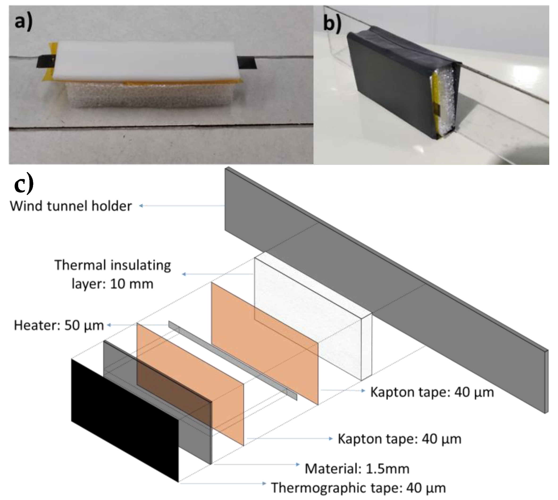
2.2. Icing Wind Tunnel Test

The tests were carried out at INTA’s IWT, a small-scale wind tunnel placed inside a climatic room with a 15 cm × 15 cm testing chamber. The wind speed can be controlled from 20 to 70 m/s, and the temperature can be set between the ambient T to −20 °C. More details of INTA’s IWT are described elsewhere [25,26,27].

Test specimens were placed perpendicular to the airflow at −12 °C and attached to a fixture within the wind tunnel. The test coupons were placed over the heating element longitudinally (see Figure 1a). Kapton tape (40 mm) from © tesa SE (Hamburg, Germany) was used as an electrical insulator. For PTFE, it is not required, but it was used nevertheless in order to compare both materials under the same conditions.

A 1 cm thick polyethylene foam layer was located below the heater as a thermal insulator to minimize thermal diffusion in that direction (see Figure 1). This configuration is typical in electrothermal applications [28,29,30] using thermal insulator materials such as synthetic rubber.

A Testo 890 thermographic camera (Testo SE & Co. KGaA , Titisee-Neustadt, Germany) was used to monitor the surface temperature, and the system was covered, as recommended by the manufacturer, with a high IR emissivity tape (Tesaflex^® 53988, © tesa SE (Hamburg, Germany). The processing of the data was carried out with the IRsoft software (version 4.3).

The specimens were cooled to −12 °C in the climatic room prior to testing.

The IRSoft software, employed for thermographic data measurement, allows exporting of thermal information for every pixel. Counting the number of pixels at T higher than 5 °C relative to the total number of pixels composing the surface, the surface percentage can be calculated.

Composition, properties, and thermal homogeneity of the commercial materials were assumed, and just one sample of every material and size was used. However, each condition was tested 5 times finding very low dispersion in results among them. A representative curve of every testing condition was used for the analysis.

2.3. Thermal FEM Model Tests

To understand the effects of thermal conductivity and diffusivity of each material, a heat transfer model was applied to find a transient solution of the heat equation:

$$\nabla \left(q\left(r,t\right)\right)+{\dot{e}}_g\left(r,t\right)=\frac{\rho C_p\partial T\left(r,t\right)}{\partial \mathrm{t}}$$

(1)

With:

${\dot{e}}_g$: Volumetric generation rate (W/m³)

$q$: Heat flux (W/m²)

$\rho$: Solid density (kg/m³)

$C_p$: Solid Specific heat (J kg⁻¹ K⁻¹)

$r:$Variable of space (m)

$t:$ Variable of time (s)

This model establishes that the heat losses due to radiation are negligible.

The Code Aster solver software (version 10.2) [30] was used with a discretization of time and space in order to calculate the temperatures as a function of time and position of the specimens. The time discretization was made with a finite differences method, and the space discretization was conducted through both three-dimensional and bidimensional FEM models (Figure 2).

In the case of the 3D model, a tetrahedral mesh was implemented due to its simplicity, and for the 2D model, a triangular structured mesh was applied. Meshes with different element sizes depending on the substrate layer were checked, choosing a size that accurately represents the temperature profile along the thickness. The results between the 3D and the 2D thermal model were compared in order to establish that the simplification was appropriate. The solutions of both models are similar, with a lower computational time for the 2D model. However, real anti-icing systems are not bidimensional, having complex geometries, so a 3D model should be applied.

3. Results and Discussion

For all experiments, a temperature of 5 °C was chosen, as it is the critical temperature that must be reached for the IPS to accomplish its function.

In order to specify the terminology used in this study, the following terms are defined:

• Heating surface as the area of the heating resistance that provides heat to the system, in this case, 50 mm × 5 mm.
• Heated surface as the specimen size. Three different sizes were studied (50 mm × 25 mm, 50 mm × 12.5 mm, and 50 mm × 5 mm).
• Cold spot (CS) as the pixel or point with the lowest measured temperature in the studied surface.
• Hot spot (HS) as the pixel or point with the highest measured temperature in the studied surface.

For the purpose of comparing the behavior of AA6061 and PTFE, four parameters were used:

Temperature (T): the thermographic camera registers T in every pixel of the surface. Profiles were taken crossing the center of the specimen (Figure 3, P1 line). To avoid edge effects, the measurement area excludes the top and bottom 2 mm of each sample. Temperature profiles which include both the heating element and the specimen boundaries, as well as the measurement area, are shown in Figure 3c,d.

Two key temperatures were measured within the heated area: the HS generally at the center of the specimen and the CS at the highest distance from the heater.

Specimen surface over 5 °C (%): calculated as the specimen surface with T ≥ 5 °C /total specimen surface. T is measured by means of the thermographic camera.

Activation time: defined as the time required for an IPS surface to reach 5 °C. Activation time can be measured for different surface points, e.g., HS activation time and CS activation time.

Power consumption / Electric energy consumption: based on the heating element power at different modes and times. This can be represented in three ways:

• Total instantaneous power (W).
• Power density (W/cm²): total instantaneous power/specimen area.
• Energy consumption (J/cm²): energy consumed during heating calculated by the following formula:

$$e\approx P_{elec}{t}_f$$

(2)

where e is the power consumption, $P_{elec}\left(t\right)$ the total instantaneous power, and $t_f$ the required time for the specimens to reach 5 °C.

The tests were designed to study the influence of the material thermal properties in transverse and longitudinal heating, the effect of forced convection, and the ratio of heated surface relative to the heating element surface.

3.1. Temperature Homogeneity

This test determines the behavior of both materials when heated from −12 °C to 5 °C under natural convection conditions by measuring the temperature as a function of time. A constant power input of 10.9 W was chosen using 25 × 50 mm² specimens.

The thermal homogeneity of the heating element was checked. More details can be found in the supporting information (Figures S1–S6).

As expected, uniform temperature distribution was observed on the AA6061 specimens due to its high thermal diffusivity, as shown in Figure 4, especially when compared with heating PTFE, where the specimen zones close to the heater reached higher temperatures considerably faster than areas away from it.

After 42 s all the AA6061 surface is higher than 5 °C, while in PTFE, only 26% has reached this temperature (or higher). The calculation has been made with the number of pixels above 5 °C in a given time (avoiding the area of the clamps and outside the test specimen) and referenced to the total pixels of the specimen area.

Figure 5 and Figure 6 show temperature profiles taken across line P1 (Figure 3) as well as simulated profiles obtained by FEM for AA6061 and PTFE as a function of time elapsed since the heating element was turned on.

The temperature profile for 180 s in Figure 6 left is flattened in the central part because the IR thermographic camera sensor was set from −30 to 100 °C, and the measurement exceeds that value.

The FEM model calculations and the experimental results reasonably match in terms of temperature distribution and maximum temperature as a function of time. The main difference is the minimum temperature in the PTFE profiles. Even after long time periods, the areas near specimen boundaries’ simulated temperatures are always below 0 °C, while the experimental data indicate T > 0 °C after 120 s. This difference could be attributed to a redistribution of the dissipated heat from the heated surfaces to the rest of the surface by means of convection through heated air.

Geometrical variables such as substrate geometry and heating element dimensions, as well as the materials’ thermal properties such as diffusivity and conductivity, will have strong effects on the temperature distribution. In addition, for the FEM calculations, boundary conditions such as the system’s thermal insulation or convection are critical as well. The thermal insulation was modeled in two ways: (a) considering an adiabatic boundary condition in the substrate internal layer and (b) creating the geometry and applying to the thermal insulation layer a low conductivity value (this was used in the 3D calculation model).

Another interesting parameter that defines the thermal performance of an electrothermal IPS is the surface % that has reached a specific temperature ≥ than the target temperature (5 °C). This ratio could be interesting in some cases. Even though the surface is not fully protected, there are areas that are not so critical and do not require protection, accumulating heat in some specific critical regions. This happens, for example, on airfoils, where leading edges are protected with an anti-icing mode, but downstream only the de-icing mode is needed [31].

In Figure 7, it can be observed that using the same heating parameters at the time required for the whole aluminum surface to reach 5 °C or higher (42 s), only 26% of the PTFE surface is above 5°.

Regarding the comparison of the experimental surface heating with the FEM model data, the results of surface percentage at temperature ≥ 5 °C can be seen in Figure 8.

A good agreement is found as the FEM model indicates that 41 s are needed to heat all the AA6061 aluminum area to 5 °C or above, whereas 42 s were measured experimentally. The same trend was observed for PTFE as the experimental data indicated that 26% of the PTFE area was above 5 °C after 42 s while the model predicted 25.86%. AA6061 reaches 5 °C abruptly due to very homogeneous heating. On the other hand, in the case of PTFE, the heating rate is slower.

3.2. Effect of Convection

To observe the effect of convection on the surface temperature, tests were carried out at the same power for different specimen sizes for the two chosen materials. Their temperature was measured for different air speeds: 0 m/s (natural convection), 35 m/s, and 70 m/s (forced convection).

As expected, the power needed to satisfy the 5 °C requirements for natural or forced convection conditions was different, as shown in

Table 2. Matrix of power consumption at different air speeds and for different heated areas.

Air speed (m/s)	Power (W)	Power Density (W/cm2)
		50 × 25 mm	50 × 12.5 mm	50 × 5 mm
0	10.9	0.872	1.744	4.36
35	24.2	1.936	3.872	9.68
70	33.6	2.688	5.376	13.44

.

The natural convection boundary condition, without an incident airflow, is defined with a constant convection heat transfer coefficient. Typically, 10 W/m² is used [28] in order to calculate the temperature transitory profile of an electrothermal multilayer IPS. In the model, different natural convection heat transfer coefficients with values of less than 10 were used, with very similar solutions in the transient part of the solution.

The convection heat transfer coefficient calculation is complex, so several studies use experimental methods in order to approximate its value [32,33,34]. For example, Samad et al. [32] calculated the convective heat transfer coefficient from the temperature values that were taken in a heated airfoil located in an IWT. Guoqiang et al. [33] studied the influence of using a constant Nusselt number in the calculation of the convective heat transfer coefficient ($N{u}_x=h\left(x\right) x/k)$ for an airfoil and for different airflow conditions. The experimental results were compared with the analytical Nusselt number, having accurate results. Experimental methods cannot be used in this particular geometry and wind conditions, so analytical values must be used.

A key parameter, such as the convective heat transfer coefficient, is difficult to calculate analytically. Usually, in Ice Prediction Software such as LEWICE or ONERA, the convective heat transfer coefficient is calculated with an integral boundary layer method. Traditionally, for this type of method, constant temperatures all over the surface are assumed when the laminar flow is used [35] in order to simplify the integral boundary layer equation. Recently, ONERA has developed a method in order to include non-isothermal conditions in airfoil and wedge profiles [36].

The heat flux in the surface can be calculated using Equation (3), where St is the Stanton number, Pr the Prandtl number, Re is the Reynolds number, T_s is the substrate surface temperature, k_a is the thermal conductivity of air, $T_{\infty }$the environment temperature, and h(x) is the convective heat transfer coefficient as a function of the distance to the center of the specimen “x”:

$$q_{wall}=\frac{St \mathit{Pr} R{e}_x k_a}{x}\left(T_s-T_{\infty }\right)=h\left(x\right)\left(T_s-T_{\infty }\right)$$

(3)

For the Falkner-Skan [37] solution, the external velocity $u_e$ can be calculated through the geometrical parameter $\beta$. According to the Falkner-Skan solution for a surface perpendicular to the airflow direction, $\beta =1$. If the relationship $u_e\left(x\right)=A{x}^{\frac{\beta }{2-\beta }}=Ax$ is applied and knowing that the Stanton number$St=1/2\sqrt{m/R{e}_x}$ and the Reynolds number is$R{e}_x=u_e x/\nu$, the convective heat transfer coefficient can be calculated using Equation (4):

$$h\left(x\right)=\frac{1}{2}\sqrt{mR{e}_x}\mathit{Pr}\frac{k}{x}=\frac{\mathit{Pr}k}{2}\sqrt{\frac{mA}{\nu }}\approx 200\frac{W}{m K}=constant$$

(4)

In the previous solution, a surface isothermal condition is assumed. In the case of AA6061, as seen before, this condition is satisfied due to its high conductivity, so the convective heat transfer coefficient is accurate and solutions are feasible. In the case of PTFE, this condition is not applicable because there are high temperature variations, so the convective heat transfer coefficient would be variable, and the solution provided by White [35] is not accurate.

For PTFE, an integral method of the boundary layer is needed. The procedure consist in integrating the energy Navier–Stokes equation in the direction perpendicular to the surface. In the following equation, the flow has been considered incompressible, the airspeed normal to the surface is 0 and no-slip conditions on the surface.

$$\frac{d{\delta }_T}{dx}+\frac{{\delta }_T}{T_{wall}-T_{oe}}\frac{d{T}_{wall}}{dx}+\frac{{\delta }_T}{u_e}\frac{d{u}_e}{dx}=St$$

(5)

where ${\delta }_T$ is the thermal boundary layer thickness, x is the distance in the flow direction, $T_{wall}$ is the temperature in the specimen surface, $u_e$ is the airspeed, and $T_{0e}$ is the total temperature. However, for calculating the Stanton number $St=q_{wall}/\left({\rho }_e{u}_e{c}_p\left(T_{wall}-T_{\infty }\right)\right)$, the heat flux in the wall, which depends on the FEM thermal model, must be known. The FEM thermal model provides a relationship between $q_{wall}$ and $T_{wall}$, but it would generate infinite solutions for the thermal boundary layer thickness, ${\delta }_T$ using Equation (6). In order to solve this problem, an intermediate solution has been used. A surface isothermal boundary condition was used for the thermal boundary layer thickness solution, and then that solution was applied to calculate the Stanton number. Using isothermal assumptions in reference [35] for the thermal boundary layer thickness calculations and considering a Falkner-Skan solution ($u_e \left(x\right)=A x$), ${\delta }_T$ can be calculated by means of Equation (6).

$${\delta }_T^2=\frac{m\nu }{u_e^n}{{\displaystyle \int }}_o^x{u}_e^{n-1}=\frac{m}{n}\nu$$

(6)

The constants m and n are provided by White [35] as functions of the Prandtl number ($m=0.436P{r}^{-\frac{4}{3}}$ and $=1.356P{r}^{-0.07}$). Substituting the thermal boundary layer thickness in Equation (5) and considering the Stanton number as$St=q_{wall}/\left({\rho }_e{u}_e{c}_p\left(T_{wall}-T_{\infty }\right)\right)$, Equation (7) is obtained.

$$\begin{gathered} q_p={\rho }_e A c_p\sqrt{\frac{m}{n}\nu } \left(T_{wall}-T_{\infty }\right)\left(1+\frac{x}{T_{wall}-T_{0\infty }}\frac{d{T}_{wall}}{dx}\right)=h_0 \left(1+ \\ \frac{x}{T_{wall}-T_{0\infty }}\frac{d{T}_{wall}}{dx}\right)\left(T_{wall}-T_{\infty }\right) \frac{W}{m·K} \end{gathered}$$

(7)

The equation was solved for the stationary condition in order to see the accuracy of the model. The heat flux seen in the previous equation has been divided in a position-independent term $h_0\left(T_{wall}\left(x\right)-T_{\infty }\right),$ which is applied in Code Aster with the ECHANGE function, and a position-dependent heat flux, which is applied with the function FLUX_REP in Code Aster.

$$\begin{gathered} q_p=h_0 \left(T_{wall}-T_{\infty }\right)+\left(h_0\frac{x}{T_{wall}-T_{0\infty }}\frac{d{T}_{wall}}{dx}\right)\left(T_{wall}-T_{\infty }\right)=q_0\left(x\right)+ \\ {q}_x\left(x\right) \frac{W}{m·K} \end{gathered}$$

(8)

Due to non-linearity in this case, a residual that is the difference between the applied heat flux to the model $q_x\left(x\right)$ and $\left(h_0\frac{x}{T_p-T_{0e}}\frac{d{T}_p}{dx}\right)\left(T_p\left(x\right)-T_e\right)$ is defined as shown in Equation (9).

$$\begin{gathered} R{e}^i=q_x\left(x^i\right)-\left(h_0\frac{x^i}{T_{wall}\left(x^i\right)-T_{0\infty }}\frac{d{T}_{wall}}{dx}\left(x^i\right)\right)\left(T_{wall}\left(x^i\right)-T_{\infty }\right) \\ {{\displaystyle |}{\displaystyle |}Re{\displaystyle |}{\displaystyle |}}^2={\displaystyle \sum }_{i=1}{\left(R{e}^i\right)}^2 \end{gathered}$$

(9)

An optimization algorithm based on trust regions from Python’s package Scipy was applied in order to minimize the Residual $Re$ value. The result converges in a low residual (8.323 × 10⁻⁸), so the solution is sufficiently accurate, as seen in Figure 9. There is a heating effect if the term previously described is added, as can be seen below.

This solution is closer to the experimental data than the previous one, and the difference could be caused by the isothermal assumption in the calculation of the boundary layer thickness.

All these calculations have a physical explanation. If an isothermal assumption is made physically, it is considered that all the air cools the surfaces equally by convection, with a constant heat transfer coefficient. In reality, air that comes from the hot spot is heated by the surface and warms up the cold spot. If an isothermal condition is applied, the cold spot would be heated only by conduction through the solid from the hot spot. The term in Equation (8) $\frac{x^i}{T_{wall}\left(x^i\right)-T_{0\infty }}\frac{d{T}_{wall}}{dx}\left(x^i\right)$ mathematically represents the heat provided by air to the surface. This correction was only applied in one test and under a stationary solution. This process is difficult to apply to transitory processes because it would imply calculating the optimization sequence previously described in each time step. Figure 10 illustrates the effect of air that comes from the heated area at the center of the heating element. The flowing air is heated by a hot surface in contact with the resistive element and then re-transfers the acquired heat to the colder sections, which are not in contact with the heating element.

In the current case, the heating element exhibits a resistance that is comparable to that of the rest of the electric circuit (approximately 0.4 ohms). A correction factor was applied in order to correlate the supplied power with the thermal power dissipated by the resistance. The correlation is a voltage divider and can be calculated as a function of the electrical supplied power ($P_{in}$), the heater resistance ($R_{heat}$), and the resistance of the electrical losses ($R_{loss}$):

$$P_{res}=\frac{P_{in}{R}_{heat}}{R_{heat}+R_{loss}}\approx 0.4P_{in}$$

(10)

3.2.1. Effects of Forced Convection at a Constant Heating Power

The samples of the two materials were heated with same power and at three different air flows: 0, 35, and 70 m/s. The maximum and minimum temperatures were measured while heating 25 mm × 50 mm surfaces with 10.9 W. The HS and CS for each material as a function of time are shown in Figure 11.

As can be observed, the different thermal diffusivities of both materials are evidenced by the difference between HS and CS. While for 0 m/s both materials reach 5 °C, at 35 and 70 m/s, only the HS on PTFE reaches this temperature. This is caused by the air flow, which forces convection and causes higher heat transfer and, therefore, higher cooling.

It is also noteworthy that the equilibrium temperature is reached much faster under forced convection. There are no significant differences between the two studied speeds under forced convections due to the dependence of the convective heat transfer coefficient value on the speed. The convective heat transfer coefficient is approximately proportional to the square root of the Reynolds number and, therefore, proportional to the square root of the air speed. This means that the lower the air speed, the higher the convective heat coefficient variation with velocity.

FEM model results are close to the experimental data under natural convection conditions for both AA6061 and PTFE since the goal of modeling is to gain an overall understanding of each parameter’s effect on surface temperature rather than the acquisition of numerical results. In addition, under forced convection, the model seems adequately accurate for the PTFE samples, but as shown in Figure 12, the model diverges from the AA6061 data.

3.2.2. Effect of Forced Convection under Different Wind Speeds with Different Heating Power Inputs

Under operating conditions, the usual aim of an electrothermal IPS is to maintain the surface at +5 °C (in anti-icing mode), so more power must be supplied to samples exposed to forced convection in order to achieve this temperature. Al-Khalil et al. [15] highlighted that power consumption in running-wet systems depends mostly on the ambient temperature, and the power requirements of an electrothermal IPS will increase with the increase in temperature differential between the surface and the environment. This convection effect must be offset by increasing the power.

Natural convection (0 m/s) and forced convection (at 70 m/s) were explored for this experiment, and the criteria for choosing the power supplied to the resistive element for each wind speed is the power required to heat the CS to +5 °C in 39 s on the AA6061 specimens. Then, the behavior of the PTFE specimens was compared under the same conditions. The obtained power inputs are shown in

Table 3. Time and energy consumption to reach 5 °C in the whole heated surface.

Air Speed (m/s)	Power (W)	Aluminum		PTFE
		Time (s)	Energy (J)	Time (s)	Energy (J)
0	10.9	39	425.1	215	2343.5
70	33.6	39	1310.4	-	-

.

PTFE specimens were heated at the same power and under the same wind speed (Table 3). The PTFE samples reached +5 °C at the HS after around 39 s of heating, but the CS barely rose from the starting −12 °C indicating that a significant area of the specimen would always be under +5 °C and would require much higher power to support the anti-icing process.

At 0 m/s and 10.9 W, 215 s will be needed to have the whole area (including CS) over 5 °C, which will not only cause an important activation time delay but will also result in very high energy consumption (2343.5 W·s). This is almost 6 times higher than the energy required for the AA6061 sample, and in addition, there are zones reaching temperatures higher than 80 °C, which could cause material damage due to overheating. This could be an issue not only in aeronautics but also in wind turbines, where the temperatures must be maintained below 50 °C to avoid composite delamination risks [38].

3.3. Effect of Specimen Size

Considering thermal conductivity as a design factor could help to optimize the efficiency of thermoelectric multilayer systems. In order to help determine the effects of the distance at which the discrete heating elements should be placed to ensure adequate functionality, specimen with different surfaces (25 mm × 50 mm, 12.5 mm × 50 mm, 5 mm × 50 mm) higher than that of the heating elements (Figure 13), were tested at the same power (10.9 W). This allows evaluation of the area that a certain heater element is able to heat up to the condition required, as well as the required time. For instance, Mohseni and Amirfazli [22] experimentally and numerically studied the effect of the distance between wires to optimize the performance of a material with a set thermal conductivity. In the current study, we have combined both distance and thermal conductivity to improve the thermal homogeneity in the protected area.

The different specimen sizes were characterized at 10.9 W and 0 m/s.

The HS and CS of the two materials as a function of heating time are shown in Figure 14 for the three different-size specimens.

On the AA6061 specimens, temperature differences between HS and CS are significantly lower than on PTFE because of the homogeneous heating of the surface due to its high thermal diffusivity. The higher homogeneity in small substrates is due to the higher ratio of heated surface/total specimen area. To explain this fact, analysis of the heat equation for AA6061 and assuming constant diffusivity $\frac{k}{\rho c_p}$ is made using Equation (11).

$$\frac{\partial T}{\partial t}\rho c_p{V}_{Al}=P_{in}+V_{Al}k\nabla T-P_{out}$$

(11)

If it is assumed that the temperature does not vary as a function of surface area, it can be concluded that $V_{Al}k\nabla T\ll \frac{\partial T}{\partial t}\rho c_p{V}_{Al}\approx P_{in}$ Using this hypothesis, the previous heat equation can be simplified (Equation (12)).

$$\frac{\partial T}{\partial t}\rho c_p{V}_{Al}\approx P_{in}-P_{out}$$

(12)

The power contributions (P_in involved) in this process are the heater gain and the Power loss (P_out) is mainly convective. The heater power gain can be calculated as $P_{in}=P_e\eta$. The values of efficiency $\eta$ were calculated with the FEM model and in the case of AA6061 is 0.4 and remain constant during heating (Section 3). On the other hand, the convection power loss could be calculated as $h\left(T_{Al}-T_{amb}\right)A_{ext}$. Considering temperature variations of 15 °C, an input power of 10.9 W, the largest aluminum substrate (50 mm × 25 mm), and natural convection, the power dissipated by convection is negligible compared to the input power, so Equation (12) is a linear expression in the case of AA6061. The same happens with PTFE if the ratio of the heated surface with the total surface is high.

On the other hand, PTFE does not show initial linear behavior because the term $V_{Al} k\nabla T$ is not negligible due to its low heat conductivity. The largest specimen exhibits a temperature gradient so high that CS does not reach positive temperature values in the first minute of heating, while HS is over 40 °C.

Relevant differences in the activation times to reach both HS and CS can be observed, as shown in

Table 4. Time elapsed to reach 5 °C at HS and CS of various samples.

Material	Power 10.9 W	HotSpot	ColdSpot	Heated Area/Specimen Area
Aluminum	25 mm height	36.5 s	38.8 s	5
	12.5 mm height	22.9 s	24 s	2.5
	5 mm height	7.6 s	8.5 s	1
PTFE	25 mm height	17.9 s	155.5 s	5
	12.5 mm height	14.8 s	96 s (extrapolated)	2.5
	5 mm height	14.4 s	48 s (extrapolated)	1

. Activation times for the PTFE CS in 12.5 and 5 mm test specimens were extrapolated with OriginLab^® software to avoid overheating damages in the hottest regions.

The activation time for the HS in AA6061 has an obvious clear dependence on the specimen height (see Figure 12 for definition), as the heating surface is the same, and more time is required to heat larger specimen surfaces (and mass). In addition, since heat dissipates sideways due to the higher thermal conductivity, heating homogeneity results in an overall lower heating rate.

For AA6061, this trend is reflected in an inverse relationship between the heating rate and the specimen area/mass (see Figure 15). For a relation of (1:2.5:5) in volume or area of the specimen, the corresponding HS activation time ratio is (1:3:4.7) and for the CS activation time is (1:2.8:4.6), which shows an acceptable agreement.

In contrast, in PTFE, the heating rates needed to reach the HS are not so affected by the specimen size. In this case, the heat transfer is concentrated in the areas in direct contact with the heating element, and it is much less transferred toward the sides of the specimen due to the lack of thermal conductivity. In this case, heat transfer through the specimen thickness is the main contributor to the HS, and it is faster because the thickness is just 1.5 mm, while diffusion through the specimen surface needs to reach 10 mm in the 25 mm samples. The high diffusivity of aluminum results in a better distribution of heat and a lower dispersion between HS and CS. (Figure 15).

In summary, for a constant heating area, the difference in diffusivity affects the specimen heating rates and the temperature homogeneity: high thermal conductivity results in higher temperature homogeneity and lower heating rates.

To evaluate heating speeds through the specimen thickness, a “response time” has been defined as the time elapsed since the heater is activated until the temperature begins to rise in the specimen’s HS. This was determined in both materials using the same heating power (

Table 5. Response time data of AA6061 and PFTE samples.

Sample Size (mm)	AA6061 (s)	PTFE (s)
5 × 50	0.40	2.34
	0.42	2.46
	0.40	2.51
12.5 × 50	0.42	2.58
	0.39	2.45
	0.41	2.60
25 × 50	0.40	2.55
	0.40	2.69
	0.45	2.58
Mean	0.41	2.53
Dev Std	0.02	0.10

).

The response time is relatively fast in both materials but around 6 times lower in AA6061 (0.41 ± 0.02 vs. 2.53 ± 0.10), concluding that the diffusion through the low specimen thickness (just 1.5 mm) is a fast process in which the thermal conductivity of the material will have a low influence compared to the on-plane thermal diffusion and in terms of the total time required to heat the whole surface. Even 2.5 s is reasonable for an anti-icing system, and it is a minor contributor to heating the total surface to 5 °C. (Figure 16). The most relevant contribution to explain the delay in the PTFE activation time is the time needed for the CS to reach 5 °C (blue bars) due to low thermal diffusivity.

3.4. Effect of Convection and Specimen Size

On aircraft, areas prone to icing which require local heating are exposed to forced convection, and therefore, the combined effect of convection and thermal diffusivity needs to be studied.

Different size coupons of AA6061 and PTFE were heated with different power inputs, as defined in Table 3. Figure 17 shows the temperature variations under both conditions for different sample sizes and includes both the experimental and the FEM calculated results. In the case of experimental results, some curves were heated for longer times in order to show that the CS could not reach the target temperature (5 °C).

At 70 m/s, the experimental heating follows an exponential (parabolic law) for all sizes for AA6061 (for the smallest size, it appears to be linear, but very likely, it corresponds to the initial section of the curve).

In AA6061, the temperature differences between the HS and the CS are higher than in the natural convection case. This difference increases with the specimen size reaching 11 s of difference in 25 mm specimens (

Table 6. Time elapsed to reach 5 °C at HS and CS of various samples at 70 m/s.

Material	Power 33.6 W	HotSpot (70 m/s)	ColdSpot (70 m/s)
Aluminum	25 mm height	27.5	38.8
	12.5 mm height	11.0	12.1
	5 mm height	7.9	7.9
PTFE	25 mm height	13.9	109.7
	12.5 mm height	8.1	22.7
	5 mm height	10.0	10.0

).

The CS non-protected areas, which are not in direct contact with the heating element, are subjected to a high convective flow that cools the surface and delays the heating in those parts. The conduction–convection equilibrium in those parts is a key factor for a suitable design of an electrothermal IPS.

This convective effect is not so relevant in PTFE, where the lower thermal conductivity is the main effect that decreases the heat transfer and delays or avoids the heating in CS.

As it happens in natural convection, the more homogeneous heating in AA6061 drives a clear influence of surface size in forced convection HS heating rates (7.9–11.0–27.5), while the Teflon’s heat concentration in HS, together with low thermal conduction to CS, decreases the size influence in HS rates (10.0–8.1–13.9).

PTFE activation time for HSs is still in a short-time range (10 s), slightly faster than for natural convection due to the needed power increase, and in CSs, it is reduced probably due to the previously explained (see Section 3.2) convection heat re-transfer from hot to cold areas.

The main difference between the experimental and model results is the higher temperature of the experimental CS in PTFE, which has been attributed to the inhomogeneity of the substrate surface. This problem is difficult to solve by the predictive IPS codes [39], so an error will always be committed. Nevertheless, the model and the experimental results are adequately correlated, so prediction of the performance of the system in the HS is possible.

It must be kept in mind that the heating power was different for different airspeeds; thus, comparisons of the results must be undertaken with caution. For this reason, measurements should be converted to energy consumption (to take the whole specimen surface to ≥5°) and, more precisely, to consumption relative to the total surface that must be protected (Figure 18).

The results of this study indicate that under forced convection conditions, a heater with 2.5 cm² of active surface can efficiently heat a 65.0 J/cm² (12.5 mm wide sample) made of AA6061. In other words, the most efficient configuration to activate an anti-icing mode protection under an airspeed of 70 m/s is the combination of a high thermal conductivity material with a ratio of 2.5 (de-icing area/heated area).

These results suggest that, for instance, the use of fiberglass laminates (thermal insulator) in thermoelectric multilayer IPS should be reconsidered, or in the case of wind turbines blades [17,40] where fiberglass composites are commonly employed, the use of high thermal conductivity intermediate layers could improve the IPS efficiency.

Energy savings resulting from the appropriate choice of materials can be significant, in particular for applications in which the de-icing mode needs to be effective very fast, such as on aircraft. For longer-term activation, as in anti-icing mode, the energy consumption must be optimized, and thermal conductivity must be taken into consideration when choosing materials so that the energy consumption is minimized.

4. Conclusions

This study was focused on the effects of the thermal conductivity of materials used in the different layers that conform an electrothermal IPSs under realistic conditions in an IWT and also the influence of those parameters on its main goal: achieve homogeneous heating at the lowest power and energy consumption while maintaining a short activation time. The main conclusions of this study are the following:

• Experimental results obtained from IWT tests were compared with those resulting from a FEM model. Although the FEM model has some limitations, it has shown reasonable agreement with experimental results. It can therefore be employed as a tool for IPS preliminary design saving experimental testing in IWTs.
• As expected, high thermal conductivity materials such as AA6061 showed homogeneous heating, with low differences between HSs and CSs. However, low thermal conductors, such as PTFE, require more power and do not achieve thermal homogeneity in reasonable time periods.
• The IWT test results have highlighted the effect of forced convection and the need to evaluate this type of systems in “close to operation” conditions, as results obtained under natural convection conditions cannot be extrapolated and are not meant for aircraft applications.
• The study of different surfaces under forced convection (70 m/s) is a useful tool in the design of energy-efficient IPSs to determine the most suitable materials, heater areas, and/or distance between heating elements.

References

- Al-Khalil, K.; Irani, E.; Miller, D. Mixed phase icing simulation and testing at the cox icing wind tunnel. In Proceedings of the 41st Aerospace Sciences Meeting and Exhibit, Reno, NV, USA, 6–9 January 2003. [Google Scholar]
- Al-Khalil, K.; Otros, Y. A hybrid anti-icing ice protection system. In Proceedings of the 35th Aerospace Sciences Meeting and Exhibit, Reno, NV, USA, 6–9 January 1997. [Google Scholar]
- Antonini, C.; Innocenti, M.; Horn, T.; Marengo, M.; Amirfazli, A. Understanding the effect of superhydrophobic coatings on energy reduction in anti-icing systems. Cold Reg. Sci. Technol. 2011, 67, 58–67. [Google Scholar] [CrossRef]
- Bahadur, V.; Mishchenko, L.; Hatton, B.; Taylor, J.A.; Aizenberg, J.; Krupenkin, Y.T. Predictive Model for Ice Formation on Superhydrophobic Surfaces. Langmuir 2011, 27, 14143. [Google Scholar] [CrossRef] [PubMed]
- E.U. Lifting Off for Safer Aviation in Europe, CORDIS. 2017. Available online: https://cordis.europa.eu/article/id/400222-lifting-off-for-safer-aviation-in-europe/en (accessed on 26 December 2020).
- English, P. Resolving the conflicting requirements of aircraft lightning protection and in-flight ice protection. In Proceedings of the International Conference on Lightning and Static Electricity, Toulouse, France, 9–11 September 2015. [Google Scholar]
- Heinrich, A.; Ross, R.; Zumwalt, G.; Provorse, J.; Padmanabhan, V. Aircraft Icing Handbook. Volume 1; Gates Learjet Corp.: Wichita, KS, USA, 1991. [Google Scholar]
- Falkner, V.M.; Skan, Y.S.W. Some Approximate Solutions of the Boundary Layer Equations. Philos. Mag. 1931, 12, 865–896. [Google Scholar] [CrossRef]
- Fortin, G.; Adomou, M.; Perron, Y.J. Experimental Study of Hybrid Anti-Icing Systems Combining Thermoelectric and Hydrophobic Coatings; SAE International: Montreal, QC, Canada, 2011; pp. 281–283. [Google Scholar]
- Fortin, G.; Perron, Y.J. Wind turbine icing and de-icing. In Proceedings of the 47th AIAA Aerospace Sciences Meeting including The New Horizons Forum and Aerospace Exposition, Orlando, FL, USA, 5–8 January 2009; p. 274. [Google Scholar]
- Haelewyn, J. Algorithme de thermique linéaire transitoire. 20 de 4 de 2010. Available online: https://www.code-aster.org/V2/doc/default/en/man_r/r5/r5.02.01.pdf (accessed on 14 December 2021).
- Hann, R.; Otros, Y. Experimental Heat Loads for Electrothermal Anti-Icing and De-Icing on UAVs. Aerospace 2021, 8, 83. [Google Scholar] [CrossRef]
- Harry, R.; Radenac, E.; Blanchard, G.; Villedieu, Y.P. Heat Transfer modeling by integral boundary-layer methods towards icing applications. In Proceedings of the AIAA Aviation 2021 Forum, Virtual, 2–6 August 2021; pp. 2021–2640. [Google Scholar] [CrossRef]
- Hattori, M. Thermal conductivity of polytetrafluoroethylene and polytrifluorochloroethylene. Kolloid Z. Und Z. Für Polym. 1962, 185, 27–31. [Google Scholar] [CrossRef]
- Heinrich, A.; Ross, R.; Zumwalt, G.; Provorse, J.; Padmanabhan, V. Aircraft Icing Handbook. Volume 2; Gates Learjet Corp.: Wichita, KS, USA, 1991. [Google Scholar]
- Hejazi, V.; Sobolev, K.; Nosonovsky, Y.M. From superhydrophobicity to icephobicity: Forces and interaction analysis. Sci. Rep. 2013, 3, 2194. [Google Scholar] [CrossRef]
- Henry, R.C.; Guffond, D.; Garnier, F.; Bouveret, Y.A. Heat Transfer Coefficient Measurement on Iced Airfoil in Small Icing Wind Tunnel. J. Thermophys. Heat Transf. 2000, 14, 348–354. [Google Scholar] [CrossRef]
- Thermal properties of Metals, Conductivity, Thermal Expansion, Specific Heat. Available online: https://www.engineersedge.com/properties_of_metals.htm (accessed on 25 April 2022).
- Huang, X.; Otros, Y. A survey of icephobic coatings and their potential use in a hybrid coating/active ice protection system for aerospace applications. Prog. Aerosp. Sci. 2019, 105, 74–97. [Google Scholar] [CrossRef]
- Kreder, M.J.; Alvarenga, J.; Kim, P.; Aizenberg, Y.J. Design of anti-icing surfaces: Smooth, textured or slippery? Nat. Rev. Mater. 2016, 1, 15003. [Google Scholar] [CrossRef]
- Kulinich, S.A.; Farhadi, S.; Nose, K.; Du, Y.X.W. Superhydrophobic Surfaces: Are They Really Ice-Repellent? Langmuir 2011, 27, 25–29. [Google Scholar] [CrossRef]
- Kulinich, S.A.; Farzaneh, Y.M. How Wetting Hysteresis Influences Ice Adhesion Strength on Superhydrophobic Surfaces. Langmuir 2009, 25, 8854. [Google Scholar] [CrossRef] [PubMed]
- Li, G.; Gutmark, E.J.; Ruggeri, R.T.; Mabe, Y.J.H. Heat Transfer and Pressure Measurements on a Thick Airfoil. J. Aircr. 2009, 46, 2130–2138. [Google Scholar] [CrossRef]
- Meuler, A.J.; McKinley, G.H.; Cohen, Y.R.E. Exploiting Topographical Texture To Impart Icephobicity. ACS Nano 2010, 12, 7048–7052. [Google Scholar] [CrossRef] [PubMed]
- Meuler, A.J.; Smith, J.D.; Varanasi, K.K.; Mabry, J.M.; McKinley, G.H.; Cohen, Y.R.E. Relationships between Water Wettability and Ice Adhesion. ACS Appl. Mater. Interfaces 2010, 2, 3100–3110. [Google Scholar] [CrossRef]
- Mohseni, M.; Amirfazli, Y.A. A novel electro-thermal anti-icing system for fiber-reinforced polymer composite airfoils. Cold Reg. Sci. Technol. 2013, 87, 47–58. [Google Scholar] [CrossRef]
- Mora, J.; García, P.; Muelas, R.; Agüero, Y.A. Hard Quasicrystalline Coatings Deposited by HVOF Thermal Spray to Reduce Ice Accretion in Aero-Structures Components. Coatings 2020, 3, 290. [Google Scholar] [CrossRef]
- Morita, K.; Kimura, S.; Sakaue, Y.H. Hybrid System Combining Ice-Phobic Coating and Electrothermal Heating for Wing Ice Protection. Aerospace 2020, 7, 102. [Google Scholar] [CrossRef]
- National Transport Safety Board. 2001. Available online: https://www.ntsb.gov/news/press[1]releases/Pages/Update_on_NTSB_Investigation_into_Crash_of_American_Airlines_Flight_587.aspx (accessed on 26 December 2020).
- QSS Group Inc. User’s Manual for LEWICE Version 3.2; QSS Group Inc.: Cleveland, OH, USA, 2008. [Google Scholar]
- Rico, V.; Otros, Y. Robust anti-icing superhydrophobic aluminum alloy surfaces by grafting fluorocarbon molecular chains. Appl. Mater. Today 2020, 21, 100815. [Google Scholar] [CrossRef]
- Rivero, P.J.; Rodriguez, R.J.; Larumbe, S.; Monteserín, M.; Martín, F.; García, A.; Acosta, C.; Clemente, M.J.; García, P.; Mora, J.; et al. Evaluation of Functionalized Coatings for the Prevention of Ice Accretion by Using Icing Wind Tunnel Tests. Coatings 2020, 7, 636. [Google Scholar] [CrossRef]
- Samad, A.; Villeneuve, E.; Blackburn, C.; Morency, F.; Volat, C. An Experimental Investigation of the Convective Heat Transfer on a Small Helicopter Rotor with Anti-Icing and De-Icing Test Setups 4. Aerospace 2021, 8, 96. [Google Scholar] [CrossRef]
- Sloan, J. 787 Integrates New Composite Wing Deicing System. Available online: https://www.compositesworld.com/articles/787-integrates-new-composite-wing-deicing-system (accessed on 24 April 2021).
- Strehlow, R.H.; Moser, Y.R. Capitalizing on the Increased Flexibility That Comes from High Power Density Electrothermal Deicing; SAE Technical Paper, nº 01; SAE International: Warrendale, PA, USA, 2009; p. 3165. [Google Scholar]
- Tourkine, P.; le Merrer, M.; Quéré, Y.D. Delayed Freezing on Water Repellent Materials. Langmuir 2009, 25, 7214. [Google Scholar] [CrossRef] [PubMed]
- Varanasi, K.K.; Deng, T.; Smith, J.D.; Hsu, M.; Bhate, Y.N. Frost formation and ice adhesion on superhydrophobic surfaces. Appl. Phys. Lett. 2010, 97, 234102. [Google Scholar] [CrossRef]
- White, F.M.; Majdalani, Y.J. Viscous Fluid Flow, 3rd ed.; McGraw Hill: New York, NY, USA, 2006; pp. 279–281. [Google Scholar]
- Wright, W.; Al-Khalil, K.; Miller, D.; Wright, W.; Al-Khalil, K.; Mille, Y.D. Validation of NASA Thermal Ice Protection Computer Codes. Part 2—LEWICE/Thermal. In Proceedings of the 35th Aerospace Sciences Meeting and Exhibit, Reno, NV, USA, 6–9 January 1997; p. 50. [Google Scholar]
- Yaslik, A.D.; de Witt, K.J.; Keith, T.G., Jr.; Boronow, Y.W. Three-dimensional simulation of electrothermal deicing systems. J. Aircr. 1992, 6, 1035–1042. [Google Scholar] [CrossRef]