Development of a Road Pavement Structure Diagnostic Procedure Based on the Virtual Inertial Point Method

Abstract

Falling weight deflectometers (FWD) are utilised worldwide to analyse the condition and the load-bearing capacity of road pavement structures. One of the FWD measurement results, the deflection bowl, may provide surplus information that is suitable for better road pavement structure diagnostics, based on the novel approach presented in this paper. This study presents a computational method that can calculate the layer thicknesses from the deflection data recorded by the non-destructive FWD device. The motivation for this research is that FWD and GPR equipment are often not available at the same time. However, the back-calculation of the pavement layer moduli from the deflections requires knowledge of the exact thicknesses. The developed method is based on the inertia point principle and provides not only the total pavement thickness but also the total asphalt thickness at each FWD drop point. From 25,200 linear elastic layered pavement models, 350 virtual inertia points could be identified. To describe the relationship between the structural model characteristics of the pavement (thickness and subgrade modulus) and the virtual inertia points, we chose the Gaussian process regression, a widely used method in machine learning. In addition to the thicknesses, the point of inertia can also be used to calculate the bearing modulus of the subgrade with high accuracy. Based on the data from the experimental road section, the radius value of the inertia point $r_c$ is not sensitive to the stiffness of the layers that compose the pavement structure, depending only on the total pavement thickness and the bearing capacity of the subgrade. The calculation was compared with the AASHTO (1993) procedure, and very similar values for the subgrade-bearing capacity were obtained. Moreover, in the near future, the method can be further developed to provide an estimation of layer thicknesses, together with a deflection measurement, especially adapted to continuous deflection measurement devices (Curviameter and Rolling Wheel Deflectometer).

1. Introduction

In practice, condition surveys of the structure of road pavement are conducted in two main ways: destructive and non-destructive.

Destructive surveys utilise core or sawed samples for the laboratory analysis. Although these methods provide exact results (i.e., thickness measurements), they have several disadvantages, such as the damage to the pavement structure, the impossibility of real-time measurement, or the traffic disturbance during sample taking. Currently, non-destructive surveys are the method of choice for in-site road condition assessment. These non-destructive surveys do not cause any damage to the surveyed structure; moreover, a high volume of measured data can be obtained quickly and without disturbances.

A detailed review of non-destructive surveys for road pavement structure diagnostics can be found in the work of Goel and Das [1]. There are many devices delineated in that work, but in the present paper, only the falling weight deflectometer (FWD) and the ground-penetrating radar (GPR) are discussed as useful measurement technologies. Traditionally, the FWD is suitable for the determination of the structural load-bearing capacity based on the measured deflections, while the GPR is principally suitable for the determination of layer thicknesses in the road pavement structure. The combination of these two surveys makes it possible to assign load-bearing capacity modulus values to layer thicknesses measured by the GPR [2]. Based on the load-bearing capacity data, the qualification and ranking of the condition of the road pavement can be performed, and its results can be utilised later for the development of a maintenance and rehabilitation strategy. In practical situations, the above-mentioned two measurement technologies are not always available at the same time; therefore, the spatial spread of the deflection data acquired by the FWD at local points (usually at 20–25 m distance) is a task that is far from easy.

However, the calculation of the pavement layer moduli from the deflections requires precise thicknesses, since the magnitude of the back-calculated layer moduli, especially for the base and sub-base layers, can be strongly influenced by changes in layer thickness [2]. Core samples taken every 500–1000 m are often not suitable for extrapolating layer thicknesses in the surrounding area. Vancura and colleagues compared thicknesses for concrete pavement structures determined using a non-destructive testing (NDT) device (MIRA, a portable handheld ultrasonic tomography) at 5 m intervals with core sample thicknesses drilled at 300 m intervals, and found that the core thickness data did not capture extreme peaks and valleys in pavement thickness [3]. The results show that the sampling frequency should be at least 20–80 m to characterise the change in concrete thickness. Based on these results, a drilled core sample would be required in addition to each FWD measurement to obtain accurate layer modulus values from the back-calculation. However, the deterioration of the structure at such a frequency is not acceptable, so in the absence of GPR equipment we can only base our thickness prediction method on a further analysis of the FWD data. The theoretical basis for combining different non-destructive techniques is based on the theory of propagation for both mechanical waves and electro-magnetic waves in the layered pavement medium [4]. The early model developments were based on the peak amplitudes of the GPR signals reflected at the pavement layer interfaces and the stiffness moduli estimated using a light falling weight deflectometer (LFWD). Good agreement was found between the observed and modelled values [5]. The method seems very promising for the rapid mechanical investigation of large road networks by GPR.

Similar results were found by Borecky and colleagues, who demonstrated a correlation between the results of the FWD and GPR equipment and the mechanical properties of test tracks [6]. A strong regression connection has been found at a given chainage between the average amplitude of the reflected GPR signal and the central deflection measured by the FWD, related by a correlation coefficient between 0.67 and 0.94. Italian researchers have developed an experiment-based model for the assessment of the mechanical properties of pavements using the GPR. The basic idea of the method was based on the similarity found between the tendencies of the stiffness moduli measured by LFWD and the base layer thicknesses determined by the GPR, and therefore a probable correlation between the two parameters was suggested [7]. Based on these results, it can be assumed that FWD equipment can be used to determine not only layer stiffnesses but also layer thicknesses. There is less research on this topic due to the much more difficult nature of the task.

In this article, we aim to summarise the methods for estimating layer thickness based on the mechanical response of the structure using the available literature. Furthermore, we aim to investigate and evaluate the possible integration of the FWD and the GPR devices, as well as current and future possibilities for the determination of the load-bearing capacity of the subgrade, together with layer thicknesses. Finally, based on our research, we present a new experimental approach for estimating pavement structural layer thickness from the FWD data, which may be able to significantly improve the quality of calculations based on core samples taken every 500–1000 m.

2. Falling Weight Deflectometer (FWD)

The FWD devices in current practice use the energy potential of an elevated weight that is dropped. During testing, the FWD subjects the pavement surface to a load pulse which simulates the load produced by a rolling vehicle wheel. The load pulse is produced by dropping a large weight onto a ‘buffer’ which shapes the pulse, and it is then transmitted to the pavement through a circular load plate. The load pulse generates a wave front of elastic displacements in the pavement. Data are acquired from various sensors for use in the post-test analysis of pavement properties, usually at the centre of the loading plate and at some other points at given distances from the centre. The deflection characterises the structural stiffness of the pavement. Data describing the deflection bowl provide more essential information than the central deflection; therefore, the load-bearing capacity can be determined more accurately. Moreover, the remaining life and the required strengthening of the layer thickness can be calculated more accurately (Figure 1).

The FWD measurement results supplemented by the data of the construction of the pavement structure (type and thickness of layers) are suitable for the back-calculation of the load-bearing capacity modulus of the pavement structure layers. Procedures for back-calculation usually use mechanical calculation methods for multi-layer structures, starting from known data through the application of an iterative process, in order to obtain the pavement structure characteristics as a best approximation of the measured deflection curve. One of the main disadvantages of this method is that there is a need for a core sample for the determination of layer data.

Another possibility for the assessment of the FWD data is the application of the parameters of the deflection bowl. This is based on the observation that the differences in the displacements measured at certain distances from the load axle directly characterise the stiffness of structural layers at a given depth domain [8]. There is an extensive use of the Surface Curvature Index (SCI), calculated from the displacements near the load, $D_0-D_{300}$, for characterising asphalt pavements. Another useful index is the Base Damage Index (BDI), the difference in the deflections in the middle-distance range, $D_{300}-D_{600}$, which is good for the structural characterisation of the base layers. Moreover, the Base Curvature Indices (BCI), ($D_{600}-D_{900}$), are suitable for characterising the sub-base and subgrade. The increase in the SCI, BDI, and BCI indices indicates the weakening of the given layer group.

3. Ground-Penetrating Radar (GPR)

The ground-penetrating radar device consists of a transmitter and a receiver antenna, a data storage and control unit, a measuring wheel, and an optional GPS (Figure 2). The transmitter part emits a series of high-frequency electro-magnetic pulses. The waves in the surveyed medium are partially subject to absorption and reflection. The reflected signal (voltage) is received by the receiver unit depending on the time, and it is then digitalised and stored in the storage unit. The penetration of the radar signal depends on the electric characteristics of the surveyed medium. The two main characteristics are the permittivity and the conductivity. The in-site relative permittivity of an asphalt layer can be determined by applying the surface reflection method (metal plate calibration [9]). With the knowledge of the relative permittivity, it is possible to calculate the thickness of a given layer (Figure 3):

$$h_i=\frac{c\mathsf{\Delta }{t}_i}{\sqrt{{\epsilon }_r}}$$

(1)

where $c$ is the light speed (0.30 m/ns), $\mathsf{\Delta }{t}_i$ is the time between amplitudes $A_1$ and $A_2$, and ${\epsilon }_r$ is the permittivity of the material [10]. The radar time axis of the measurement results can therefore be transformed into a depth profile.

The GPR device moves continuously on the pavement and the representation of the reflected electro-magnetic waves provides the thicknesses of the road pavement layers.

4. Theoretical Background

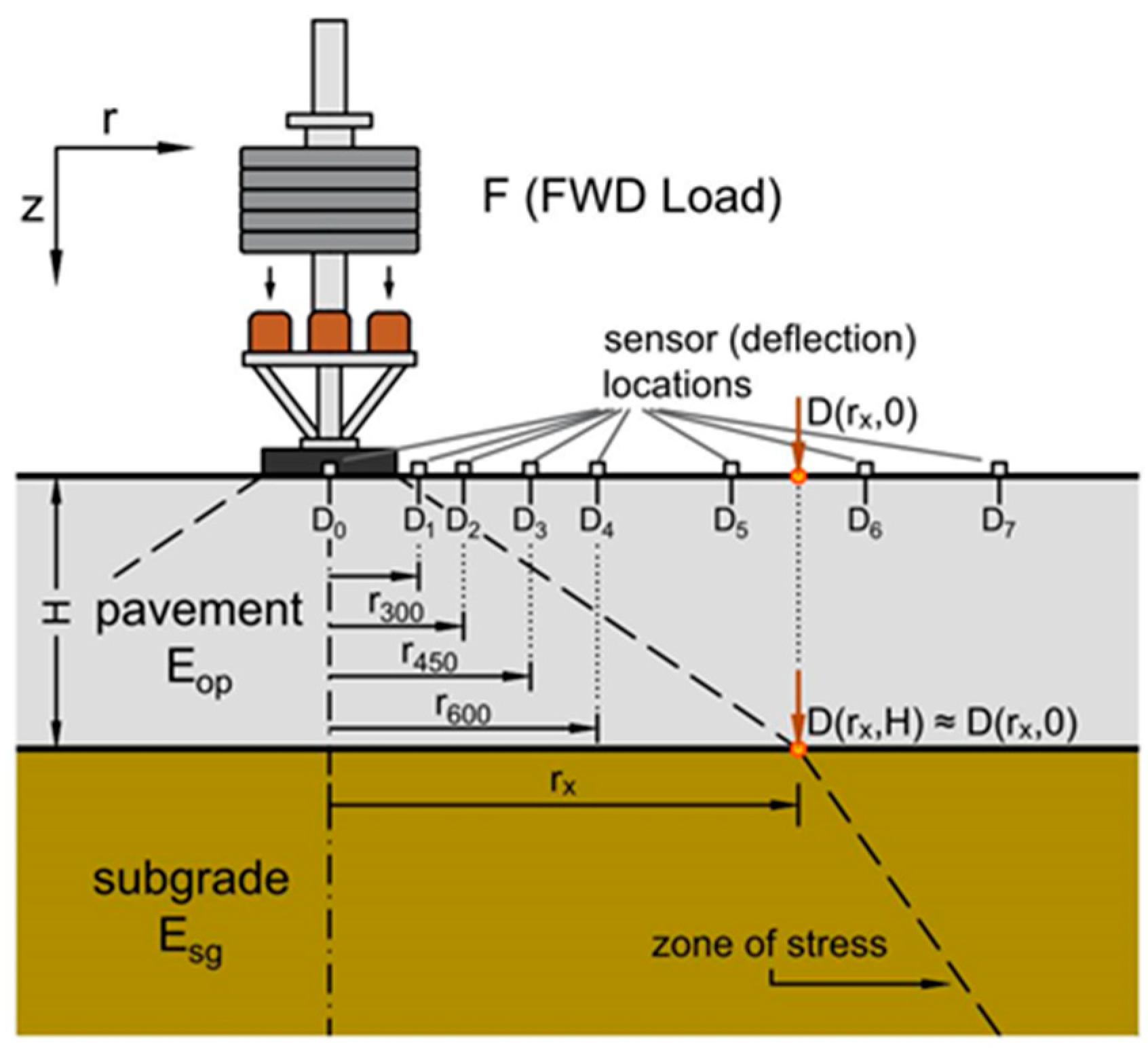
Noureldin developed a simplified method for the direct determination of the road pavement structure layer moduli and layer thicknesses from the FWD measurement results [11,12]. The essence of this method is that on the road pavement surface there is a unique measured point; that is, at $r_x$ radial distance from the load centre, where the $D_x$ deformation is almost exactly equal to the deformation of the subgrade (Figure 4):

$$D_x=D\left(r_x,0\right)\approx D\left(r_x,H\right)$$

(2)

If this unique point is found, then it is possible to back-calculate both the moduli of the subgrade and the pavement structure, as well as to estimate the total thickness of the pavement structure. According to the pavement structure and subgrade deflection data measured by Morgan and Scala at a test section using a modified Benkelman beam (Figure 5), the existence of such a point is rightly supposed [14]. The total thickness of the pavement structure can be calculated using Equation (3), as recommended by [15]:

$$H=0.5{\left[\frac{D_0-D_x}{D_x\left(\frac{r_x}{76.22}-1\right)}\right]}^{1/3}·{\left(4r_x^2-23225.76\right)}^{1/2}$$

(3)

where $D_0$, $D_x$, $r_x,$ and $H$ are defined in mm. Equation (3) is based on the solutions of the two-layered road pavement structures by Burmister and Odemark [16,17], together with the concept of equivalent thickness by Barber [18], as developed by Noureldin and Sharaf [15]. The place of this unique measurement point $r_x$ can be back-calculated itself if trustworthy thickness data are available. 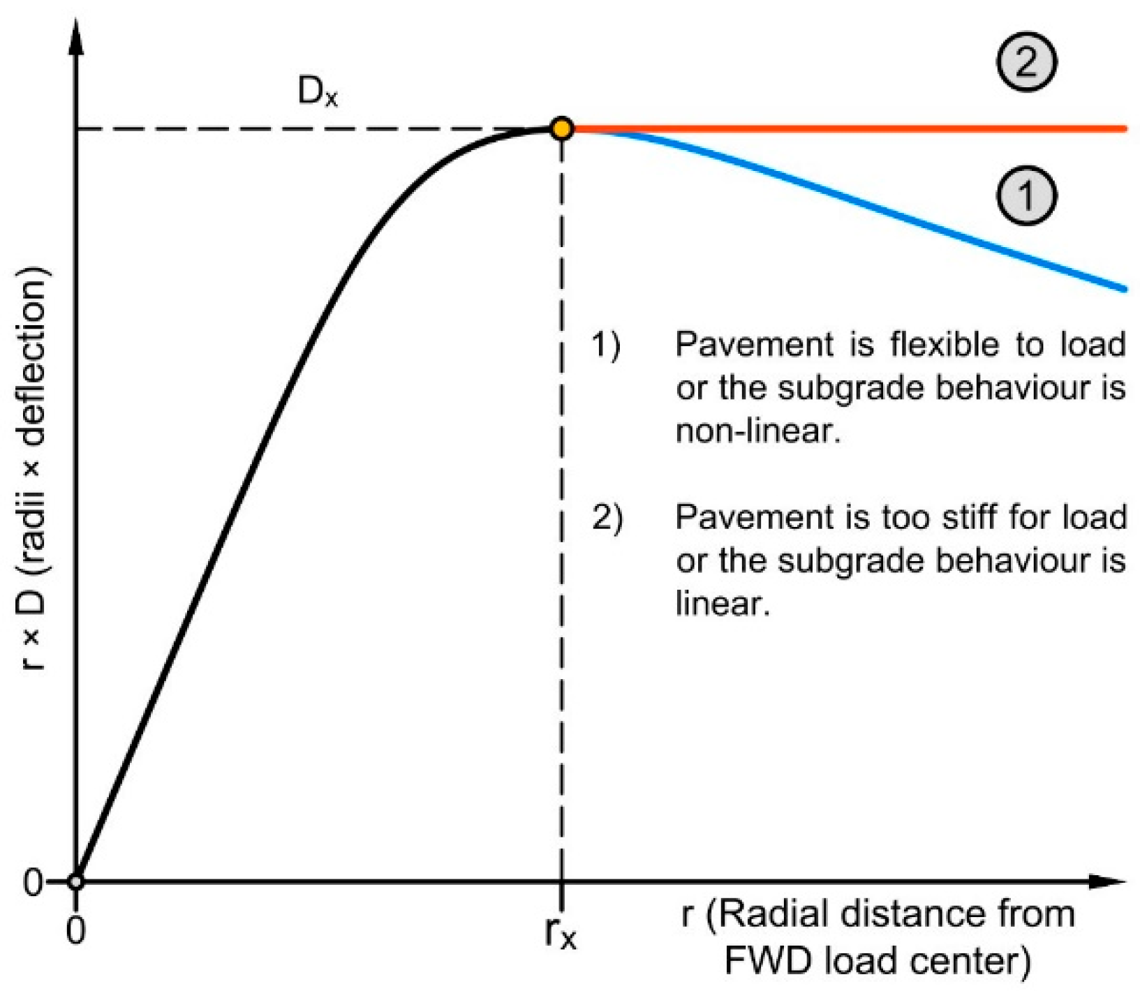All deflection data measured outside the load axle are in correspondence with the $H$ thickness value referring to Equation (3), and from all these scenarios, the adequate case is in accordance with the thickness data of the core sample. For the cases when there are no thickness data, Noureldin’s recommendation is as follows: let us plot a curve of the product of the FWD measurement data $r_x{D}_x$ at $r_x$ radial distances from the load centre, and find the maximum of this curve (Figure 6).

The previously determined $r_x$ distance is substituted into Equation (3). The mathematical background is ensured by the Boussinesq equations for a homogeneous infinite half-space [13]:

$$E_c=2\frac{\left(1-{\mu }^2\right)qa}{D_0}\mathrm{if}r<0.25a$$

(4)

$$E_c=C\frac{\left(1-{\mu }^2\right)q{a}^2}{r_x{D}_x}\mathrm{if}r>0.25a$$

(5)

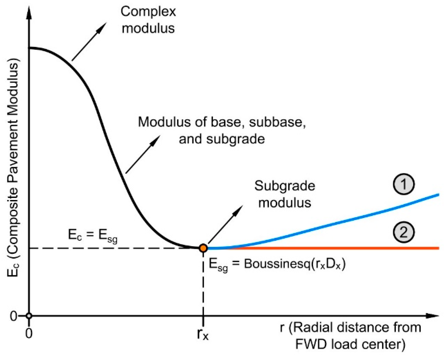
where $E_c$ is the composite modulus, $q$ is the contact stress, $a$ is the load plate radius, $\mu$ is Poisson’s ratio of subgrade, $D_x$ is the measured deflection at $r_x$ radial distance from the load axis, and $C$ is the deformation constant. According to the Boussinesq Equation (5) for a concentrated force, the surface displacement of the homogeneous infinite half-space is inversely proportional to the distance from the load; therefore, the $E_c$ composite modulus has a minimum at the maximum of the product $r_x{D}_x$ (Figure 7). Since the $H$ total layer thickness is defined as from the surface to the lowest layer, and supposing that the bottom subgrade layer has the lowest load-bearing capacity, the composite modulus calculated at $r_x{D}_x$ provides a good approximation:

$$E_{sg}\approx E_c\left(r_x,D_x\right)$$

(6)

In the case where the $r_x{D}_x$ curve has no definite maximum (see type 2 in Figure 6 and Figure 7), the unknown radial distance can be calculated from in-site core samples, GPR sections, or thickness data from a road databank.

The Annex of the AASHTO (1993) Guide contains an algorithm for the determination of the $E_{sg}$ subgrade modulus and the $E_{op}$ equivalent modulus of the total pavement structure. The subgrade modulus is calculated with $a=150$ mm, $q=F/\pi a^2$, and $\mu =0.5,$ applying the Boussinesq Equation (5):

$$E_{sg}=\frac{112.5F}{r_x{D}_x}$$

(7)

A criterium for the $r_x$ value has been established based on the analysis of multi-layer pavement structure models:

$$r_x\ge 0.7a_e$$

(8)

where $a_e$ is the so-called effective radius.

The effective radius is the intersection of the stress cone originating from the loading plate and the subgrade level, which can be approximated by applying Equation (9), based on the equivalent layer thickness theory:

$$a_e=\sqrt{\left[a^2+{\left(H\sqrt[3]{\frac{E_{op}}{E_{sg}}}\right)}^2\right]}$$

(9)

The $E_{op}$ modulus required for the calculation can be back-calculated from the $D_o$ central deflection, the $E_{sg}$ subgrade modulus, and the total $H$ pavement structure thickness by applying Equation (10):

$$D_o=1,5qa\left\{\frac{1}{E_{sg}\sqrt{1+{\left(\frac{H}{a}\sqrt[3]{\frac{E_{op}}{E_{sg}}}\right)}^2}}+\frac{1-\frac{1}{\sqrt{1+{\left(\frac{H}{a}\right)}^2}}}{E_{op}}\right\}$$

(10)

Equations (7)–(10) provide a good basis for the calculation algorithm. Data $r_x$ and $D_x$ from the FWD device are substituted into Equation (7), successively, and the $E_{sg}$ subgrade modulus is calculated for the actual sensor position. After a temperature correction of the $D_o$ load plate centre deflection, using the total $H$ pavement structure thickness and the $E_{sg}$ subgrade modulus, the $E_{op}$ value is calculated by applying Equation (10). The effective radius $a_e$ is calculated by applying Equation (9). The final step is checking the fulfilment of the criterium in Equation (8). If this criterium is fulfilled, the calculation is finished; if not, the process is repeated with the data of the next sector. Despite the AASHTO (1993) procedure not being suitable for a direct back-calculation of the total $H$ pavement structure thickness [19], its presentation is still useful because it provides guidance for the representation and determination of the $r_x$ distance.

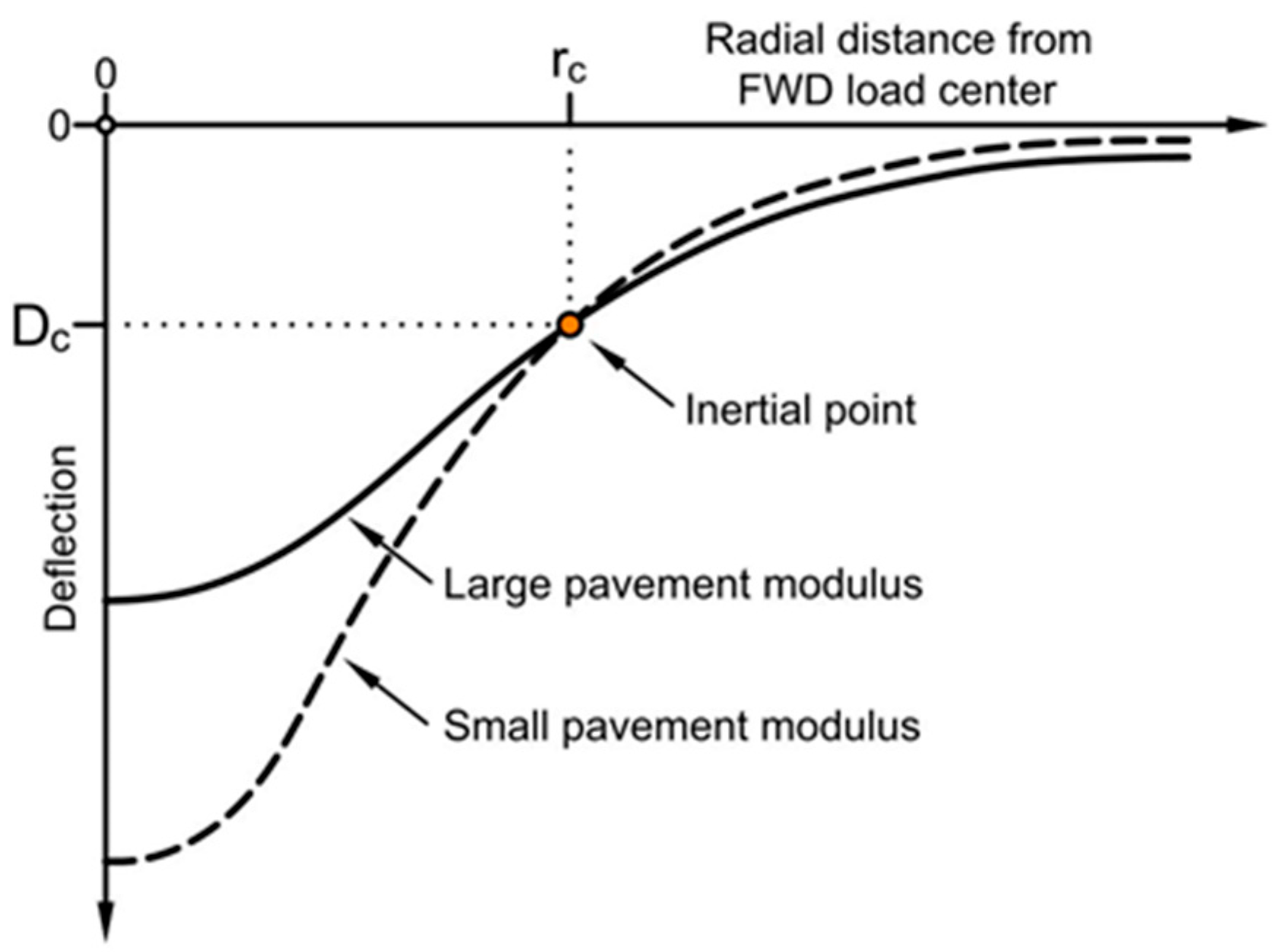
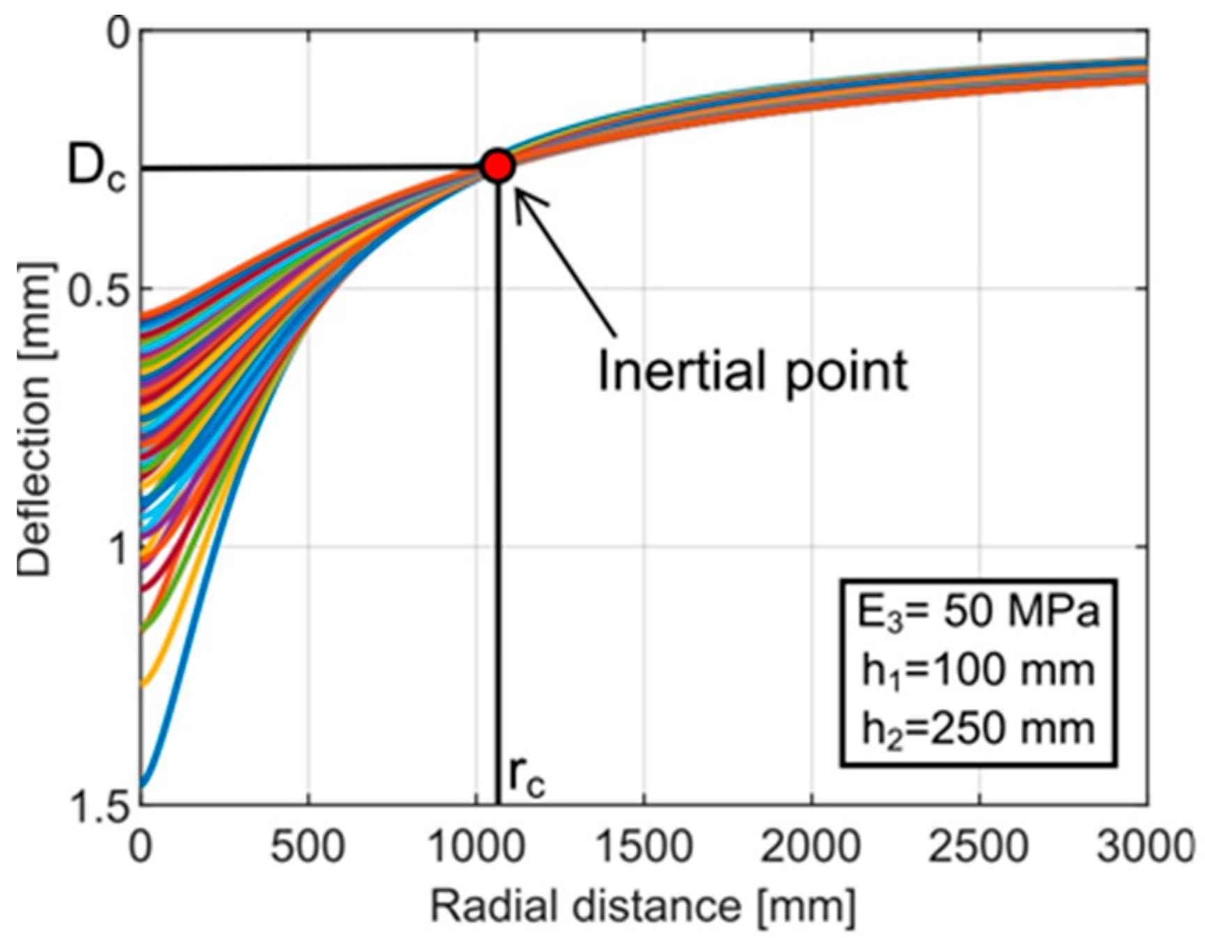
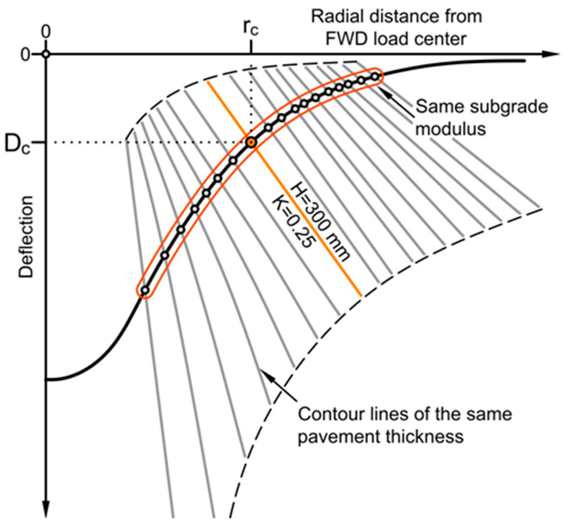
The observations of Noureldin were later verified by Sun and colleagues, who performed the back-calculation of the layer moduli of two-layer concrete pavement structures, discovering that there exists a special point on the deflection bowl, where its deflection value is independent from the modulus of the upper pavement layer [20].

Considering the invariance of this significant point, it has been referred to as the inertial point. This result is based on the calculation of the deflection curve of several two-layer structures. These structures have the same subgrade load-bearing capacity and pavement thickness, only differing in the modulus of the upper pavement layer. It is reasonable to assume that a higher upper pavement layer modulus results in a flattened deflection bowl, while a lesser upper pavement layer modulus results in a steepened deflection bowl on the same subgrade. Moving away from the load axis, an area can thus be identified, where all deflection bowls intersect. 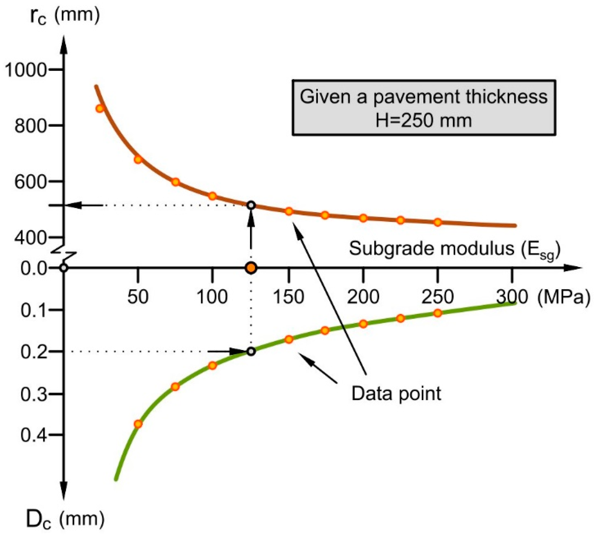Supposing this area is small enough to be approximated as a point, the above-mentioned inertial point is identified (see Figure 8). The radial $r_c$ position of the inertial point and the $D_c$ deflection at this point are correlated with the $E_{sg}$ subgrade modulus and the total $H$ pavement structure thickness (Figure 9):

$$r_c=f\left(H,E_{sg}\right)$$

(11)

$$D_c=f\left(H,E_{sg}\right)$$

(12)

The inertial point has proven to be useful in the back-calculation of layer moduli because a procedure based on the inertial point always provides a definite solution. The method was finally extended for three-layer flexible pavement structures by Zhang and Sun [23,24].

The unique measured point ($r_x$ and $D_x$), introduced by Noureldin and Sharaf, can be equivalent to the inertial point with a good approximation. Hereafter, it is referenced this way:

$$r_x\approx r_c \mathrm{and} D_x\approx D_c$$

(13)

After dealing with the total pavement structure thickness, Noureldin and colleagues made an effort to estimate the total thickness of the upper asphalt layers, developing an empirical formula [12]:

$$h_{AC}=590.24{\left(\frac{D_0-D_{300}}{3D_{300}}\right)}^{1/3}$$

(14)

where $D_0$ is the central deflection, and $D_{300}$ is the displacement of the sensor at 300 mm. Similar results can be found in the work of Plati and colleagues [25], demonstrating a correlation between the $h_{AC}$ total thickness of asphalt layers and the deflection bowl parameters of the FWD device (SCI and BDI indices):

$$h_{AC}=\frac{a+BDI}{b+c·SCI}+\frac{d}{SCI}$$

(15)

where $a$, $b$, $c$, and $d$ are regression parameters. The $h_{AC}=f\left(SCI;BDI\right)$ non-linear function presented in the study suggests that on a given homogeneous road section, from the structural responses acquired by the FWD device, namely deformations, the $h_{AC}$ total asphalt layer thickness can be deduced.

Saltan and Terzi successfully applied neural networks for the back-calculation of layer thicknesses and layer moduli from the measured deflections [26]. Later, Terzi and colleagues tried different data mining techniques in order to determine the upper asphalt pavement thickness from the deflections of the structure. In their studies, the upper pavement thickness varied between 4 and 9 cm in the pavement structure models [27]. The best results have been provided by the KStar (K*) classifier and the neural networks; therefore, these methods are recommended for the assessment of FWD deflections. This idea is supported further by the work of Tarefder and colleagues, where a successful neural network was composed and trained based on FWD device measurement results (max. force, max. displacement, time shift between the force and the displacement, the wave propagation speed at sensors, and the surface temperature), providing a high-accuracy back-calculation of the thickness of both asphalt layers and base layers [28].

In summary, based on recent research, it can be stated that there is a theoretical possibility for the back-calculation of the layer thicknesses of the analysed pavement structure from FWD measurements. The most suitable tool for this purpose seems to be a machine learning method besides the traditional regression analysis.

5. Materials and Methods

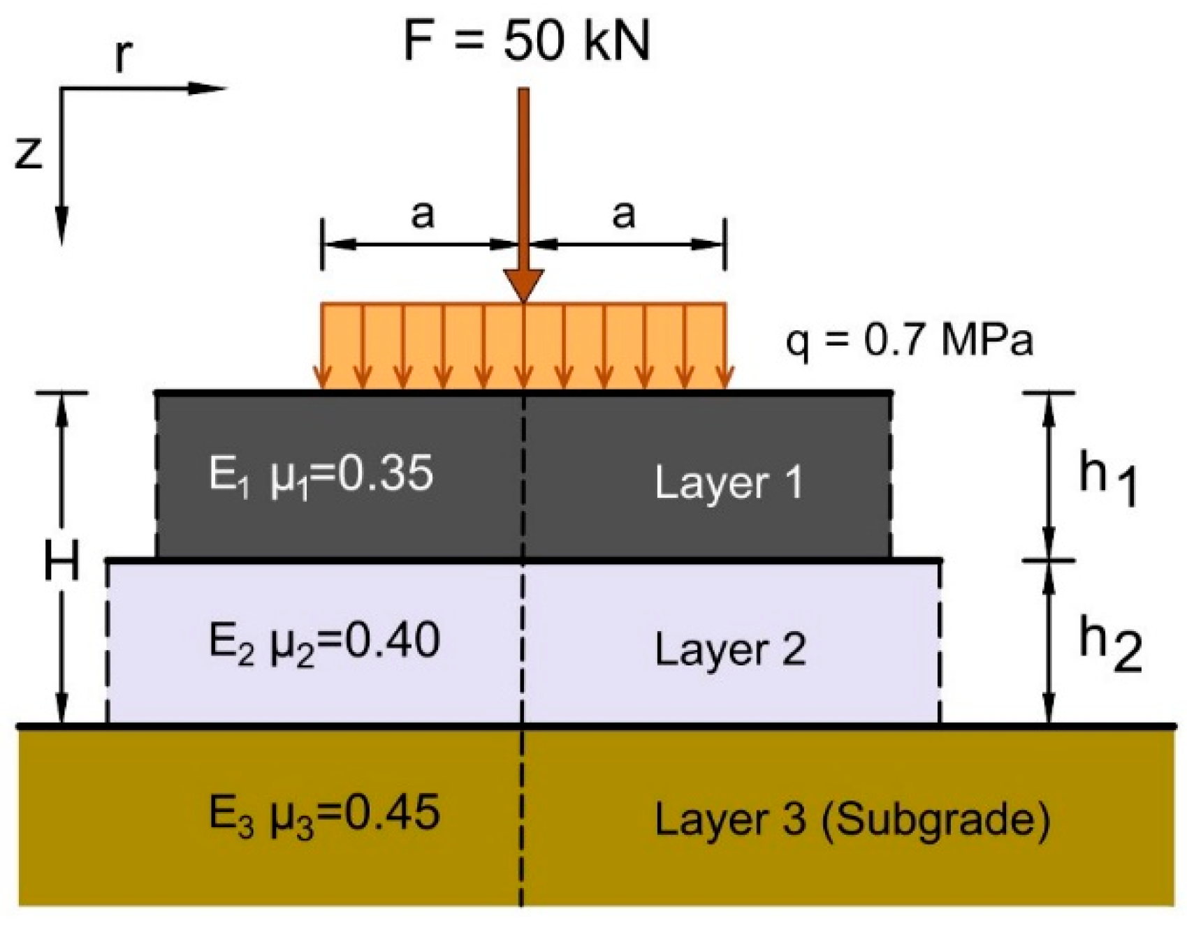
In order to identify inertial points, the first step is the building of a synthetical database of linear elastic three-layer pavement structure models (Figure 10). Every model has a pavement layer of $h_1$ thickness and a base layer of $h_2$ thickness, supported by an infinite elastic half-space. All layer pairs are closely adhesive, and their mechanical behaviour depends only on the Young’s modulus and Poisson’s ratio.

Table 1. Variable parameters of pavement structure used in deflection analysis.

Pavement Parameter	Parameter Range	Increment	Cases
1. layer modulus (E1, MPa)	1000–8000	1000	8
2. layer modulus (E2, MPa)	100–900	100	9
3. layer modulus (E3, MPa)	25–250	25	10
1. layer thickness (h1, mm)	50–250	50	5
2. layer thickness (h2, mm)	100–400	50	7

presents the range of layer thicknesses and material parameters.

In total, 8 × 9 × 10 × 5 × 7 = 25,200 different pavement structures are generated. For the determination of the reactions under a wheel load in the models, a novel software package, the adaptive layered viscoelastic analysis (ALVA), is used, developed by Skar and Andersen for the design and analysis of asphalt pavements in a MATLAB environment [29]. The deflection curve of the pavement is calculated at typical FWD device sensor distances from the load axis: 0, 150, 200, 300, 450, 600, 900, 1200, 1500, and 1800 mm. As the next step, function fitting is performed on the deflections because in the real world there can be a need to extrapolate the FWD device measurement results:

$$D\left(r\right)=\frac{D_{0}4a^2}{{\left(\alpha r\right)}^{\beta }+4a^2}$$

(16)

where $D_0$ is the maximum deflection, $a$ is the load plate radius of FWD, $r$ is the radial distance, and $\alpha$ and $\beta$ are shape parameters [30]. A further analysis is performed using this function for approximating deflections, in order to eliminate any systematic error of later function fitting.

Deflection curves after function fitting are grouped by subgrade load-bearing capacity and layer thicknesses into one of 10 × 5 × 7 = 350 different groups. Every group contains 8 × 9 = 72 pavement structures by the 1- and 2-layer moduli. The plotted deflection curves of structures show their intersection point, that is, the inertial point (Figure 11). In numerical terms, moving from the load axis, a unique radial $r_c$ distance is searched, where the standard deviation of deflections is minimal. The average of the deflections at $r_c$ is equal to the $D_c$ value. An important remark is that because the determination of inertial points is not performed directly from the displacements calculated by the ALVA software, but rather from their approximative function values, these points are better nominated as virtual inertial points, based on the work of Zang [24].

The position of the virtual inertial point can be exactly determined from the deflection data measured by the FWD device, supposing that the $H$ structure thickness is known. In this case, the unknown $E_{sg}$ subgrade modulus is varied until the point with $r_c$ and $D_c$ coordinates is calculated by applying Equations (11) and (12), approaching the deflection curve at a minimum error. Details of this calculation can be found in the work of Zang [24]. In the inverse case, when the $H$ structure thickness is unknown, it is not enough to know the exact value of the $E_{sg}$ subgrade modulus, and a unique solution cannot be obtained because different thickness values belong to every point of the deflection curve. A good demonstration is to plot the FWD data in the system of inertial points.

Figure 12 illustrates that the back-calculation of layer thicknesses can only be performed if the exact position of the inertial point is known.

The Regression Learner App in MATLAB is used to select the best of the various algorithms to train and validate the regression model. Gaussian process regression is chosen to describe the connection between the 350 established virtual inertial points and road pavement structure parameters, being a widespread method in machine learning.

The essence of the method is that the $y=\left\{y_1,\dots ,y_n\right\}$ observations are considered as sample elements of a multi-variable Gaussian distribution. Thinking backwards, a Gaussian process can be assigned to each $f\left(x\right)$ element:

$$f\left(x\right)~GP\left(m\left(x\right),k\left(x,x^{\prime }\right)\right)$$

(17)

The Gaussian process is determined unequivocally by its $m\left(x\right)$ expected value function and $k\left(x,x\prime \right)$ covariance function (sometimes called a kernel function). Details of the exact terminology, development, and application of the Gaussian process regression method can be found in Rasmussen and Williams, as well as in Schulz [31,32]. A detailed presentation of the method is not within the aims of this paper.

After the compilation of a training dataset, the Gaussian process regression model is fitted by the ‘fitgpr’ function of MATLAB version R2021a. The training dataset is based on the 350 virtual inertial points and is regarded as a small-scale dataset; therefore, to avoid overfitting, the $k$-fold cross-validation method is chosen to prove the adequacy of the model. Its essence is that the training dataset is split into $k$ parts, and one ‘fold’ is considered as a validation dataset. The cross-validation ends after $k$ iterations, where each ‘fold’ has been used exactly once as a validation dataset. The model performance is measured by the average of the $k$ results. The advantage of the $k$-fold method is that all elements in the training dataset are used for both training and validation.

Processing the 350 inertial points based on the synthetical database, our experience shows that the $r_c$ and $D_c$ coordinates of the inertial point depend on the $h_1$ and $h_2$ layer thicknesses and their $K=h_1/h_2$ proportions. Consequently, we are not able to prove the observations of Zang and colleagues [24], that the behaviour of a three-layer system can be well approximated by a two-layer model, where the upper unified $H$ pavement thickness is equal to the sum of $h_1$ and $h_2$. This is demonstrated by the calculation examples in

Table 2. Example of the effect of the pavement layer thickness ratio on the inertial point.

Esg (MPa)	h1 (mm)	h2 (mm)	rc (mm)	Dc (mm)	K (-)	H (mm)
50	100	200	980	0.2886	0.50	300
50	200	100	1186	0.2450	2.00	300
50	150	250	1277	0.2227	0.60	400
50	250	150	1568	0.1889	1.67	400

. The results show that the position of the inertial point depends on not only the $E_{sg}$ subgrade modulus and the total $H$ layer thickness, but also the $K$ thickness proportion of the layers.

Henceforth, the connection between virtual inertial points and pavement structure characteristics can be determined by the Gaussian process regression in Equation (18):

$$H=GP\left(r_c,D_c,K,E_{sg}\right)$$

(18)

For the validation of the Gaussian process regression model, the dataset is split into 5 parts. Applying the MATLAB software, the parameters and characteristics of the Gaussian process regression model are determined, as summarised in

Table 3. Hyperparameters of the Gaussian process regression model.

Optimised Hyperparameters	Training Results
Basis function: Linear	RMSE (Validation): 1.876
Kernel function: Nonisotropic Rational Quadratic	R-Squared (Validation): 1.00
Kernel scale: 2.174	MSE (Validation): 3.5192
Signal standard deviation: 86.7265	MAE (Validation): 1.0127
Sigma: 0.00010219	Prediction speed: ~21,000 obs/s
Standardise: true	Training time: 132.93 s

.

The algorithm for the deflection-based layer thickness calculation is compiled by applying the Gaussian process regression model. The main steps of the algorithm are as follows:

Step 1.

Determination of the position of the inertial point ($r_c,D_c$) from the deflection bowl. The inertial point is where the composite modulus reaches the minimum, as shown in Figure 7. If there is no unique maximum on the $r$ vs. $rD$ plane (Figure 6), then the position of the inertial point is estimated by the analysis of core samples.

Step 2.

Substitution of the coordinates of the inertial point into Equation (5) for the calculation of the $E_{sg}$ subgrade modulus.

Step 3.

Determination of the $K$ proportion of layer thicknesses according to the road plan or core samples.

Step 4.

Estimation of the total $H$ pavement thickness applying the GPR model.

Step 5.

Calculation of the $h_1$ and $h_2$ layer thicknesses based on the total $H$ pavement structure thickness and the $K$ proportion: $h_1=KH/\left(K+1\right)$ and $h_2=H/\left(K+1\right)$.

To verify our calculations, the results are compared with the results of the procedure in the AASHTO (1993) Guide Annex. Finally, starting from the FWD deflection measurement data, in terms of the knowledge of layer thicknesses, layer moduli are determined by applying the BAKFAA (Computer Program for Back-calculation of Airport Pavement Properties) software.

The developed assessment procedure was tested on an experimental road section in Hungary, on the western bypass of Gyöngyös city, approximately 85 km from Budapest. On the experimental road section, two non-destructive methods, the FWD and the GPR, were applied for surveying road condition parameters. The spatial arrangement of measurements is shown in Figure 13. A subjective condition assessment and a video recording were also performed on the experimental road section.

The positions of reflexion cracking, surface distress, and engineering structures were determined (Figure 14) in order to take these features into account during the evaluation of the GPR sectional results.

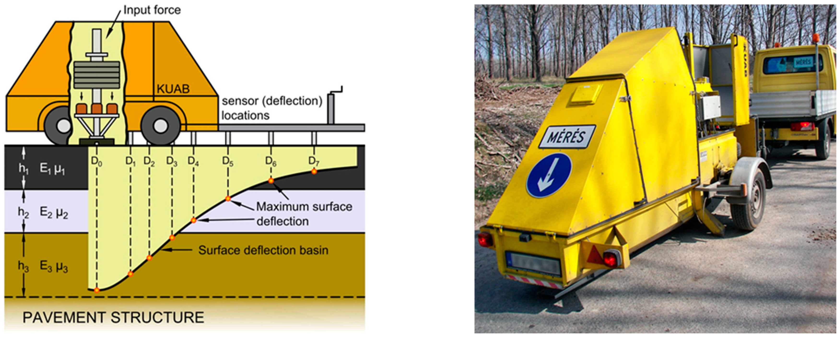
The KUAB-type FWD device (Figure 1) has a load plate radius of 150 mm, and the distances of the seven sensors from the load axis are: $r_0=0$, $r_1=200$, $r_2=300$, $r_3=450$, $r_4=600$, $r_5=900$, and $r_6=1200$ mm. The KUAB device stores $D_0$, $D_1$, $D_2$, $D_3$, $D_4$, $D_5$, and $D_6$ deflections at sensor positions as a reaction of the 50 kN load force. In the middle of the lane of the surveyed section, every 25 m, two drops were performed: a pre-loading and a measurement. At each point beside the deflection data, the load force was recorded, as well as the air and pavement temperatures. All deflection data were afterwards corrected to a 50 kN load.

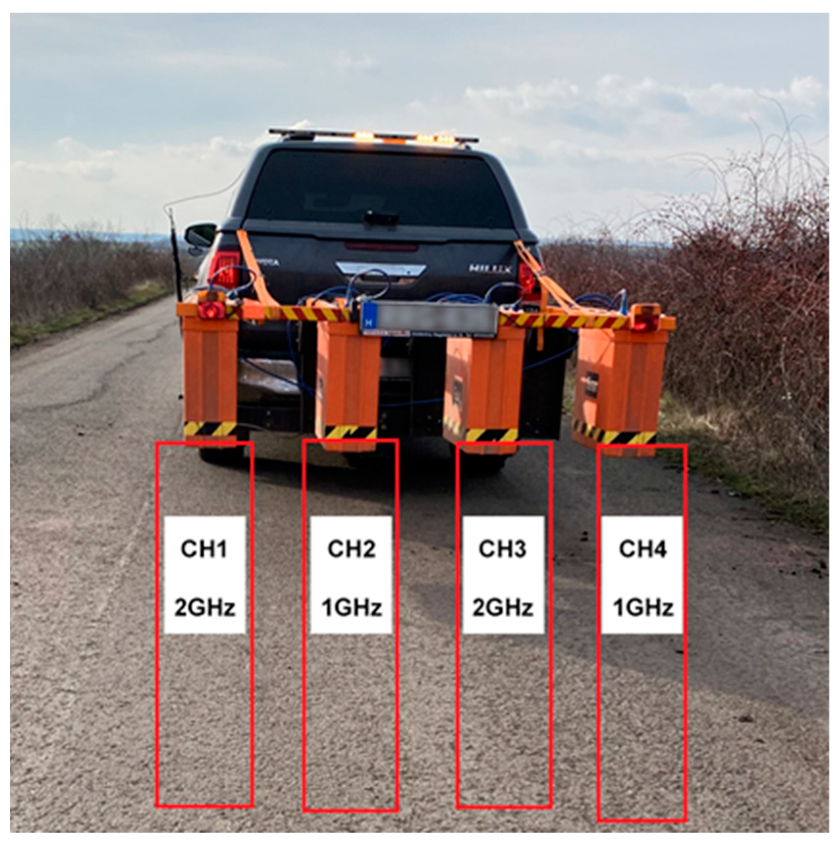
The georadar device for the survey was provided by the RODEN Engineering Office, Hungary (Figure 15). The GSSI-type 1 GHz and 2 GHz frequency air-connected antennas are situated behind the measurement car at 1.5 m, above the pavement surface at approximately 250 mm. The position of the antennas is shown in Figure 15. The survey was performed at 16 km/h speed and 50 scan/m. The raw data were recorded by a high-speed multi-channel SIR-30 data recorder and controller system. In the present paper, only the results of the 2 GHz antennas are processed and evaluated by applying the RADAN software.

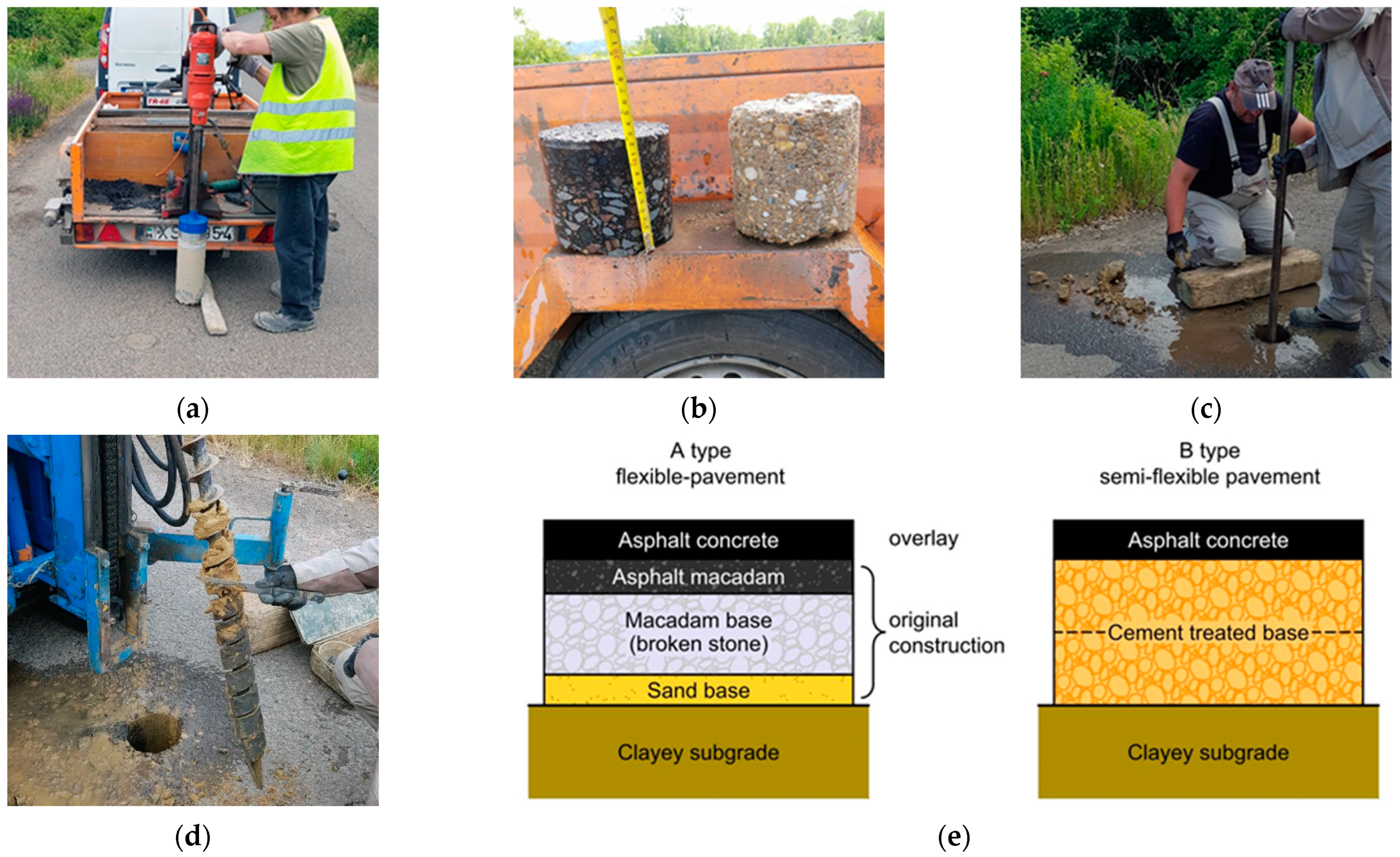
For comparison, the layer order of the surveyed road section was determined by using destructive methods every 100 m (Figure 16). The core sampling technology proved useful for the determination of the exact layer thicknesses of asphalt layers and hydraulic bonded layers. In the case of the old granular coarse crushed stone base, a manual breakthrough was necessary. The subgrade sampling was performed by continuous spiral drilling, using the established core sampling holes.

Two main pavement structure types are identified from the measurements. The first (type A) is a flexible road pavement structure originating from an asphalt macadam. The subgrade is a bond clayey soil; therefore, the crushed stone road base was laid on a sand layer to equalise the difference in thickness. Another bitumen sprayed–crushed stone layer of 5–7 cm was laid on the load-bearing sub-base. Later, after the deterioration of the structure, a new asphalt concrete-strengthening layer was constructed. The second (type B) is a semi-rigid structure laid on a cement-treated granular road base, in some cases consisting of two layers; further asphalt layers were constructed on that base layer.

6. Results and Discussion

Concerning non-destructive survey methods, the assessment of the GPR results indicates a considerable difference between the structure of the left and right lanes. A feasible cause is that in the past decades, the road section has sometimes been reconstructed, lanes have been widened using various technologies, the vertical alignment has been corrected, and the pavement structure itself has been strengthened. Based on the radar sectioning, the right lane consists of two different parts (Figure 17). According to core samples, the first part is a crushed stone base of the macadam type, between 1000 and 1542 m, and the second part has a hydraulic (CTB) road base between 1542 and 2000 m. The exact location of the structural change was acquired from GPR data, while the layer materials in the structure were determined from core samples.

Figure 17 shows the GPR-measured layer thicknesses and those from the core samples. All GPR sections show clear layer boundaries; however, in the macadam base part, in some cases, the lower layer boundaries are not always determinable. Since the permittivity of the asphalt-wearing course and binder course is similar, the boundary between these two layers cannot be determined. Consequently, for the analysis, only the total asphalt thickness was applied. The average difference in the asphalt thickness estimated from the GPR results compared with the core samples is 5.59 % on the first part, and only 1.63 % on the second part. The higher inaccuracy in the first part is caused by the lower asphalt macadam layer of varying thickness, and its assessment cannot be performed more accurately based only on the GPR measurements. The radar section of the second part indicates that the hydraulic (CTB) road base was constructed in two layers. The core samples indicate the same; moreover, the sample was sheared at the layer boundary and sometimes teared. This way, only the upper hydraulic layer thickness can be compared with the GPR measurement results. The average difference in the hydraulic layer thicknesses is 4.34% compared with the core samples.

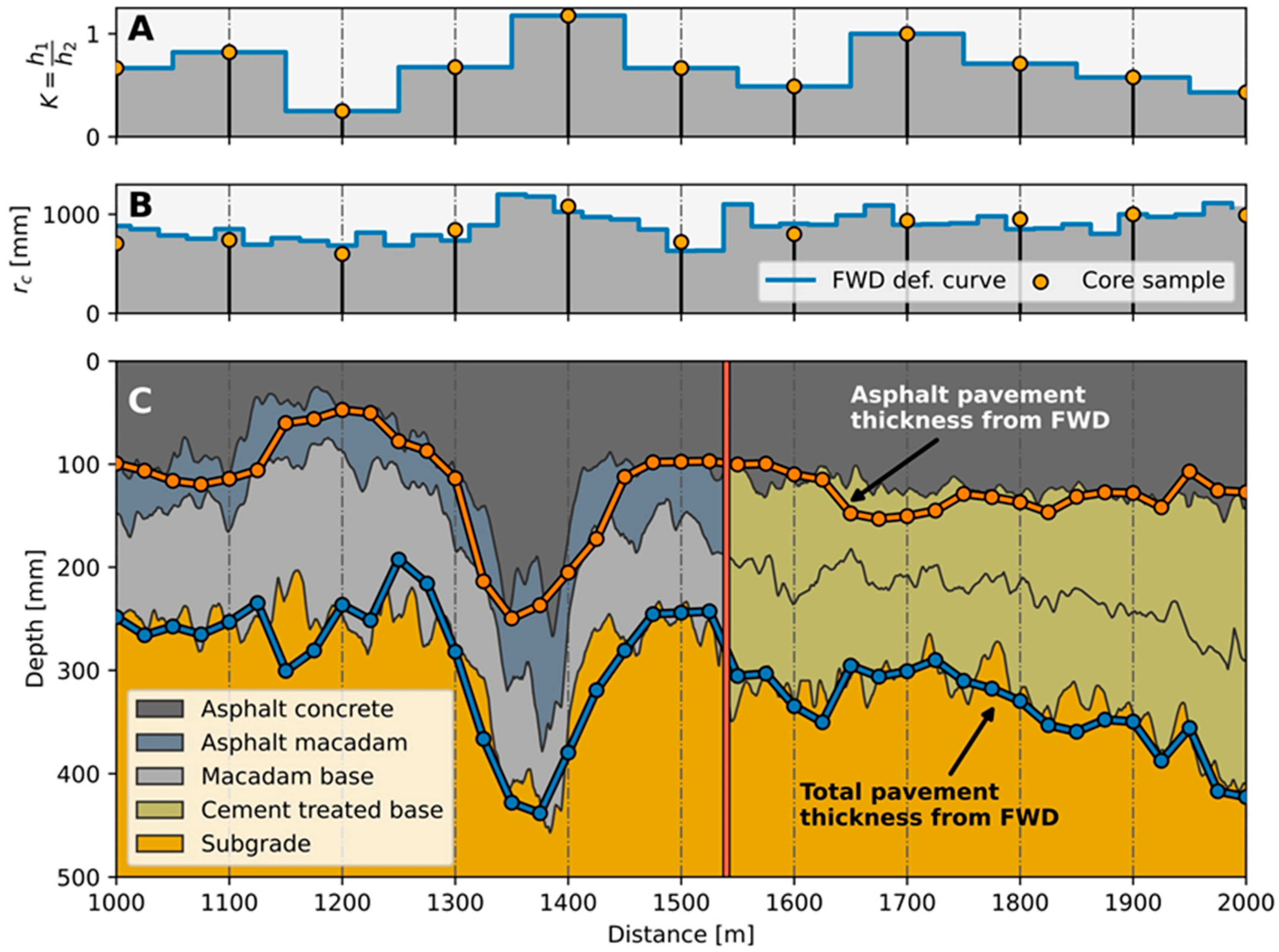
The $K$ layer thickness proportions were determined from the pavement structure core samples, extrapolated by a stepwise function (Figure 18A). An $r_c$ value was estimated for each drop position from the deflections measured by the FWD device (Figure 18B). The $r_c$ radial distances deducted from the deflection bowl were calibrated by thickness data from core samples. The $D_c$ deflections belonging to the final $r_c$ distances were calculated by applying Equation (16). Substituting $r_c$ and $D_c$ data pairs into Equation (5), the $E_{sg}$ subgrade modulus was determined. This way, all data were available for the Gaussian process regression model. An estimate of the total $H$ pavement structure thickness was performed, substituting the required data into the $GP\left(r_c,D_c,K,E_{sg}\right)$ model. As a final step, using the $K$ layer thickness proportion, the total $H$ pavement structure thickness was split into the $h_1$ asphalt layer and $h_2$ base layer thicknesses (Figure 18C).

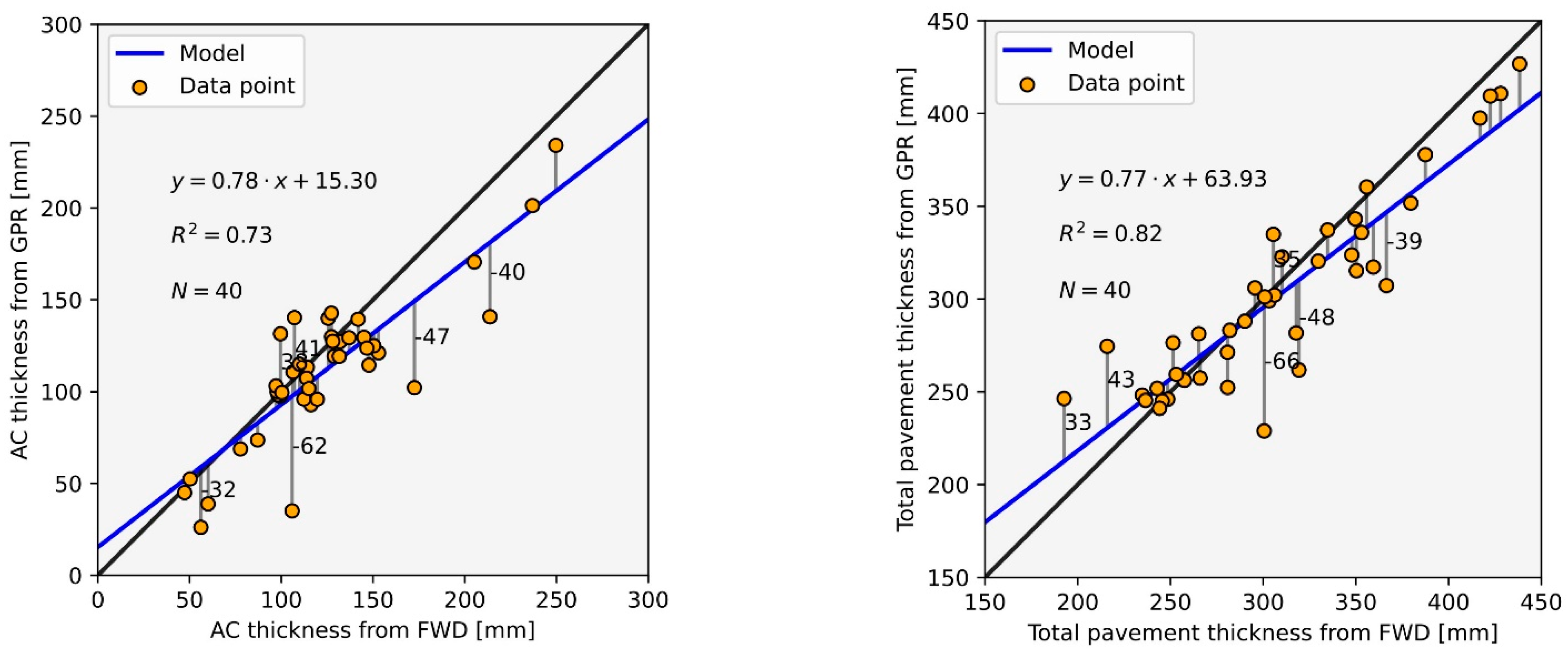
Figure 18C indicates that there is a good correlation between the layer thicknesses measured by the GPR device and calculated from the FWD deflections. Figure 19 contains a direct comparison of layer thicknesses determined from the GPR and FWD measurement results. GPR data were chosen for the verification of the predicted thicknesses because many more measured points were available compared with the core samples. The total pavement thickness determined by the GPR cannot be taken as absolutely accurate because in some cases the crushed stone base and the subgrade material cannot be distinguished. The fact that the comparison of total pavement structure thickness estimated from the FWD survey and measured by the GPR produces a line close to the 1:1 slope can be considered as a noteworthy result in and of itself. Total asphalt thickness shows a larger deviation from ideal circumstances; one cause of this may be the use of the $K$ layer thickness proportion for estimation. There may be some error because of the spatial extrapolation of the proportion of $K$ layer thickness based on the core samples. The average difference between the two survey methods is ±45 mm, which is acceptable for practical calculations.

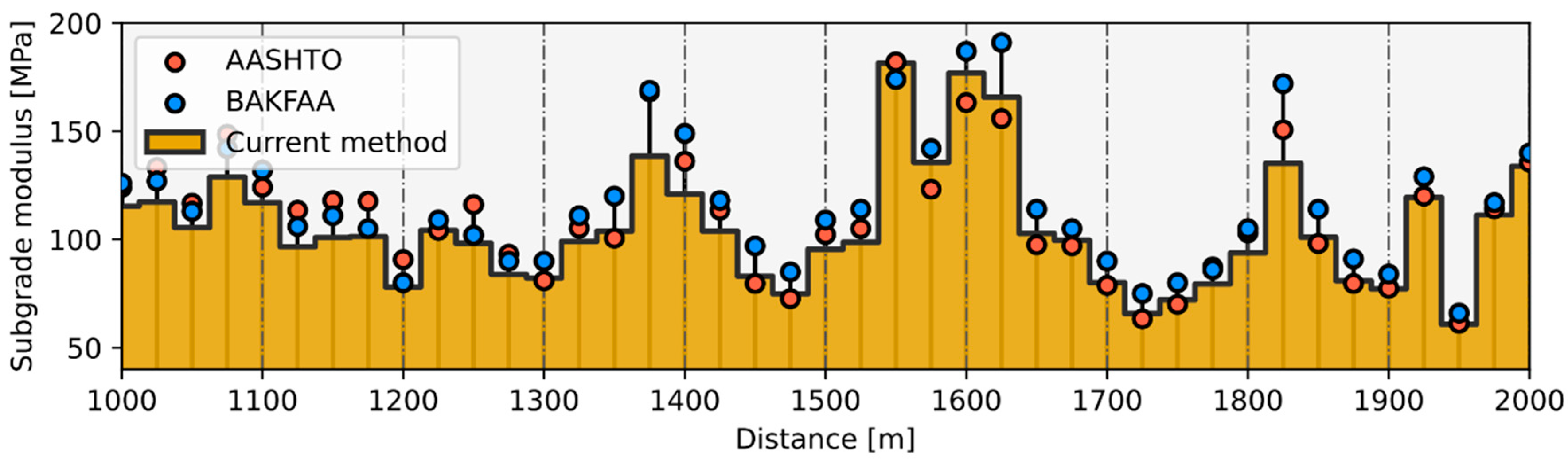
The $E_{sg}$ subgrade moduli calculated by the inertial point method were compared with the results of the AASHTO (1993) procedure and the results of the BAKFAA software. In the graphical plot of these results, given in Figure 20, it can be observed that the subgrade modulus based on the inertial point provides a good approximation of the results of the two other methods. Our currently developed method characteristically estimates modulus values that are 5–10 MPa less than those of the other two methods.

Based on core samples between 1000 m and 1542 m, the first flexible road section (with a macadam base) has an average load-bearing capacity of 100 MPa. Next is a short section with a hydraulic base between 1542 m and 1625 m, which has a higher average load-bearing capacity of 165 MPa. This outlying value can be explained because there is a bridge structure between 1590 m and 1600 m. The experimental road section is connected to this bridge on a high embankment, which is better protected from adverse water movements. The remaining part of the second section has an average load-bearing capacity of 95 MPa. The relatively high load-bearing capacity values can be explained by the very hard clay subsoil.

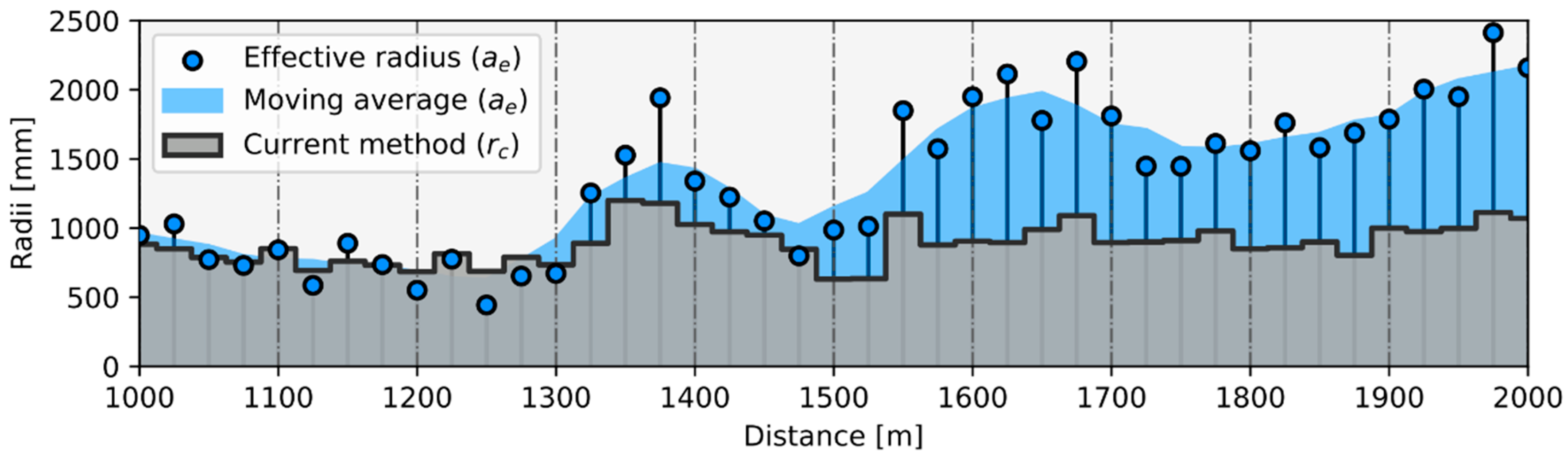
The subgrade load-bearing capacity results show that Boussinesq’s Equation (5) is valid for a homogeneous infinite half-space, which is not sensitive to the exact value of $r_x$. A more expressive demonstration can be made by comparing the $r_c$ distances of inertial points to the $a_e$ effective radius used in the AASHTO (1993) procedure. Plotting data onto a longitudinal section, it can be observed that on the section with a flexible crushed stone base, the $r_c$ distances roughly meet the effective radius values (Figure 21). The assumption that the $r_c$ is approximately equal to the effective radius is therefore true in the case of flexible structures. On the contrary, on the semi-rigid second section with a hydraulic road base, the two values differ significantly.

The cause of the difference is that the value of $a_e$ is influenced by the $E_{op}$ modulus of the road pavement structure above the subgrade, and its effect is stronger on the second section of higher load-bearing capacity. The inertial point, in turn, is not dependent on the $E_{op}$ modulus of the upper road pavement structure; therefore, its value remains roughly constant even in the case of a semi-rigid structure.

The $r_c$ radius of the inertial point varied between $4.5a$ and $7.5a$, being positioned at an average of $6a$ distance from the load axis. This means that the subgrade modulus is characterised well by the deflection value of the sensor at $6·150 \mathrm{mm}$, i.e., $900 \mathrm{mm}$ from the load axis. A more interesting result is that on the 1000 m experimental road section, the stress cone originating from the loading plate was registered as 20° ± 2°, against the value of 34° frequently cited in the literature [33,34].

Despite this research work being in its initial phase, the presented results can be considered as valuable. The inertial point method provides a rather accurate estimation for not only the subgrade modulus but also the total pavement structure thickness. The robustness of the method shall be verified in the future by FWD measurements performed in different seasons, before recommending its practical utilisation. This is a possible direction for future research.

7. Summary

This paper presents a method for the back-calculation of layer thicknesses based on the deflection data acquired by a non-destructive FWD device. FWD and GPR devices are often not available together; therefore, this research is of practical significance. The developed method is based on the inertial point principle and provides not only the total pavement structure thickness, but also the total asphalt thickness, at each FWD drop point. Nevertheless, the proposed method is not fully non-destructive because core sampling is required to determine the $K$-layer thickness proportion and layer materials. Besides thicknesses, the subgrade modulus can also be back-calculated at a high accuracy, using the inertial point. Based on the assessed data of the experimental section, the $r_c$ radius value of the inertial point is not sensitive to the stiffness of the layers of the pavement structure, depending only on the total pavement structure thickness and the subgrade modulus. For verification, our calculations have been compared with the subgrade modulus results of the AASHTO (1993) procedure, obtaining similar results. The procedure’s effective radius value ($a_e$) is close to the $r_c$ radius value in the case of flexible pavement structures but differs significantly in the case of semi-rigid structures. Moreover, the presented method is suitable for tracing seasonal changes in the load-bearing capacity of the subgrade, beyond the back-calculation of layer thicknesses. Further research should aim to find a more exact determination of the $r_c$ radius value of the inertial point because this is a key issue for the utilisation of the method. By solving this problem, the layer thicknesses can be determined from the data of continuous deflection measurement devices, such as the Curviameter or the Rolling Wheel Deflectometer. Comparing the results of the two non-destructive survey methods, the uncertainties in data representation can be eliminated, providing better and more exact road pavement structure diagnostics.