Article

Multi-Response Optimization of Surface Grinding Process Parameters of AISI 4140 Alloy Steel Using Response Surface Methodology and Desirability Function under Dry and Wet Conditions

1
Department of Industrial and Production Engineering, Jashore University of Science and Technology, Jashore 7408, Bangladesh
2
Department of Industrial and Production Engineering, Bangladesh University of Textile, Dhaka 1208, Bangladesh
3
Department of Industrial and Production Engineering, Bangladesh University of Engineering and Technology, Dhaka 1000, Bangladesh
4
Department of Chemical Engineering, COMSATS University Islamabad, Lahore 54000, Pakistan
5
Department of Nanotechnology and Advanced Materials Engineering, Sejong University, Seoul 05006, Korea
*
Authors to whom correspondence should be addressed.
Coatings 2022, 12(1), 104; https://doi.org/10.3390/coatings12010104
Submission received: 30 November 2021 / Revised: 4 January 2022 / Accepted: 7 January 2022 / Published: 17 January 2022
(This article belongs to the Special Issue Recent Advances in Bioactive Film Coatings)

Abstract

:
The effect of four controllable input process parameters of AISI 4140 steel, cross-feed, workpiece velocity, wheel velocity, and the depth of cut were experimentally investigated under dry and wet conditions. Three responses, contact temperature, material removal rate (MRR), and machining cost during surface grinding of AISI 4140 steel, were considered. The process was optimized using a recently developed combined methodology based on response surface methodology (RSM) and desirability functional approach (DFA). RSM generated the models of the responses for prediction while DFA solved these multi-response optimization problems. The DFA approach employed an objective function known as the desirability function, which converts an estimated response into a scale-free value known as desirability. The optimum parameter was attained at the maximum overall desirability. An analysis of variance (ANOVA) was conducted to confirm the model adequacy. From the results of the study, for equal weights of responses, the corresponding optimal values of the input parameters cross-feed, workpiece velocity, the wheel or cutting velocity and the depth of cut were found to be 6 mm/pass, 12 m/min, 15 m/s, and 0.095 mm respectively in wet conditions. The corresponding predicted output responses were: 134.55 °C for the temperature, and 7.366 BDT (Taka, Currency of Bangladesh) for the total cost with an overall desirability of 0.844. Confirmation testing of optimized parameters, i.e., checking the validity of optimal set of predicted responses with the real experimental run were conducted, and it was found that the experimental value for temperature and total cost were 140.854 °C and 8.36 BDT, respectively, with an overall desirability of 0.863. Errors of the predicted value from the experimental value for equal weightage scheme were 4.47% for the temperature and 7.37% for the total cost. It was also found that if the temperature was prioritized, then the wet condition dominated the overall desirability, which was expected. However, if the cost was given high weightage, dry condition achieved the highest overall desirability. This can be attributed to the cutting in the wet condition which was more expensive due to the application of cutting fluid. The proposed model was found to be new and highly flexible in the sense that there was always an option at hand to focus on a particular response if needed.

Graphical Abstract

1. Introduction

Grinding is widely used as an ultimate machining process in manufacturing of components incorporating excellent geometric accuracy and satisfactory surface finish. Compared with other machining processes, such as turning and milling, grinding process generates a substantial amount of heat at the grinding zone (almost 10–30 times of that in turning) due to the very high energy input per unit volume of material removal raising the temperature of the grinding zone [1,2]. Excessive temperature may cause thermal damage to the workpiece such as workpiece burn, phase transformations, undesirable residual tensile stresses, cracks, reduced fatigue strength, and thermal distortion and inaccuracies [3]. It may also cause premature failure of the cutting tools, rapid oxidation, and corrosion [4,5]. The most commonly used dry grinding has the advantages of cost-effectiveness and environment friendly nature with no pollution despite having major drawbacks namely thermal damage, high friction, high residual stress, and high wheel-wear [6]. On the other hand, wet cutting condition removes heat from the cutting zone. However, it does not always seem to be effective as it consumes a large amount (i.e., 8 L/min) of coolant which is not economically feasible and has a significant impact on the ecology and internal environment (workshop) [7,8]. Hence, a trade-off among material removal rate (MRR), cutting zone temperature, and machining cost is needed for effective machining.
The magnitude of residual stresses caused by grinding is determined by the physical and mechanical characteristics of the grinding material as well as the parameters, such as wheel speed, workpiece speed, depth of cut, grinding wheel composition, and lubrication. These, in turn, determine the temperature gradient in the grinding zone [9]. In steels, an empirical connection between peak residual tensile stress and maximum grinding zone temperature has been identified [10].
Investigating cutting zone temperature and heat transfer in grinding requires specific temperature measurements. Thermal imaging, optical fiber, foil/workpiece (single pole) thermocouple, and embedded (double-pole) thermocouple are some prominent temperature measuring techniques. Because of its relative simplicity, low cost, precision, and dependability, the integrated thermocouple technique is the most commonly utilized. A two pole thermocouple was welded to the bottom of a blind hole drilled close to the ground surface from the underside of the workpiece using this approach [11,12]. Changfeng Yao et al. investigated the impact of wheel speed and depth of cut on the temperature of Aermet 100 steel during surface grinding using three different types of wheels. As a temperature measurement device, they employed a single alumina wheel, a white alumina wheel, and a CBN wheel with coolant. A thermocouple was also used. They discovered that the overall heat flow of a single alumina wheel is the greatest, which is due to two factors: high tangential grinding force and poor thermal properties of the grinding wheel [13].
The response surface methodology (RSM) is a collection of mathematical and statistical approaches that may be used to model and analyze issues in which a response of interest is influenced by multiple factors and the goal is to maximize this response [14]. Bhushan used the response surface method and desirability analysis to examine the impact of cutting parameters during the turning of 7075 Al alloy SiC composite in order to minimize machine power consumption and enhance tool life [15]. Using RSM technique, Rudrapati et al. investigated the influence of cylindrical grinding process parameters on responses such as workpiece vibration and surface roughness [16]. A multi-objective genetic algorithm was used to optimize process parameters for the required results, and the projected model was validated using a confirmatory test. M. Janardhan and A. Gopala Krishna used response surface methodology (RSM) to determine the optimum machining parameters leading to minimum surface roughness and maximum metal removal rate in surface grinding process operation on EN24 steel [17]. Aravindand Periyasamy optimized process parameters by using the Taguchi method and response surface methodology (RSM) for surface grinding of AISI 1035 steel and they considered grinding wheel abrasive grain size, depth of cut, and feed as process parameters and Surface roughness as output response [18].Venkatesan et al. focused on the comparative performance of input parameters viz. speed, feed, and depth of cut on cutting force, roughness, tool wear, and chip morphology of dry and MQL machining conditions on Nimonic 90 alloy with the aid of RSM [19]. Manohar et al. optimized output responses viz. surface roughness, cutting forces, and MRR as a function of input process parameters, viz. cutting speed, feed rate, and depth of cut with RSM and desirability function approach (DFA) while turning Inconel 718 using coated carbide tools [20]. Naresh et al. focused on the optimization of process parameters namely, cutting speed, feed rate, and depth of cut which influence the output response surface roughness and material removal rate with grey relational analysis (GRA) and desirability function analysis (DFA) in CNC milling of AISI 304 stainless steel [21]. Buranska et al. demonstrated multi-criterial optimization with desirability function analysis (DFA) of input factors cutting environment, feed for two defined target functions roughness, and cylindricity for drilling of aluminum alloys [22]. Borchers et al. investigated different manufacturing processes of AISI 4140 steel with regard to surface modification but not identified the optimum machining parameters [23]. However, unfortunately, very little literature is available on process parameter optimization of surface grinding with DFA. A comprehensive summary from previous literature on grinding type, the material used, optimized input parameters, and output responses along with the optimization (analysis) techniques of surface grinding is presented in Table 1.
It is apparent from the literature that the process parameters such as cross-feed, workpiece velocity, wheel velocity, and the depth of cut have a significant influence on the temperature, MRR, and production cost in the grinding process for different cutting conditions. The temperature in turn affects the finishing of the workpiece and tool life. To the best of the authors’ knowledge, no study has been conducted on the surface grinding of AISI 4140 steel to evaluate, compare, and optimize contact temperature, MRR, and machining cost in dry and wet machining conditions so far. Again, the combined methodology of RSM and DFA in optimization of machining parameter is rarely found in this relevant field. Combined approach of RSM and DFA known as desirability optimization methodology (DOM) is efficient in determining the optimum antagonist responses (here temperature and MRR) which are led by different input machining parameter.
This study looks into the grindability of AISI 4140, a chromium-molybdenum alloy steel. The chromium component allows for effective hardness penetration, while the molybdenum element guarantees consistent hardness and strength. Carbon steel is alloyed with one or more alloying elements such as manganese, silicon, nickel, titanium, copper, chromium, and aluminum to create alloy steels. These metals are added to provide characteristics not seen in standard carbon steel. Superior toughness, ductility, and wear resistance under quenched and tempered conditions are among the desired characteristics of AISI 4140 [23]. Hence it has a lot of applications in the engineering field.
Thus, in this research work, we optimize contact temperature, MRR, and machining cost during surface grinding of AISI 4140 steel using a combined methodology based on surface methodology (RSM) and desirability functional approach (DFA). From the literature study presented above and in the Table 1, it can be said that the optimization of surface grinding process parameters of AISI 4140 steel using a combined methodology based on surface methodology (RSM) and desirability functional approach (DFA) for both wet and dry condition is rarely studied. Thus, the novelty of this work is to study the multi-objective optimization with response surface methodology (RSM) and desirability functional approach (DFA) of surface grinding of AISI 4140 steel. Therefore, the contribution of this research can be outlined as follows:
  • Experimentally investigation the influence of the input machining parameters (cross-feed, workpiece velocity, wheel velocity, and the depth of cut) on three responses (contact temperature, material removal rate (MRR), and machining cost) during surface grinding of AISI 4140 steel.
  • Establishment of an empirical equation of each output responses in terms of input parameters based on the experimental data. Further this mathematical model is used to predict the output responses.
  • Optimization of the output responses (minimum contact temperature, maximum MRR, and minimum machining cost) based on the DFA methodology. Further, optimal set of input parameters are investigated for these optimal responses.
Finally, DFA aids to find out optimal set of input parameters along with their corresponding output responses such as contact temperature, MRR, and machining cost. In addition, DFA further optimizes the input process parameters to get the minimum contact temperature, maximum MRR, and minimum machining cost.

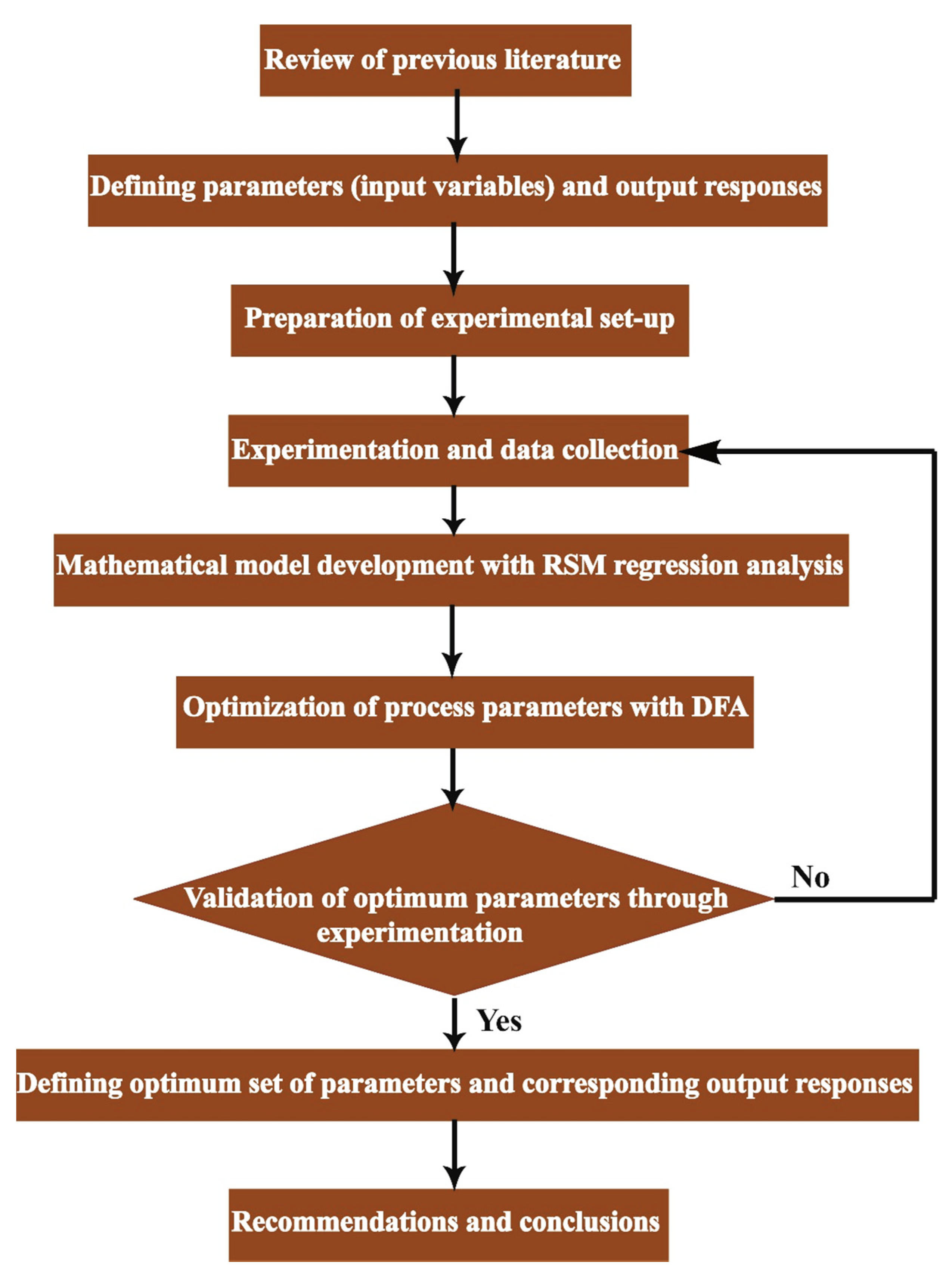
2. Methodology and Experimental Procedures

The materials and methods have been described with sufficient details to allow others to replicate and build on the published results.
In this study, RSM and DFA have been anticipated as solution methodology. The outline of this research is summarized in Figure 1. Materials and instruments, experimental setup, RSM, and DFA methods are detailed in the subsequent subsections.

2.1. Materials and Instruments

Workpiece: The surface grinding operation is performed on AISI 4140 alloy steel (Bozhong Metal Group, Shanghai, China). It is a chromium-molybdenum alloy steel. The chemical composition, dimension, and other physical properties of the workpiece material are listed in Table 2.
Grinding wheel: Grinding wheel is the basic cutting tool in grinding operation. The grinding wheel used in this experiment was alumina oxide vitrified, i.e., glassy and noncrystalline, from NORTON (Shanghai, China). Its dimension is 14 in × 1.5 in × 3 in. This grinding wheel (FE 38A100L5V) is used in accordance with the machining circumstances and manufacture’s exhortations. According to the standard system of grinding wheel markings, the specifications of the grinding wheel are: type of abrasive: aluminum oxide; grit size or the grain size: 100 µm, i.e., fine; grade: L, indicating medium, i.e., neither soft nor hard; the porosity or the dense to open: 5; and the type of bonding: V, i.e., vitrified. A Single point diamond, HS050 (Shanghai Sanxin Diamond Tools Co., Ltd., Shanghai, China) dresser was used to dress the grinding wheel. A total depth of dressing 40 µm was achieved.
Cutting fluid: This experiment was carried out both in dry and wet conditions. Castrol Syntilo 9954 (Shangai, China) was selected as cutting fluid in wet machining conditions. An emulsion was made on this synthetic coolant basis with concentration of 5%. Its density is 1066 kg/m3. Single nozzle open metal-tube type was used to apply coolant at a flow rate 5 L/min. Flow rate was measured with Z-5615 Panel Flowmeter (Emerson Electric Limited, Rayong, Thailand).
Thermocouple and Digital Multimeter: A system composed of a K-type thermocouple and a digital multimeter were employed to determine the contact temperature between the grinding wheel and the workpiece.

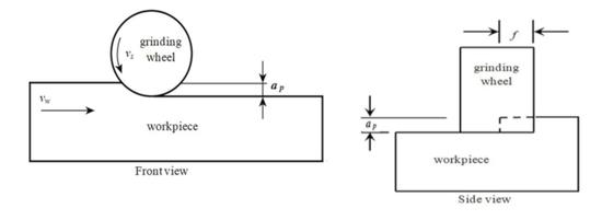
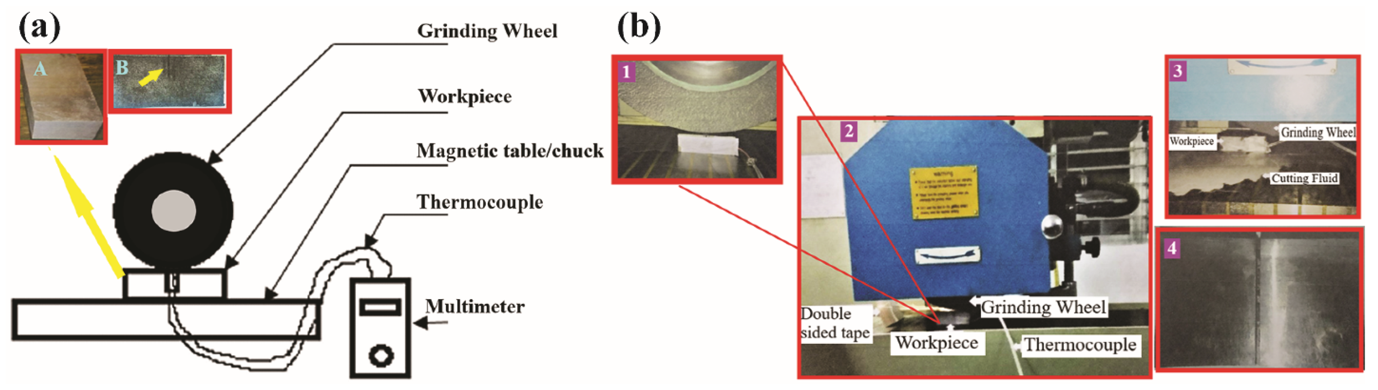
2.2.1. Experimental Set Up

The grinding machine used in this experiment was an Okamoto (Woodlands Newtown, Singapore) hydraulic surface grinder (Model: PSG-125) with a driving power of main motor 10 HP. It was a column type surface grinding machine and originated in Japan. The optimal position of the nozzle during flood cooling was such that the jet became tangent to the wheel and impinged on the contact region between the workpiece and grinding wheel. To achieve this, the nozzle was placed at a 15° angle with the ground and at a 35 mm distance, which was kept constant. For better accuracy, prior to each experimental run the grinding wheel was dressed with a single-point diamond dresser with a total depth of dressing 40 µm along with a peripheral wheel speed of 15 m/s and feed rate of 400 mm/min, respectively. Each experimental run was conducted twice to check the consistency of the result. The grinding condition, presented in Table 3, incorporated specifications of grinding conditions along with dressing cut parameters.
The input parameters with their respective levels are shown in Table 4. Here, grinding wheel speed was set at 15–25 m/s which is analogous to some of the previous values found in the literature. Khan et al. set the cutting speed at 15–35 m/s to optimize output responses for grinding of AISI D2 steel [43]. Gholami and Azizi set the wheel speed at 1963–2749 m/min (32–45 m/s) for grinding of 1.2080 steel while optimizing time, cost, and surface roughness [28]. Rabiei et al. set the wheel speed at 30 m/s for 100Cr6 hardened steel to improve the performance of the MQL technique [41]. Singh et al. put the wheel speed at 22 m/s to optimize the output responses at different lubricating methods in the surface grinding of ‘Ti-6Al-4V-ELI’ [38]. Input parameters, such as workpiece velocity, wheel velocity, cross-feed, and cutting condition, have two levels each (Figure 2a), while depth of cut has five levels. The multilevel full factorial design (24 × 5 = 80) was applied to run 80 experiments for this research work. Figure 2b shows the multilevel full factorial design of the design of experiments (DOE) applied to conduct experiments. Detailed calculations of the DOE are presented in the Supplementary Materials.
For this surface grinding operation, a temporary setup is arranged to determine the contact temperature between the grinding wheel and the workpiece. This system is composed of a K-type thermocouple and a digital multi-meter connected systematically. The schematic diagram of the experimental setup is depicted in Figure 2a.
Close to the cutting zone, EMF (electromotive force) is generated at the thermocouple junction which is determined from the multi-meter at the other pole of the thermocouple. The embedded thermocouple was inserted into the material to measure the temperature. For this insertion, a very small slot was created by matching thermocouple dimensions. The smaller the size of the slot for positioning thermocouple, the more accurate the data as it minimized the transmission of disturbance to the local temperature field. Hence, a slot of 0.5 mm width and 8 mm depth was made by the EDM (Electrical Discharge Machining) wire cut machine (Figure 3a) on the workpiece and the thermocouples’ junction was installed into the slot to make sure that it remains very close to the contact region of grinding wheel and workpiece (Figure 3b). Hence this method enabled a direct temperature measurement of the workpiece surface. Thermocouple junction into the slot was insulated to minimize convection and radiation heat transfer. The other junction of the thermocouple, which had positive and negative terminals, was connected with the corresponding points of the digital multi-meter. The thermocouple measured the EMF generated due to the presence of the temperature gradient during machining which was transmitted through the thermocouple and displayed at the digital multi-meter. This EMF was converted to the temperature using the following equation to get the elevated temperature at the contact zone of the grinding wheel and the workpiece:
θ ( ) = 75.28 + 63.05 v ( mV ) 0.57 v 2 ( mV )
Cutting zone temperature in terms of digital multi-meter EMF reading was obtained by varying the cutting parameters, including spindle speed, feed, and depth of cut for different cutting conditions (dry condition (Figure 3b) and wet condition (Figure 3b)). To calculate MRR, material removed after each pass of machining per minute for a particular set of input parameters was determined. This action was carried out through slide calipers which measured the reduction of height of the workpiece after each round of machining. This reduction of height was multiplied with the length and width of the workpiece to obtain the total amount of material removed. A stopwatch was used to determine the time for each round of machining. Total amount of material removed was divided by total machining time for each round to get experimental MRR. Total cost included utility (power consumption), labor, and cutting fluid cost for this research work. To calculate utility cost, power consumption for each round of machining was determined, which was further multiplied with cost per unit of consumption. Labor and cutting fluid costs were obtained by multiplying the machining time for each round with cost per unit time. For each set of input parameters, output responses were measured thrice, and their geometric means were used for further mathematical analysis. The measurement procedure was a continuous procedure and measured at a single set up. For each set of input parameters, a particular round of machining was performed (each rounds repeated thrice) and these rounds were performed sequentially for all sets of input parameters. Each round was followed by the measurement of responses. Response surface methodology (RSM) and desirability function approach (DFA) were used as the statistical methods to process the experimental results. Under this arrangement, surface grinding operation was conducted in a horizontal surface grinding machine. The machined surface of the workpiece looks like that shown in Figure 3b after the operation.
To optimize the surface grinding process, response surface methodology (RSM) and desirability function approach (DFA) were employed in the solution methodology. Response surface methodology and desirability function approach are detailed in the subsequent sub-sections.

2.2.2. Material Removal Rate (MRR) Calculation

The amount of material removed per unit time (theoretically) from the workpiece by machining is determined by the following equation [20]:
M R R = 100 × v w × a p × b
where:
  • MRR is the material removal rate (mm3/min)
  • vw is the workpiece velocity or longitudinal table travel velocity (m/min)
  • ap is the depth of cut (mm)
  • b is the width of the cut (mm).

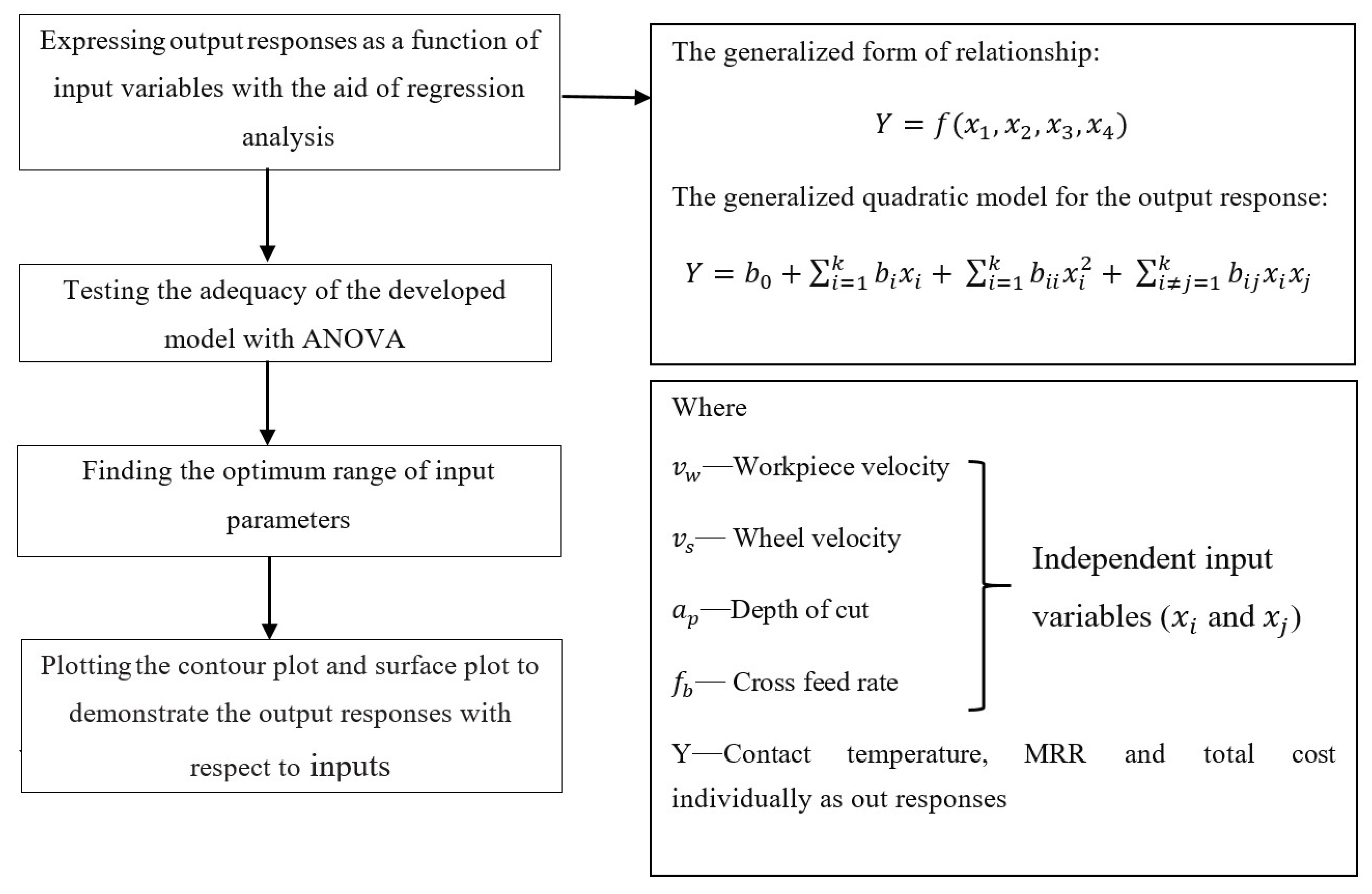
2.2.3. Response Surface Methodology

Design of experiments is most commonly adopted to investigate the impact of input variables on the output responses at various fields including machining parameter optimization. An optimal set of input variables can be found systematically with fewer trials, effort, and time by this process. Response surface methodology (RSM) is one of the most popular methods among the design of experimental methods. RSM is an empirical model developing method with mathematical and statistical analysis (especially regression analysis) to optimize an output response (dependent variable) which is regulated by several input parameters (independent variables). A comprehensive outline of RSM methodology is depicted in Figure 4. Coefficients of the generalized quadratic model (b0, bi, bii, and bij) were calculated, based on the least-squares method [44].
RSM models mathematically how two or more independent parameters regulate the output response of a process or system and also find the optimal set of independent parameters. With the aid of ANOVA significant parameters (which influence the output response) are screened out from the non-significant parameters [45,46,47].

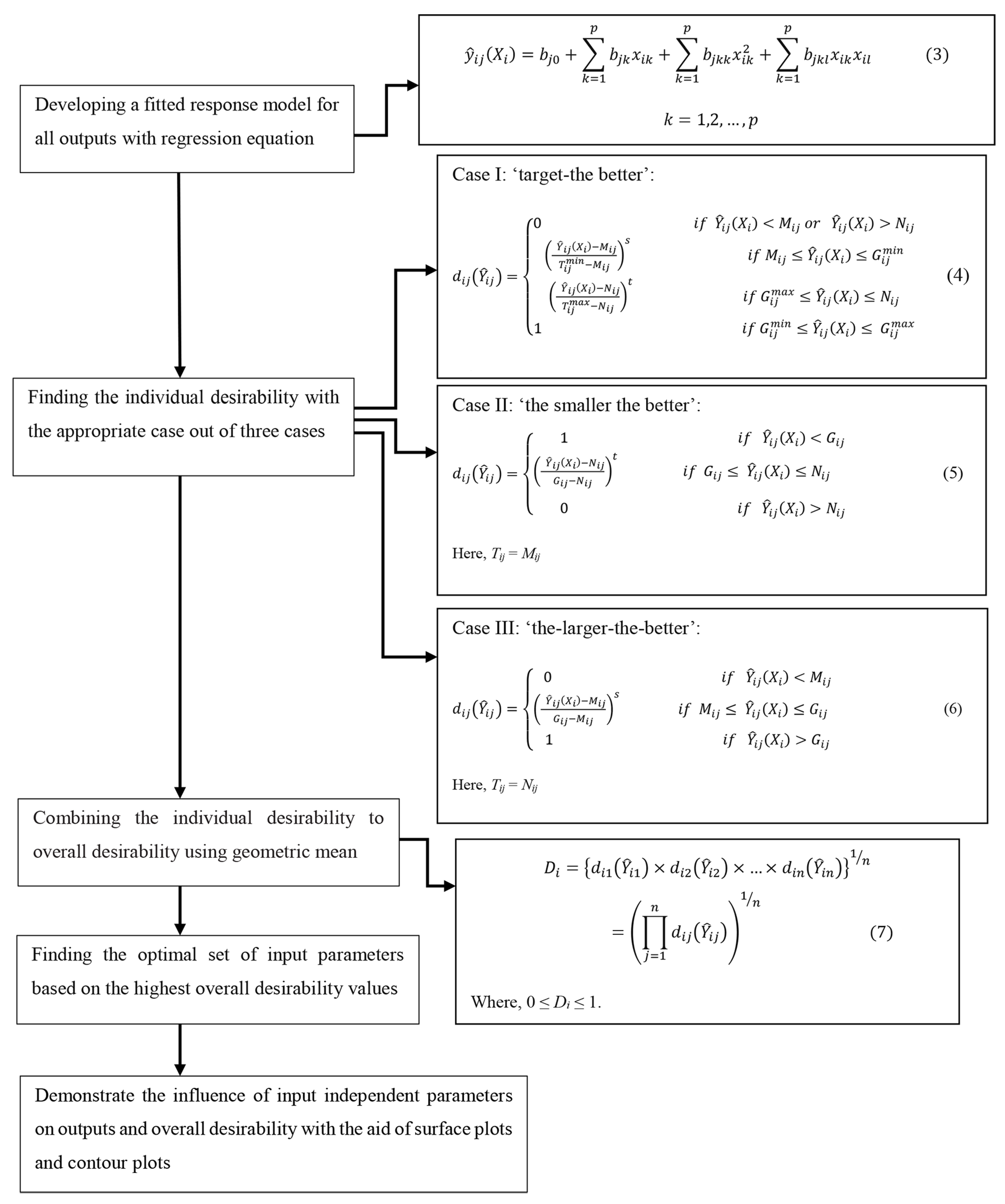
2.2.4. Desirability Function Approach

RSM focuses on the optimization where there is only one output response. However, in the actual scenario of process optimization, there is more than one output response of interest, and these responses may be contradictory. In this case, to determine the optimum set of input parameters, all the output responses should be taken under consideration at the same time. This scenario is termed as a multi-response problem or multi-response optimization (MRO) problem [48]. In this study optimization of contact temperature, MRR, and machining cost are the key objectives, but these output responses have a conflicting interest as contact temperature and machining cost need to be minimized while MRR needs to be maximized. Since multiple conflicting objectives are present, this is termed as a multi-response optimization (MRO) problem. So far, to solve MRO problems numerous methods have been developed, i.e., desirability function approach [49,50] and loss function approach [51].
Among the MRO techniques, DFA is very simple to implement and easy-to-understand approach for the industry practitioners. The underlying principle of DFA is to convert a multi-objective problem into a single objective problem with the aid of mathematical conversions. Derringer and Suich (1980) demonstrated a multiple objective problem with the help of desirability-function to make it popular for industry practitioners for optimizing the multiple quality characteristic problems [52]. DFA deals with an objective function, named desirability function, and converts the calculated output from the desirability function into a scale-free value called desirability with one out of three cases. In this work a multi response optimization with DFA was used and the equations showed in the DFA flowchart (Figure 5) are reported by Manohar et al. and the steps are illustrated as flowchart in Figure 5 [20].
X i k = ( x i 1 , x i 2 , x i 3 , x i 4 ) = ( v s i , v w i , d i , f b i )
where:
  • Xi—input variables value for i in the experiment, I = 1, 2,…, m.

3. Results and Discussions

The main focuses of this study were solving the multi-response optimization problem in surface grinding of AISI 4140 alloy steel with the aim of maximizing the desirability function. Three responses, temperature, material removal rate (MRR), and total machining cost, were to be optimized with respect to cross-feed, workpiece velocity, the wheel or cutting velocity, and the depth of cut under dry and wet conditions. It can be found that the wheel velocity and the workpiece velocity of this study are analogous to the input parameters of the study reported by Sadeghi et al. [53]. However, they used a depth of cut which was lower than that in our study due to the use of AISI 4140 hardened steel instead of regular AISI 4140 steel (used in our study). Sadeghi et al. studied the advantages of MQL technique through the evaluation of grinding forces and surface quality for grinding AISI 4140 hardened steel. They set the input parameters wheel speed at 30 m/s, work speed at 10, 20, 30, and 40 m/min, depth of cut at 0.005, 0.010, and 0.015 mm [53]. Response surface methodology (RSM) was applied to model the responses for prediction whereas the desirability function approach (DFA) was employed to resolve the multi-objective optimization problem. The use of DFA also enabled the assignment of numerous weights to the responses according to their relative importance. Analysis of variance (ANOVA) was conducted to confirm the model adequacy. For equal weights of responses, the optimal values were found to be 6 mm/pass of cross-feed, 12 m/min of workpiece velocity, 15 m/s of the wheel or cutting velocity, 0.095 mm of the depth of cut in wet condition, and a maximum overall desirability value of 0.863. Additional results were obtained for the unequal weights of response variables. Surface and contour plots were also developed for further examination of the obtained result. The estimated equation for total cost and temperature by RSM under different environments (dry and wet) is given below:
Temp dry = 977.242 + 7.25 × f b 3.36 × v w + 2.375 × v s 21602.5 × a p + 145538 × a p 2 0.212 × f b × v w 0.071 × f b × v s 28.223 × f b × a p 0.0042 × v w × v s + 23.7174 × v w × a p 8.89 × v s × a p
Cos t dry = 9.4224 0.978 × f b 0.49943 × v w + 0.0043143 × v s 22.83 × a p + 97.1215 × a p 2 + 0.0534 × f b × v w 0.00007 × f b × v s + 1.434 × f b × a p + 0.000157143 × v w × v s + 0.1429 × v w × a p 0.01552 × v s × a p
Temp wet = 423.585 + 4.63 E 14 × f b 0.4011 × v w 1.44345 × v s 7958.2 × a p + 52175.4 × a p 2 2.78 E 16 × f b × v w 3.11 E 16 × f b × v s 4.36 E 13 × f b × a p 0.0137251 × v w × v s 7.89962 × v w × a p + 23.8998 × v s × a p
Cos t wet = 39.7315 5.84 × f b 3.1523 × v w + 0.2445 × v s + 344.873 × a p 1587.53 × a p 2 + 0.354143 × f b × v w + 0.01057 × f b × v s 5.1552 × f b × a p 0.01133 × v w × v s + 0.1195 × v w × a p 2.25172 × v s × a p
From the equations, it is obvious that the temperature and the total cost were affected by the depth of cut more significantly than any other input parameters, as the coefficient of the depth of cut was much higher than any other coefficients in the equation. In the RSM, each estimated equation was developed considering values of 40 sets of input variables. Afterward, these equations were used to predict the responses. It was found that the predicted and experimental values are quite proximate. The mean error for temperature and the total cost was less than 2% and 5%, respectively. This depicts that the experiments were conducted in the right way and uncertainty in input parameters was lower. After that, response surfaces for each combination of input parameters were constructed, as shown in Figure 5 and Figure 6. For the dry condition (Figure 6a), the optimum levels for workpiece velocity, wheel velocity, depth of cut, and cross-feed were 12–20 m/min, 2–10 m/s, 0.065–0.085 mm, and 0.1–2.5 mm/pass, respectively, to minimize the temperature. For the wet condition (Figure 6b), the optimum levels for workpiece velocity, wheel velocity, and depth of cut were 15–20 m/min, 1–12 m/s, and 0.062–0.080 mm, respectively, to minimize the temperature. However, cross-feed had no significant effect on temperature in wet the condition. Similarly, the response of total cost was analyzed in this way and optimum levels were determined from contour plots (Figure 7). The results are represented in Table 5.
To carry out the experiments, target values for all independent variables (input parameters) and three dependent variables (response) were selected. The optimization criteria for these two sets of variables are presented in Table 6. Target values for the independent variables should lie within the range of the parameter settings that were used to conduct the experiments. The input parameter’s range for optimization was determined based on the optimum range of input parameters derived from RSM contour plot and from previous literature. Luu Anh Tung et al. set table speed (m/min) at four levels [6,8,10,12] to investigate its influence on surface roughness of grinding 9CrSi tool steel [50]. Kruszynski and Lajmert set cross-feed (mm) at three levels [2,4,8] to maximize MRR during grinding of 34CrAl6C steel [51]. Again, depth of cut (mm) and wheel speed (m/min) were set at three levels (0.06, 0.08, 0.1) and (1963, 2356, 2749), respectively, for time, cost, and surface roughness optimization during 1.2080 steel grinding by Mohammad Hadi Gholami and Mahmood Reza Azizi [52]. Besides, for optimum production cost, production rate and surface finish the wheel speed (m/min) were 2000 and 1998, respectively, by quadratic programming and genetic algorithm for rough grinding, and 2000 and 1986, respectively, by quadratic programming and genetic algorithm for finish grinding at a surface grinding operation by Saravanan et al. [53]. The wheel velocity from literature and that we have considered are quite analogous, as it is in m/min units in the literature, but we used the unit m/s. Since the cutting condition is a categorical variable (i.e., either dry or wet), it does not have any lower or upper bound. Among the dependent variables, the target for temperature should be to minimize it since the higher temperature has an increasingly adverse effect on the surface finish and other material characteristics of the workpiece. Total cost, which includes utility cost, labor cost, and cutting fluid cost, should also be minimized. The MRR should be maximized because higher MRR results in the lower unit production cost of the produce. The lower and higher levels of these variables were set to the minimum and maximum values that were observed in the experiment. Alternatively, one can use more relaxed or stringent bounds. Regardless, the overall outcome of DFA should remain the same.
The individual desirability values were calculated according to Equations (4)–(6) with DFA as depicted at Figure 5. The individual desirability values were calculated for each experimental run. The overall desirability value was then the geometric mean of these individual desirability values when the weights were all equal. The individual desirability values and overall desirability values for three schemes are listed at Table 7. However, we also considered some cases when different weights were applied to the quality factors. Using Equation (7), we considered two such cases and calculated the values as shown in Table 7. The weights are shown in terms of percentage, i.e., 15:25:60 represents that 15%, 25%, and 60% weightage are assigned to temperature, MRR, and total machining cost, respectively. This scheme can be highly advantageous in situations when one particular response might need higher attention than the other responses. For instance, it might be in the interest of the production engineer to achieve high MRR to speed up the grinding or any other machining process. This sudden change of interest can be easily accommodated in the desirability function by assigning higher weights to MRR. Therefore, this method is highly flexible in the sense that there is always an option at hand to focus on a particular response if needed. However, the most desirable value for each scheme is highlighted at Table 8. The experimental run at this desirability value indicates the optimum set of input parameters and output responses.
For different weights, the optimum sets of the cutting parameters and their corresponding temperature, MRR, and total cost values are summarized in Table 8. The first row represents the scenario when all quality factors are given equal importance. It is evident that if the temperature is prioritized, then the wet condition dominates the overall desirability, which is expected. However, if the cost is given high weightage, dry condition achieves the highest overall desirability. This is primarily because cutting in the wet condition is more expensive since cutting fluid has to be used. In general, the high value of cross-feed and workpiece velocity, while a low-level value of wheel velocity dominates the optimum result in the cases shown in Table 7. However, if different combinations of weights are assigned, this scenario will most possibly change.
We also included two scenarios when the sole focus is given to only one quality factor, that is, 100% weight is assigned to a particular response. Therefore, if somehow the process diverts from a multi-objective problem to a single-objective problem, we do not need to devise a new method. DFA will still be able to suggest a set of process parameters for the optimum value of the single factor that is under sole consideration. In such cases, DFA will simply apply 100% weight to the factor under consideration and ignore the other factors by assigning 0% weight, as illustrated in Table 8.
Figure 8a shows an individual desirability graph for temperature considering the variation of cross-feed and depth of cut only. It is evident from this figure that increasing the depth of cut has an adverse influence on the individual desirability for temperature. Cross-feed has no effect in this case. Increasing values of both depth of cut and cross-feed result in increasing value of individual desirability for MRR as observed from the surface plot in Figure 8b. Since desirability for temperature has a negative relation with the depth of cut while desirability for MRR has a positive relation, a conflicting situation is created. Hence, the need for the construction of the overall desirability function is visible. We now plot the overall desirability function instead of individual ones. We consider the scenario where all the responses are given equal importance. Similar insights can be made in the same way for cases where the weights are not equal. For this illustration, one of the parameters (depth of cut in this case) is always kept constant on one axis while other parameters (cross-feed, workpiece velocity, and wheel velocity or cutting velocity) are varied. Being a categorical variable, cutting conditions cannot be used as a parameter. Rather, a separate analysis should be done to see the effect of varying the other parameters in a particular cutting condition.
Surface plots and contour plots for overall desirability in the dry cutting condition are shown in Figure 9. Keeping the other parameters constant, desirability values increase up to a point (<0.095 mm) with a higher depth of cut, and then decrease in the region where the depth of cut is greater than 0.095 mm. This is consistent across all the surface plots (Figure 9). Again, if the depth of cut is kept constant, cross-feed and workpiece velocity or table velocity show a positive relationship with overall desirability values (Figure 9a,b), while the cutting velocity has no effect whatsoever (Figure 9c). From Figure 9, it is obvious that these observations are consistent with the corresponding contour plots as well.
Surface and contour plots for the wet conditions, shown in Figure 10, reveal that workpiece velocity and cross-feed are positively related to higher overall desirability values (Figure 10a,b). From the surface plots, one might conjecture that the depth of cut also has a positive relationship with overall desirability. However, contour plots indicate that this positive correlation is rather negligible. From surface and contour plots shown in Figure 10c, it is also observed that the effect of cutting velocity, i.e., wheel velocity, on overall desirability is negligible.
The surface and contour plots for a specific cutting condition and weight provide insights about the sensitivity of the overall desirability values for the individual parameters. For example, from the discussion above, it is evident that the depth of cut positively affects the overall desirability values in the dry cutting condition, but has a negligible effect in the wet condition. It must be kept in mind that these conjectures are not universal; rather they depend on how the weights are assigned. Cutting velocity has no apparent effect on desirability when all weights are equal in our case. However, this scenario will most likely change if different weights are assigned.
Confirmation tests of optimized parameters i.e., checking the validity of optimal set of predicted responses with the real experimental run has been conducted. Here, improvement of the responses is compared with initial process parameters. The optimal set of input parameters for equal weightage scheme is found at wet cutting condition by 6 mm cross-feed, 12 m/min table velocity, 15 m/s wheel velocity, and 0.095 depth of cut (Table 8). Its corresponding predicted output responses are: 134.555 °C, 7.366 BDT, and 0.844 for temperature, total cost, and overall desirability respectively. On the other hand, experimental value for temperature and total costs are 140.854 °C and 8.36 BDT, respectively, with the overall desirability to be 0.863. Similarly, for rest of the schemes optimal set of input process parameters (Table 9) and their corresponding predicted responses along with the experimental results are presented at Table 9. Error of the predicted value from the experimental value for equal weightage scheme are as: Temperature is 4.47% and total cost is 7.37% (Table 9). Error for temperature and total cost at rest of the experimental runs are less than 5% and 8% respectively. The resulting deviation between experimental and predicted overall desirability value is negligible (less than 1% except the first case). Therefore, the predicted response and experimental values are quite analogous, and the mathematical model is fair enough to predict the temperature and total cost. Note that we have determined MRR analytically using Equation (1). So, there is no error for this parameter.

4. Conclusions

In this paper, the surface grinding process of AISI 4140 steel under two conditions- dry and wet have was optimized by using a combined methodology based on response surface methodology (RSM) and desirability functional approach (DFA). The combined methodology of RSM and DFA in optimization of machining parameter is rarely found in this relevant field and it is efficient in determining the optimum antagonist responses (here Temperature and MRR) which are led by different input machining parameters. Mathematical models were developed for contact temperature, MRR, and cost under both dry and wet conditions in order to correlate with the four process parameters: wheel velocity, workpiece velocity, depth of cut, and cross-feed rate. The model for MRR was derived analytically using Equation (1). Empirical models for temperature and cost were developed using RSM. It is verified that the experiments were conducted in the right way and uncertainty in input parameters was lower. The mean error for temperature and the total cost were less than 2% and 5%, respectively. In this study, we assumed that there was a negligible amount of heat transfer due to convection and radiation. In addition, for the total cost calculation, cost for the depreciation of grinding wheel was ignored, only utility cost, cost of cutting fluid, and direct labor cost were considered. The results suggest that:
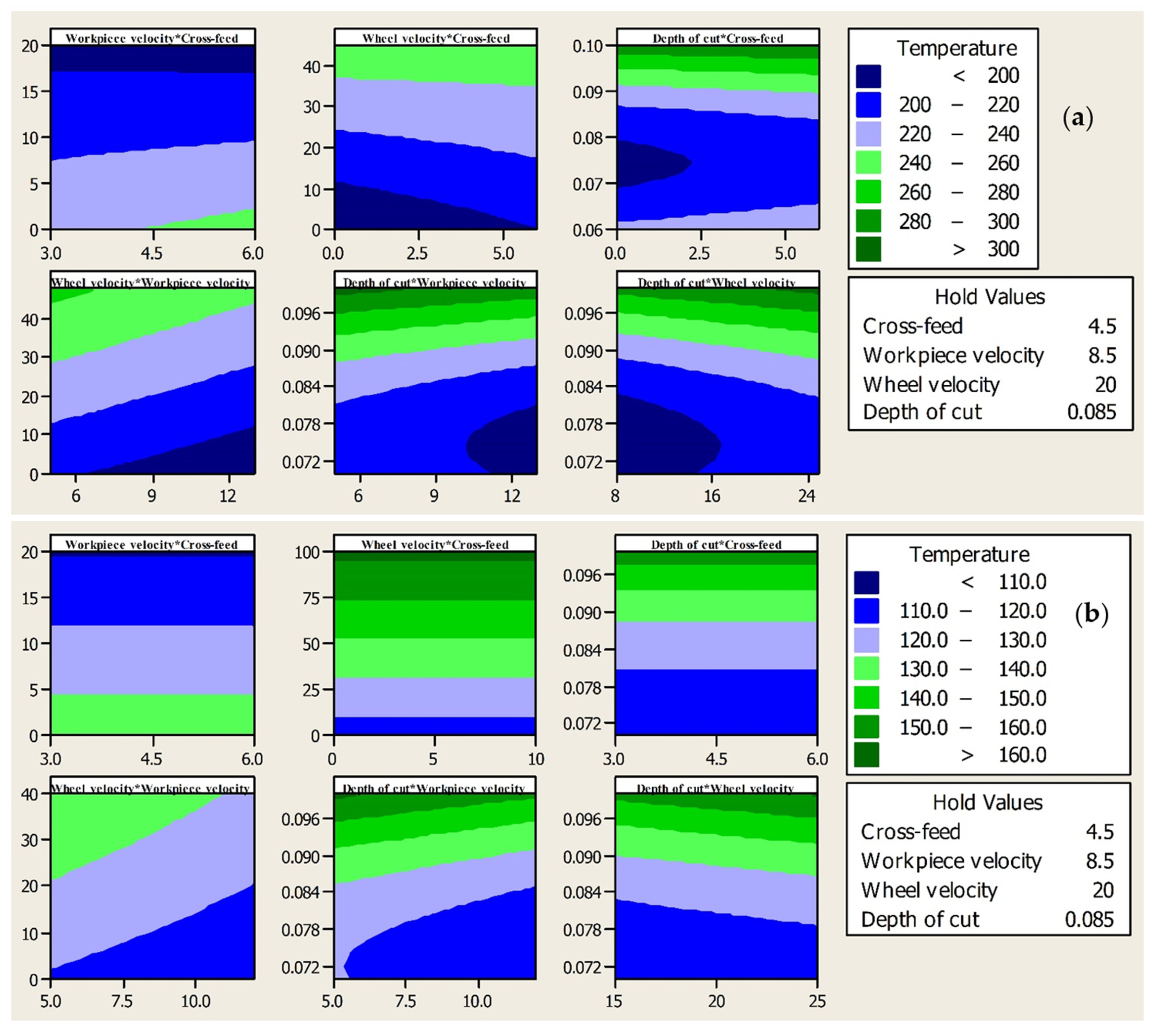
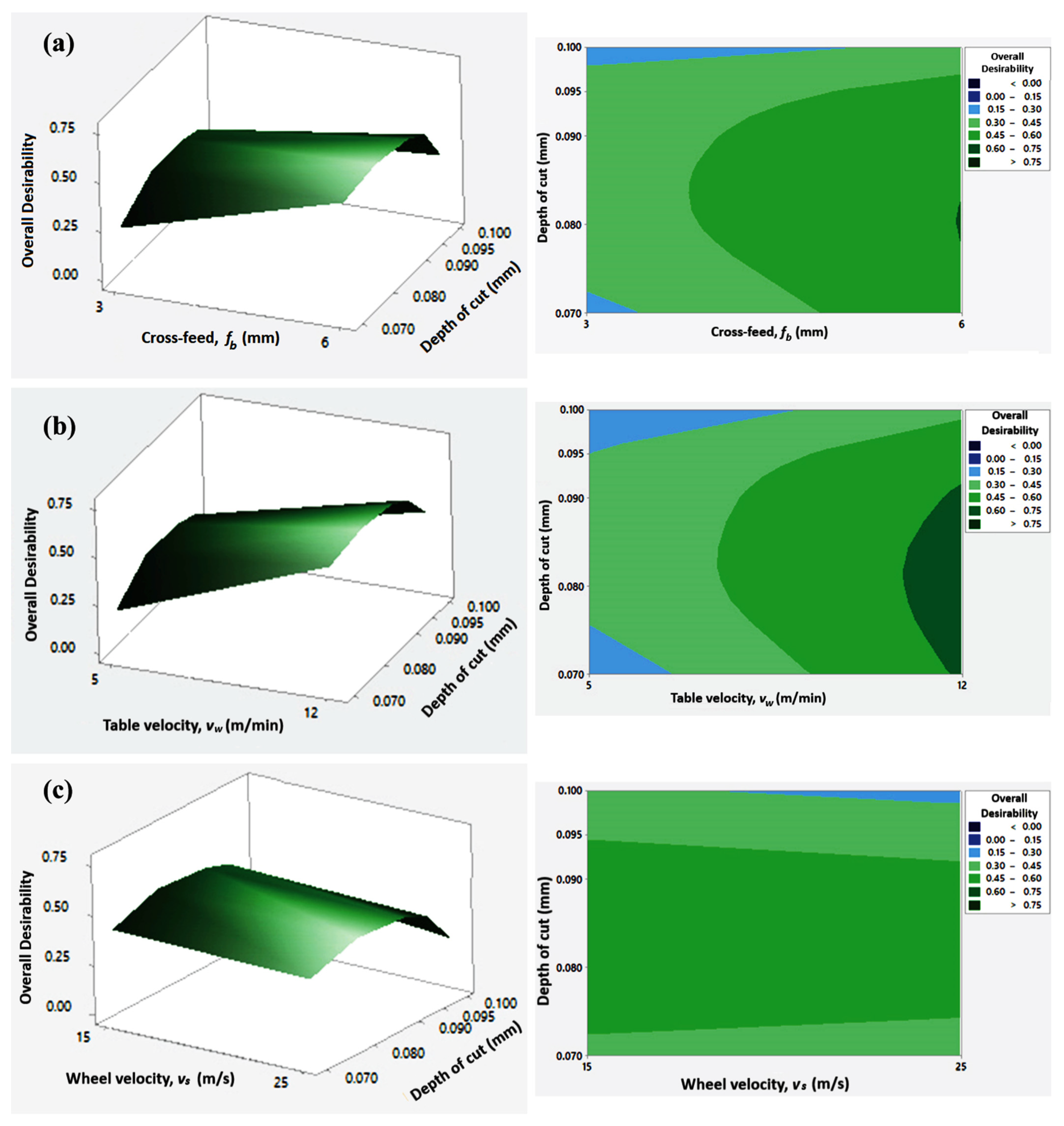
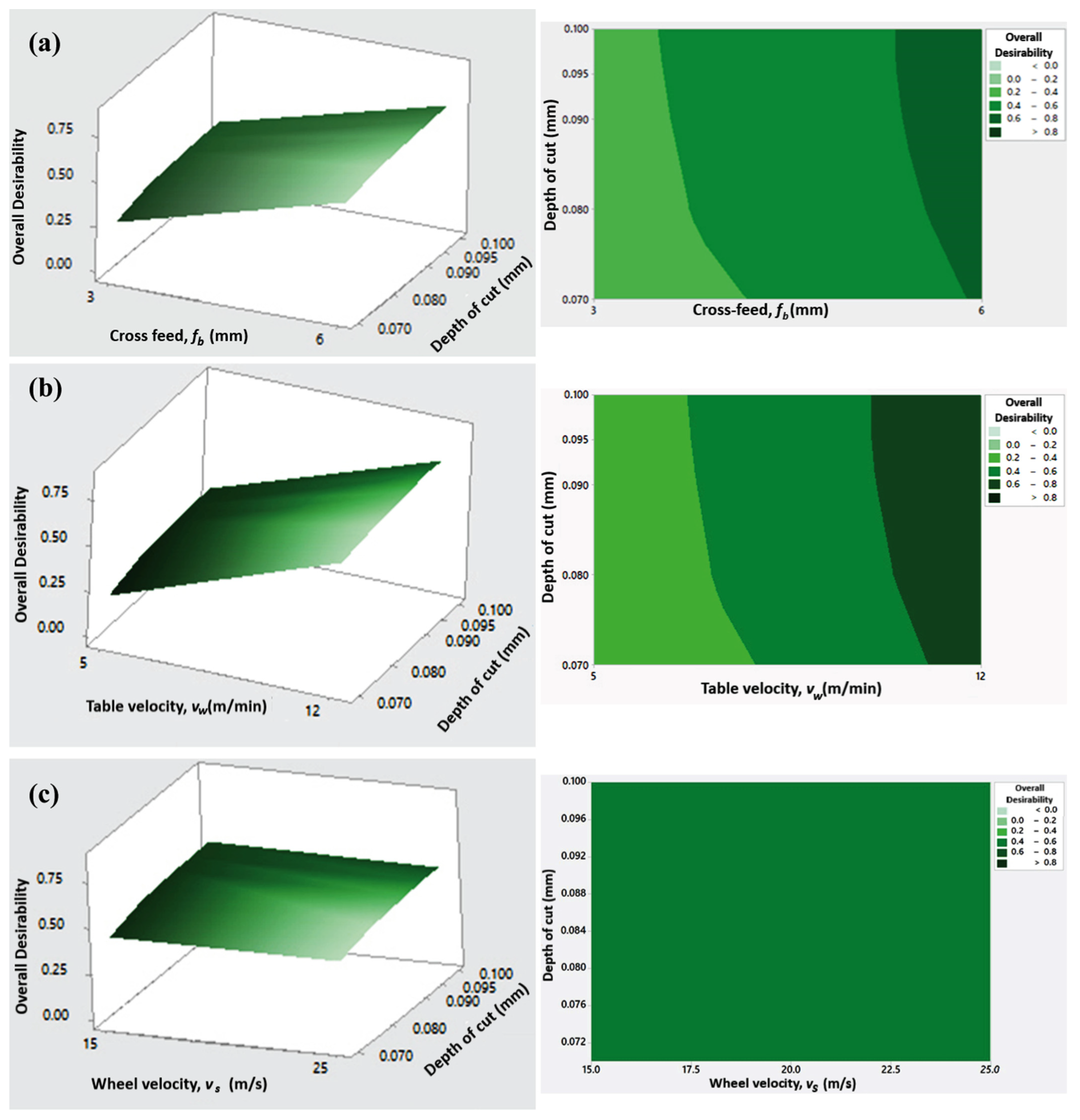
  • The wet condition dominates the overall desirability when the temperature is given the highest (≥20%) weightage. As our optimization goal was minimum temperature, the obtained result is as expected. Since the wet conditions keep the temperature down, the obtained result is achieved so. Again, in current scenario, cross-feed, wheel velocity, and depth of cut were at the lowest levels as a higher value of these parameter increases the amount of material removal per pass leading to increased temperature.
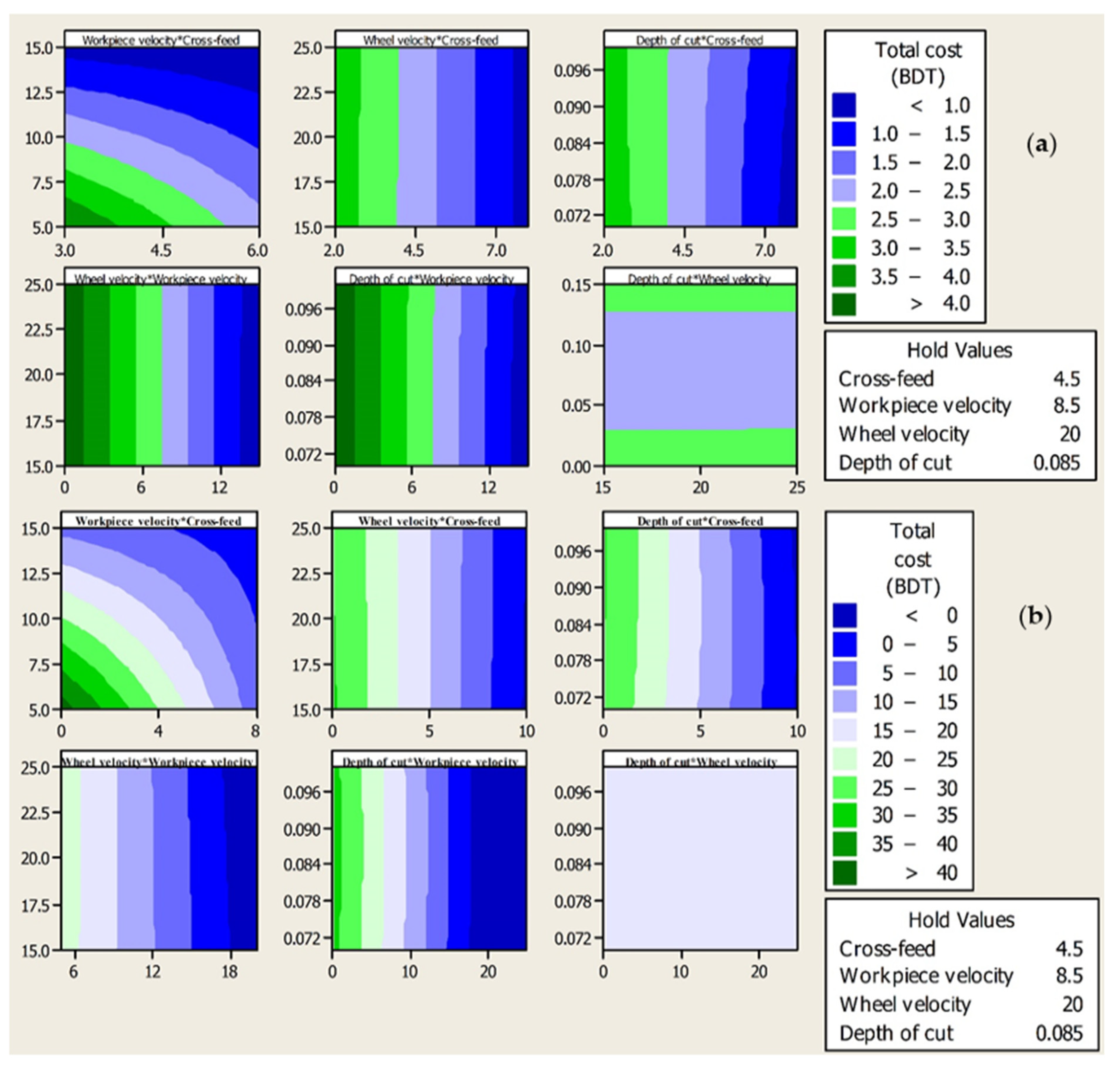
  • Dry condition achieves the highest overall desirability if the cost is given the highest priority instead. As the optimization goal was minimum cost, the obtained result is as expected. The underlying reason of the obtained result is no use of cutting fluid in the dry condition, hence cost is reduced. However, in the wet condition, cost is added due to cost of cutting fluid and extra power consumption. Again, in the current scenario, except depth of cut and wheel velocity, all other input parameters are at their upper limit. This provides a higher material removal leading to short machining time and reduced cost. However, depth of cut and wheel velocity at its upper limit provides larger power consumption which in turn increases cost. Thus, depth of cut and wheel velocity was kept at the lowest level.
  • If MRR is given priority (20:40:40), i.e., quick material removal, then all the input parameters are set at their highest level along with the wet machining condition. Larger MRR require higher cross-feed, depth of cut, wheel velocity, and higher workpiece velocity. Due to higher MRR, quick removal of chips is required which is very effective with wet machining condition. The obtained result exists at two levels of wheel velocity (15 and 25 m/s). At higher wheel velocity, grinding zone temperature is higher, which is expected. However, it may lead to poor surface quality. Hence, lower wheel velocity is found to be more suitable for grinding.
  • For equal weights of responses, the optimal values are found to be 6 mm/pass of cross-feed, 12 m/min of workpiece velocity, 15 m/s of the wheel or cutting velocity, 0.095 mm of the depth of cut in wet condition, with a maximum overall desirability value of 0.863. Optimum value for other weights of responses can be found in Table 8.
  • For dry cutting condition, keeping other parameters constant, desirability value increases with higher values of depth of cut until 0.095 mm, from where it decreases. This is because, up to a certain increase in depth of cut, high temperature is produced which drives the overall desirability down. If depth of cut is kept constant instead, then a positive relationship between the overall desirability values, and cross-feed and workpiece velocity is observed.
  • For the wet conditions, it is observed that workpiece velocity and cross-feed are positively related to the higher overall desirability values whereas the depth of cut and wheel velocity have negligible effects.
  • For a specific weight assignment, it is evident that the depth of cut positively affects the overall desirability values in the dry cutting condition, but it has a negligible effect in the wet condition.
  • It must be kept in mind that these conjectures are not invariable; rather it depends on how the weights are assigned. Wheel velocity has no apparent effect on desirability when all weights are equal in our case. However, this scenario will most likely change if different weights are assigned.
  • The confirmatory experiments corroborate that the predicted responses are in good agreement with the experimental results.
The presented study is helpful in setting the input parameters when any of the output responses is given more priority compared to rest. Most important output responses are given higher weightage than others to determine the corresponding input parameters while calculating the overall desirability. This model is highly flexible for the researchers and industrial practitioners to set input parameters if a particular response is given more focus. Again, as the results indicate, for higher MRR all the input parameter, i.e., cross-feed, wheel velocity, workpiece velocity, and depth of cut were set at the highest level for quick material removal where surface condition is not an issue of concern. This particular scenario is used in rough machining (manufacturing low category engineering products) for shortest machining time at the light engineering workshops in developing countries i.e., Bangladesh. Again, if surface condition (low grinding zone temperature) is given priority (manufacturing better quality product) weightage scheme 100:0:0 can be used. This model can be adopted by the light engineering workshops in developing countries, i.e., Bangladesh. Another interesting future research endeavor might include efforts to see how multi-response optimization of machining parameters turns out if different prediction models are used instead of RSM. Especially, a machine learning model might be a better predictor than RSM, given sufficient data for training.

5. Strength and Limitations of the Study

MRR and cost was calculated based on direct measurement, so these output responses were accurate at its best. However, the temperature was measured based on the developed thermocouple setup presented in the study. This set up has some strengths i.e., simple, rugged, easy to build the setup and relatively inexpensive. Further it can measure wide range of temperature and thermocouple junction can easily be inserted into the body cavity of the workpiece. So, the obtained temperature was best achieved as it was in direct contact with workpiece.
Besides, the developed setup has some limitations, i.e., limited accuracy and sensitivity, and is not convenient for practical applications. As mentioned at the experimental setup, the inserted pole into the workpiece cavity was insulated to avoid convection and radiation heat transfer, but it could not be fully nullified. Again, low voltage signals are susceptible to noise. As no shielding was there to stop noise, the results may have some errors.

Supplementary Materials

The following supporting information can be downloaded at: https://www.mdpi.com/article/10.3390/coatings12010104/s1, Table S1: Specifications of the workpiece and wheel used in the experiment; Table S2: Input parameters, their level and output units of each parameter; Table S3: Formula for calculating wheel velocity and MRR; Table S4: Raw data for the regression analysis under dry condition; Table S5: Raw data for the regression analysis under wet condition; Table S6: Data table showing design of experiment; Table S7: Data table showing the calculation of temperature using RSM equations; Table S8: Data table showing cost calculation under dry and wet condition using RSM equations; Table S9: Data table showing the calculation of desirability at dry condition; Table S10: Data table showing the calculation of desirability at wet condition.

Author Contributions

Conceptualization, R.R., S.K.G., T.I.K. and M.M.R.; methodology, R.R., S.K.G., T.I.K., S.H., M.M.R. and M.K.; software, S.K.G. and T.I.K.; validation, R.R., M.M.R. and T.I.K.; formal analysis, R.R., S.K.G., T.I.K. and M.M.R.; investigation, R.R. and T.I.K.; resources, R.R., M.K. and M.M.R.; data curation, R.R.; writing—original draft preparation, R.R.; writing—review and editing, M.M.R., S.K.G., T.I.K., T.A. and M.K.; visualization, S.H.; supervision, M.M.R.; project administration, M.M.R., M.A. and M.K.; funding acquisition, M.A. and M.K. All authors have read and agreed to the published version of the manuscript.

Funding

This work was supported by the National Research Foundation of Korea (NRF), grant funded by the Korea government (MSIT) (No. NRF-2019R1G1A1099335).

Institutional Review Board Statement

Not applicable.

Informed Consent Statement

Not applicable.

Data Availability Statement

Data sharing is not applicable to this article.

Acknowledgments

The authors are grateful to the Department of Industrial and Production Engineering, BUTEX for permitting to employ the lab facilities to conduct all the necessary experiments.

Conflicts of Interest

The authors declare no conflict of interest.

Nomenclature

apdepth of cut (mm)
bwidth of the cut (mm)
b0, bi, bii, bijcoefficient of intercept, linear, quadratic and interaction of input variables respectively
bjo, bjk, bjkk, bjklare the regression coefficients
Costdrytotal cost at dry machining condition (BDT)
Costwettotal cost at wet machining condition (BDT)
Dioverall desirability of all responses
apithe depth of cut at experiment i
d i j ( Y ^ i j ) = 0denotes the lowest desirability value of output response (Yij)
d i j ( Y ^ i j ) = 1denotes the highest desirability value of output response (Yij)
fbcross-feed (mm/pass)
fbicross-feed at experiment i
Gijtarget value of the jth response (Yij)
0 d i j ( Y ^ i j ) 1
G i j m a x maximum goal of output j at experiment i
G i j m i n minimum goal of output j at experiment i
mno. of experimental runs
Mijlower level of output j at experiment i
MRRmaterial removal rate (mm3/s)
nno. of output responses variables
Nijhigher level of output j at experiment i
pno. of input independent parameters
TempdryTemperature at dry machining condition (°C)
TempwetTemperature at wet machining condition (°C)
vswheel velocity (m/s)
vsithe wheel velocity at experiment i
vwworkpiece velocity or longitudinal table travel velocity (m/min)
vwiworkpiece velocity at experiment i
Yijoutput responses value at ith experiment of jth response, j = 1, 2,…, n

References

  1. Chattopadhyay, A. Machining and Machine Tools (With CD); John Wiley & Sons: Hoboken, NJ, USA, 2011. [Google Scholar]
  2. Gupta, M.K.; Khan, A.M.; Song, Q.; Liu, Z.; Khalid, Q.S.; Jamil, M.; Kuntoğlu, M.; Usca, Ü.A.; Sarıkaya, M.; Pimenov, D.Y. A review on conventional and advanced minimum quantity lubrication approaches on performance measures of grinding process. Int. J. Adv. Manuf. Technol. 2021, 117, 729–750. [Google Scholar] [CrossRef]
  3. Malkin, S.; Guo, C. Grinding Technology: Theory and Application of Machining with Abrasives; Industrial Press Inc.: New York, NY, USA, 2008. [Google Scholar]
  4. Leskovar, P.; Grum, J. The metallurgical aspects of machining. CIRP Ann. 1986, 35, 537–550. [Google Scholar] [CrossRef]
  5. Tönshoff, H.; Brinksmeier, E. Determination of the mechanical and thermal influences on machined surfaces by microhardness and residual stress analysis. CIRP Ann. 1980, 29, 519–530. [Google Scholar] [CrossRef]
  6. Rowe, W.B. Principles of Modern Grinding Technology; William Andrew: Norwich, NY, USA, 2013. [Google Scholar]
  7. Guo, G.; Liu, Z.; An, Q.; Chen, M. Experimental investigation on conventional grinding of Ti-6Al-4V using SiC abrasive. Int. J. Adv. Manuf. Technol. 2011, 57, 135–142. [Google Scholar] [CrossRef]
  8. Howes, T.; Tönshoff, H.; Heuer, W.; Howes, T. Environmental aspects of grinding fluids. CIRP Ann. 1991, 40, 623–630. [Google Scholar] [CrossRef]
  9. Jawahir, I.; Brinksmeier, E.; M’saoubi, R.; Aspinwall, D.; Outeiro, J.; Meyer, D.; Umbrello, D.; Jayal, A. Surface integrity in material removal processes: Recent advances. CIRP Ann. 2011, 60, 603–626. [Google Scholar] [CrossRef]
  10. Sharma, C.; Ghosh, S.; Talukdar, P. Finite element analysis of workpiece temperature during surface grinding of inconel 718 alloy. In Proceedings of the 5th International & 26th All India Manufacturing Technology, Design and Research Conference, IIT Guwahati, Assam, India, 12–14 December 2014; pp. 420–421. [Google Scholar]
  11. Guo, C.; Wu, Y.; Varghese, V.; Malkin, S. Temperatures and energy partition for grinding with vitrified CBN wheels. CIRP Ann. 1999, 48, 247–250. [Google Scholar] [CrossRef]
  12. Upadhyaya, R.; Malkin, S. Thermal aspects of grinding with electroplated CBN wheels. J. Manuf. Sci. Eng. 2004, 126, 107–114. [Google Scholar] [CrossRef]
  13. Yao, C.; Wang, T.; Xiao, W.; Huang, X.; Ren, J. Experimental study on grinding force and grinding temperature of Aermet 100 steel in surface grinding. J. Mater. Process. Technol. 2014, 214, 2191–2199. [Google Scholar] [CrossRef]
  14. Johnson, R.T.; Parker, P.A.; Montgomery, D.C.; Cutler, A.D.; Danehy, P.M.; Rhew, R.D. Design strategies for response surface models for the study of supersonic combustion. Qual. Reliab. Eng. Int. 2009, 25, 365–377. [Google Scholar] [CrossRef]
  15. Bhushan, R.K. Optimization of cutting parameters for minimizing power consumption and maximizing tool life during machining of Al alloy SiC particle composites. J. Clean. Prod. 2013, 39, 242–254. [Google Scholar] [CrossRef]
  16. Rudrapati, R.; Pal, P.K.; Bandyopadhyay, A. Modeling and optimization of machining parameters in cylindrical grinding process. Int. J. Adv. Manuf. Technol. 2016, 82, 2167–2182. [Google Scholar] [CrossRef]
  17. Janardhan, M.; Krishna, A.G. Multi-objective optimization of cutting parameters for surface roughness and metal removal rate in surface grinding using response surface methodology. Int. J. Adv. Eng. Technol. 2012, 3, 270. [Google Scholar]
  18. Periyasamy, S.; Aravind, M.; Vivek, D.; Amirthagadeswaran, K. Optimization of Surface Grinding Process Parameters for Minimum Surface Roughness in AISI 1080 Using Response Surface Methodology. Adv. Mater. Res. 2014, 984–985, 118–123. [Google Scholar] [CrossRef]
  19. Venkatesan, K.; Devendiran, S.; Sachin, D.; Swaraj, J. Investigation of machinability characteristics and comparative analysis under different machining conditions for sustainable manufacturing. Measurement 2020, 154, 107425. [Google Scholar] [CrossRef]
  20. Manohar, M.; Joseph, J.; Selvaraj, T.; Sivakumar, D. Application of desirability-function and RSM to optimise the multi-objectives while turning Inconel 718 using coated carbide tools. Int. J. Manuf. Technol. Manag. 2013, 27, 218–237. [Google Scholar] [CrossRef]
  21. Naresh, N.; Rajasekhar, K. Multi-response optimization for milling AISI 304 Stainless steel using GRA and DFA. Adv. Mater. Res. 2016, 5, 67–80. [Google Scholar] [CrossRef]
  22. Buranská, E.; Buranský, I. Cutting Environment Impact on the Aluminium Alloy Machining (DFA). In Proceedings of the 29th DAAAM International Symposium, Zadar, Croatia, 21–28 October 2018; pp. 1158–1163. [Google Scholar]
  23. Borchers, F.; Clausen, B.; Eckert, S.; Ehle, L.; Epp, J.; Harst, S.; Hettig, M.; Klink, A.; Kohls, E.; Meyer, H.; et al. Comparison of Different Manufacturing Processes of AISI 4140 Steel with Regard to Surface Modification and Its Influencing Depth. Metals 2020, 10, 895. [Google Scholar] [CrossRef]
  24. Saravanan, R.; Asokan, P.; Sachidanandam, M. A multi-objective genetic algorithm (GA) approach for optimization of surface grinding operations. Int. J. Mach. Tools Manuf. 2002, 42, 1327–1334. [Google Scholar] [CrossRef]
  25. Pawar, P.; Rao, R.; Davim, J. Multiobjective optimization of grinding process parameters using particle swarm optimization algorithm. Mater. Manuf. Process. 2010, 25, 424–431. [Google Scholar] [CrossRef]
  26. Alajmi, M.S.; Alfares, F.S.; Alfares, M.S. Selection of optimal conditions in the surface grinding process using the quantum based optimisation method. J. Intell. Manuf. 2019, 30, 1469–1481. [Google Scholar] [CrossRef]
  27. Zhang, G.; Liu, M.; Li, J.; Ming, W.; Shao, X.; Huang, Y. Multi-objective optimization for surface grinding process using a hybrid particle swarm optimization algorithm. Int. J. Adv. Manuf. Technol. 2014, 71, 1861–1872. [Google Scholar] [CrossRef]
  28. Gholami, M.H.; Azizi, M.R. Constrained grinding optimization for time, cost, and surface roughness using NSGA-II. Int. J. Adv. Manuf. Technol. 2014, 73, 981–988. [Google Scholar] [CrossRef]
  29. Khalilpourazari, S.; Khalilpourazary, S. Optimization of time, cost and surface roughness in grinding process using a robust multi-objective dragonfly algorithm. Neural Comput. Appl. 2020, 32, 3987–3998. [Google Scholar] [CrossRef]
  30. Öztürk, S.; Kahraman, M.F. Modeling and optimization of machining parameters during grinding of flat glass using response surface methodology and probabilistic uncertainty analysis based on Monte Carlo simulation. Measurement 2019, 145, 274–291. [Google Scholar] [CrossRef]
  31. Shin, T.M.; Adam, A.; Abidin, A.F.Z. A comparative study of PSO, GSA and SCA in parameters optimization of surface grinding process. Bull. Electr. Eng. Inform. 2019, 8, 1117–1127. [Google Scholar] [CrossRef]
  32. Bardhan, P.K.; Bhunia, B.; Goswami, S.; Chandra, P. Optimization of Process Parameters of Surface Grinding of AISI 304 Steel with Al2O3 Abrasive Wheel. In Proceedings of the International Conference on Industry Interactive Innovations in Science, Engineering and Technology (I3SET2K19), Kalyani, India, 13–14 December 2019. [Google Scholar]
  33. Sanjeevi, R.; Kumar, G.A.; Krishnan, B.R. Optimization of machining parameters in plane surface grinding process by response surface methodology. Mater. Today Proc. 2020, 37, 85–87. [Google Scholar] [CrossRef]
  34. Dambatta, Y.S.; Sayuti, M.; Sarhan, A.A.; Hamdi, M. Comparative study on the performance of the MQL nanolubricant and conventional flood lubrication techniques during grinding of Si3N4 ceramic. Int. J. Adv. Manuf. Technol. 2018, 96, 3959–3976. [Google Scholar] [CrossRef]
  35. Maier, M.; Rupenyan, A.; Bobst, C.; Wegener, K. Self-optimizing grinding machines using Gaussian process models and constrained Bayesian optimization. Int. J. Adv. Manuf. Technol. 2020, 108, 539–552. [Google Scholar] [CrossRef]
  36. Ronoh, K.N.; Mwema, F.M.; Akinlabi, S.A.; Akinlabi, E.T.; Karuri, N.W.; Ngetha, H.T. Effects of cooling conditions and grinding depth on sustainable surface grinding of Ti-6Al-4V: Taguchi approach. AIMS Mater. Sci. 2019, 6, 697–712. [Google Scholar] [CrossRef]
  37. Tung, L.A.; Pi, V.N.; Ha, D.T.T.; Hung, L.X.; Banh, T.L. A study on optimization of surface roughness in surface grinding 9CrSi tool steel by using Taguchi method. In Advances in Engineering Research and Application, Proceedings of the International Conference on Engineering Research and Applications, ICERA 2019, Thai Nguyen, Vietnam, 1–2 December 2019; Sattler, K.-U., Nguyen, D.C., Vu, N.P., Long, B.T., Puta, H., Eds.; Springer: Cham, Switzerland, 2020; pp. 100–108. [Google Scholar]
  38. Singh, H.; Sharma, V.S.; Dogra, M. Exploration of graphene assisted vegetables oil based minimum quantity lubrication for surface grinding of TI-6AL-4V-ELI. Tribol. Int. 2020, 144, 106113. [Google Scholar] [CrossRef]
  39. Patil, P.J.; Patil, C. Analysis of process parameters in surface grinding using single objective Taguchi and multi-objective grey relational grade. Perspect. Sci. 2016, 8, 367–369. [Google Scholar] [CrossRef] [Green Version]
  40. Rabiei, F.; Rahimi, A.; Hadad, M.; Ashrafijou, M. Performance improvement of minimum quantity lubrication (MQL) technique in surface grinding by modeling and optimization. J. Clean. Prod. 2015, 86, 447–460. [Google Scholar] [CrossRef]
  41. Rabiei, F.; Rahimi, A.; Hadad, M. Performance improvement of eco-friendly MQL technique by using hybrid nanofluid and ultrasonic-assisted grinding. Int. J. Adv. Manuf. Technol. 2017, 93, 1001–1015. [Google Scholar] [CrossRef]
  42. Puri, A.B.; Banerjee, S. Multiple-response optimisation of electrochemical grinding characteristics through response surface methodology. Int. J. Adv. Manuf. Technol. 2013, 64, 715–725. [Google Scholar] [CrossRef]
  43. Khan, A.M.; Jamil, M.; Mia, M.; Pimenov, D.Y.; Gasiyarov, V.R.; Gupta, M.K.; He, N. Multi-objective optimization for grinding of AISI D2 steel with Al2O3 wheel under MQL. Materials 2018, 11, 2269. [Google Scholar] [CrossRef] [PubMed] [Green Version]
  44. Palanikumar, K. Modeling and analysis for surface roughness in machining glass fibre reinforced plastics using response surface methodology. Mater. Des. 2007, 28, 2611–2618. [Google Scholar] [CrossRef]
  45. Celep, O.; Aslan, N.; Alp, İ.; Taşdemir, G. Optimization of some parameters of stirred mill for ultra-fine grinding of refractory Au/Ag ores. Powder Technol. 2011, 208, 121–127. [Google Scholar] [CrossRef]
  46. Krajnik, P.; Kopac, J.; Sluga, A. Design of grinding factors based on response surface methodology. J. Mater. Process. Technol. 2005, 162, 629–636. [Google Scholar] [CrossRef]
  47. Pradhan, M.K.; Biswas, C.K. Modeling of residual stresses of EDMed AISI 4140 Steel. In Proceedings of the International Conference on Recent Advances in Materials, Processing and Characterization, VRS Engineering College, Vijayawada, India, 3–4 July 2008; pp. 49–55. [Google Scholar]
  48. Khuri, A.I. 12 Multiresponse surface methodology. Handb. Stat. 1996, 13, 377–406. [Google Scholar]
  49. Harrington, E.C. The desirability function. Ind. Qual. Control 1965, 21, 494–498. [Google Scholar]
  50. Derringer, G.; Suich, R. Simultaneous optimization of several response variables. J. Qual. Technol. 1980, 12, 214–219. [Google Scholar] [CrossRef]
  51. Pignatiello Jr, J.J. Strategies for robust multiresponse quality engineering. IIE Trans. 1993, 25, 5–15. [Google Scholar] [CrossRef]
  52. Ryan, T.P.; Morgan, J. Modern experimental design. J. Stat. Theory Pract. 2007, 1, 501–506. [Google Scholar] [CrossRef]
  53. Sadeghi, M.; Hadad, M.; Tawakoli, T.; Vesali, A.; Emami, M. An investigation on surface grinding of AISI 4140 hardened steel using minimum quantity lubrication-MQL technique. Int. J. Mater. Form. 2010, 3, 241–251. [Google Scholar] [CrossRef]
Figure 1. Flow chart of current research.
Coatings 12 00104 g001
Figure 2. A schematic diagram depicting the design of experiment (DOE) conducted for this research work. (a) shows high low level of the parameters and (b) shows the multilevel full factorial design (24 × 5 = 80) applied to run 80 experiments.
Coatings 12 00104 g002
Figure 3. (a) Schematic diagram of the experimental setup where inset A and B shows photograph images workpiece before slot cutting and after slot cutting using wire EDM, and (b) pictorial view of the experimental setup. A—Workpiece before machining. B—Wire cut on the workpiece. 1—Thermocouple setup on the workpiece. 2—Dry machining setup. 3—Wet machining setup. 4—Workpiece after machining.
Coatings 12 00104 g003
Figure 4. A flowchart showing RSM methodology.
Coatings 12 00104 g004
Figure 5. Flowchart of DFA methodology.
Coatings 12 00104 g005
Figure 6. Contour plot of the temperature for each combination of input parameters. (a) Surface grinding under dry condition and (b) surface grinding under wet condition.
Coatings 12 00104 g006
Figure 7. Contour plot of the total cost for each combination of input parameters. (a) Surface grinding under dry condition and (b) surface grinding under wet condition.
Coatings 12 00104 g007
Figure 8. Surface plot of individual desirability (a) for temperature in wet condition, and (b) for MRR in wet condition.
Coatings 12 00104 g008
Figure 9. Surface plot and corresponding contour plot for overall desirability in dry condition. (a) show the combined effect of cross-feed and depth of cut, (b) table velocity and depth of cut and (c) wheel velocity and depth of cut on overall desirability.
Coatings 12 00104 g009
Figure 10. Surface plot and corresponding contour plot for overall desirability in wet condition (equal weightage). (a) show the combined effect of cross-feed and depth of cut, (b) table velocity and depth of cut and (c) wheel velocity and depth of cut on overall desirability.
Coatings 12 00104 g010
Table 1. Grinding process parameters optimization using different analysis techniques in the literature.
Type of GrindingMaterial UsedParameter OptimizedOptimized OutputAnalysis TechniqueRef.
Dry grindingMild steelWheel speed, workpiece speed, depth of dressing and lead of dressingMinimum production cost, maximum production rate and the finest possible surface grinding finishGenetic Algorithm (GA)[24]
Mild SteelWheel speed, workpiece speed, depth of dressing and lead of dressingProduction cost, production rate and surface finishParticle swarm optimization (PSO) algorithm[25]
Mild SteelWheel speed, workpiece speed, depth of dressing and lead of dressingProduction cost, production rate and surface finishQuantum Based Optimization Method (QBOM)[26]
Mild SteelWheel speed, workpiece speed, depth of dressing and lead of dressingProduction cost, production rate and surface roughnessHybrid Particle Swarm Optimization (HPSO) algorithm[27]
1.2080 SteelWheel speed, workpiece speed and depth of cutSurface finish, total grinding time and production costNon-dominated sorting genetic algorithm (NSGA II)[28]
1.2080 SteelWheel speed, workpiece speed and depth of cutSurface quality, total grinding time and production costDragonfly algorithm[29]
EN24 steelWheel speed, table speed and depth of cutSurface roughness and metal removal rateRSM optimization[17]
Soda-lime glassWheel speed, depth of cut and feed rateSurface roughnessRSM and Monte Carlo Simulation[30]
SteelSpeed of wheel, speed of workpiece, depth of dressing and lead of dressingProduction cost, production rate and surface finishParticle swarm optimization, Gravitational search algorithm and Sine Cosine algorithm[31]
Stainless steel material AISI 304Feed rate, speed of table and depth of cutMRR and surface roughnessANOVA, Taguchi method[32]
EN 24 steelWheel speed, depth of cut and feed rate timingSurface roughnessRSM[33]
Conventional grindingSilicon nitride ceramicFeed rate, depth of cut, type of diamond wheel and lubrication typeGrinding forces, workpiece surfaceroughness, surface damages and wheel wearAdaptiveneuro-fuzzy inference system (ANFIS) and Taguchi method[34]
Tungsten carbide insertFeed rate and cutting speedProduction costs, grinding burn, surface roughness and temperature at the grinding surfaceConstrained Bayesian optimization combined with Gaussian process Models[35]
Ti-6Al-4VCoolant types, cooling techniques and grinding depthsSurface hardness and surface morphologyTaguchi method and ANOVA[36]
9CrSi annealing tool steelCoolant concentration, coolant flow, cross-feed, table speed and depth of cutSurface roughnessTaguchi method[37]
Ti-6Al-4V-ELITypes of coolant and graphene percentage in the coolantSurface roughness, grinding force, specific grinding energy and coefficient-of-frictionExperimental (conventional)[38]
MQL grindingEN8 flat plateDepth of cut, type of lubricant, feed rate, grinding wheel speed, coolant flow rate and nanoparticlesizeG ratio and surface finishTaguchi based Grey relational analysis, ANOVA[39]
Two soft steels (CK45 and S305) and two hard steels (HSS and 100Cr6)Depth of cut, cutting speed and feed rateGrinding forces, friction coefficient, surface roughness, surface morphology and form of the chipsRSM, ANOVA, GA[40]
Electrochemical grinding100Cr6 hardened steel (bearing steel)Specific material removal rateMaximum temperature, grinding forces and friction coefficientExperimental (conventional)[41]
Composite carbide insertsVoltage and cutting speedCurrent density, material removal rate (MRR) and surface finishResponse surface methodology (RSM), Desirability function[42]
Table 2. Chemical composition and properties of the workpiece material.
PropertiesSpecification
Work materialAISI 4140 alloy steel
Dimension72 mm × 37 mm × 27.3 mm
TypeSolid
Chemical compositionCarbonChromiumIronManganeseMolybdenumPhosphorousSiliconSulfur
0.380–0.4300.8–1.10Balance0.75–1.00.15–0.250.0350.15–0.300.040
Hardness40 HRC
Tensile strength655 MPa
Yield strength415 MPa
Hardness, Brinell197
Density7.85 g/cm3
Melting point1416 °C
Table 3. Grinding conditions.
Grinding Conditions with SpecificationGrinding modeSingle pass surface grinding, down cut
Grinding machineOkamoto hydraulic surface grinder
Nozzle angle15°
Flow rate5 L/min
Flow measuring deviceZ-5615 Panel Flowmeter
Machining conditionDry, Wet (Flood)
Labor cost0.06 BDT/s
Power consumption cost8 BDT/unit
Cutting fluid cost0.5 BDT/s
Dressing Cut ParameterDresserSingle point diamond, HS050
Total depth of dressing300 μm
Dressing speed400 mm/min
Grinding wheel wear per dress, radially3.75 μm
Table 4. Input parameters and their levels.
SI. No.Grinding Input ParametersLevel 1Level 2Level 3Level 4Level 5
1Workpiece velocity, vw (m/min)512---
2Wheel velocity, vs (m/s)1525---
3Depth of cut, ap (mm)0.070.080.090.0950.10
4Cross-feed, fb (mm/pass)36---
5Cutting conditionDryWet---
Table 5. Optimum range of input parameters from RSM.
ObjectivesParameters/
Condition
Workpiece Velocity, vw (m/min)Wheel Velocity,
vs (m/s)
Depth of Cut, ap mmCross-Feed, fb (mm/Pass)
The optimum level for tempDry12–202–100.065–0.0850.1–2.5
The optimum level for the cost12–15-0.03–0.136.5–8
The optimum level for tempWet15–201–120.062–0.080-
The optimum level for the cost15–20--7–10
Table 6. Optimization criteria for input parameters.
Variable TypeVariablesTargetLower BoundUpper Bound
Independent (input parameters)Cutting conditionDry or WetN/AN/A
Cross-feed (mm/pass)In range36
Workpiece velocity (m/min)In range512
Wheel velocity (m/s)In range1525
Depth of cut (mm)In range0.070.10
Dependent (response)Temperature (°C)Minimize109.78313.67
MRR (mm3/min)Maximize10507200
Total cost (BDT)Minimize0.9129.48
Table 7. Individual and overall desirability values for three different cases.
Individual DesirabilityOverall Desirability (Equal Weightage 33:33:33)Overall Desirability
(20:40:40)
Overall Desirability (15:25:60)
Temp.MRRTotal Cost
0.53300.890000
0.5270.0250.8910.2280.1930.338
0.3770.0490.8910.2550.2360.380
0.2490.0610.8910.2390.2370.377
0.0860.0740.8910.1790.2070.337
0.45800.888000
0.4560.0250.8900.2170.1870.330
0.3120.0490.8900.2400.2270.369
0.1860.0610.8900.2170.2230.361
0.0240.0740.8900.1170.1600.278
0.6150.2400.9690.5240.5070.639
0.6010.2980.9700.5590.5500.673
0.4440.3570.9700.5370.5570.672
0.3110.3860.9700.4890.5350.650
0.1440.4150.9700.3880.4720.590
0.5420.2400.9680.5020.4940.627
0.5320.2980.9690.5360.5370.660
0.3790.3570.9690.5090.5390.656
0.2490.3860.9690.4540.5110.628
0.0840.4150.9690.3240.4240.544
0.4870.1710.9540.4310.4200.562
0.4840.2200.9530.4670.4630.597
0.3390.2690.9530.4440.4680.595
0.2130.2930.9510.3910.4410.567
0.0520.3180.9510.2510.3440.468
0.4230.1710.9530.4110.4080.550
0.4250.2200.9520.4470.4510.585
0.2840.2690.9510.4180.4510.579
0.1600.2930.9500.3550.4160.542
0.0010.3180.9500.0680.1560.259
0.5910.6490.9950.7260.7560.827
0.5800.7660.9940.7620.8050.860
0.4270.8830.9920.7210.8000.850
0.2970.9420.9920.6530.7640.818
0.1321.0000.9910.5080.6650.735
0.5280.6490.9930.6990.7390.813
0.5220.7660.9920.7350.7870.845
0.3730.8830.9910.6890.7790.832
0.2460.9420.9900.6130.7350.794
0.0821.0000.9890.4340.6040.683
0.95100.052000
0.9420.0250.0310.0910.0570.050
0.8820.0490.0220.0990.0640.047
0.8320.0610.0220.1040.0690.049
0.7700.0740.0240.1120.0760.054
0.94300.030000
0.9230.0250.0180.0750.0460.036
0.8500.0490.0160.0880.0560.039
0.7950.0610.0200.1000.0660.046
0.7270.0740.0260.1130.0770.056
0.9910.2400.6030.5240.4610.517
0.9850.2980.5830.5560.4960.534
0.9270.3570.5730.5750.5230.548
0.8790.3860.5720.5800.5330.553
0.8180.4150.5750.5810.5420.559
0.9880.2400.6100.5260.4630.520
0.9700.2980.5970.5580.4990.540
0.9000.3570.5950.5770.5270.558
0.8470.3860.5980.5810.5390.565
0.7800.4150.6050.5820.5480.572
0.9510.1710.5000.4340.3710.422
0.9420.2200.4850.4660.4040.440
0.8820.2690.4810.4860.4310.456
0.8320.2930.4840.4910.4420.464
0.7700.3180.4890.4940.4510.471
0.9430.1710.4670.4230.3600.404
0.9230.2200.4600.4550.3940.425
0.8500.2690.4650.4750.4220.444
0.7950.2930.4710.4800.4330.453
0.7270.3180.4800.4810.4430.461
0.9910.6490.7920.7990.7650.780
0.9850.7660.7760.8370.8100.802
0.9270.8830.7720.8590.8450.821
0.8790.9420.7740.8630.8590.829
0.8181.0000.7790.8610.8700.836
0.9880.6490.7870.7970.7630.776
0.9700.7660.7790.8340.8090.802
0.9000.8830.7830.8540.8450.824
0.8470.9420.7890.8580.8600.834
0.7801.0000.7980.8540.8700.842
Table 8. Optimum cutting parameters and corresponding responses for different weights.
Weights (%)Cutting ConditionCross-Feed (mm/pass)Workpiece Velocity (m/min)Wheel Velocity (m/s)Depth of Cut (mm)Temp. (°C)MRR (mm3/min)Total Cost (BDT)Overall Desirability
33.33:33.33:33.33 (Equal)Wet612150.095140.85468408.360.863
20:40:40Wet612150.100143.94572007.770.870
(tied)
612250.100150.11972006.32
15:25:60Dry612150.080204.56557601.010.860
100:0:0
(temperature only)
Wet312150.070109.785252012.240.991
0:0:100
(total cost only)
Dry612150.070191.79950401.080.995
Table 9. Comparison of predicted and experimental responses using DFA method.
SchemesCutting ConditionOptimum Cutting ParametersOptimum Process ParametersAbsolute Error (%)
Experimental ValuesPredicted Values
Weights (%)Temp. (°C)Total Cost (BDT)Overall DesirabilityTemp.
(°C)
Total Cost (BDT)Overall DesirabilityTemp. (°C)Total Cost (BDT)Overall Desirability
33.33:33.33:
33.33 (Equal)
Wet(fb, vw, vs, ap)
= (6, 12, 15, 0.095)
140.8548.360.863134.5557.3660.8444.477.372.2
20:40:40Wet(fb, vw, vs, ap)
= (6, 12, 15, 0.1)
143.9457.770.870
(tied)
146.9547.2260.8642.087.230.69
(fb, vw, vs, ap)
= (6, 12, 25, 0.1)
150.1196.32154.7716.690.8673.0995.850.35
15:25:60Dry(fb, vw, vs, ap)
= (6, 12, 15, 0.08)
204.5651.010.860195.431.090.8524.467.90.93
100:0:0 (temperature only)Wet(fb, vw, vs, ap)
= (3, 12, 15, 0.07)
109.78512.240.991111.6912.250.9891.730.160.20
0:0:100 (total cost only)Dry(fb, vw, vs, ap)
= (6, 12, 15, 0.07)
191.7991.080.995193.331.080.9940.8000.10
Publisher’s Note: MDPI stays neutral with regard to jurisdictional claims in published maps and institutional affiliations.

