Nanomechanical Concepts in Magnetically Guided Systems to Investigate the Magnetic Dipole Effect on Ferromagnetic Flow Past a Vertical Cone Surface

Abstract

Because of the floating magnetic nanomaterial, ferrofluids have magneto-viscous properties, enabling controllable temperature changes as well as nano-structured fluid characteristics. The study’s purpose is to evolve and solve a theoretical model of bioconvection nanofluid flow with a magnetic dipole effect in the presence of Curie temperature and using the Forchheimer-extended Darcy law subjected to a vertical cone surface. The model also includes the nonlinear thermal radiation, heat suction/injection, viscous dissipation, and chemical reaction effects. The developed model problem is transformed into nonlinear ordinary differentials, which have been solved using the homotopy analysis technique. In this problem, the behavior of function profiles are graphically depicted and explained for a variety of key parameters. For a given set of parameters, tables representthe expected numerical values and behaviors of physical quantities. The nanofluid velocity decreases as the ferrohydrodynamic, local inertia, and porosity parameters increase and decrease when the bioconvection Rayleigh number increases. Many key parameters improved the thermal boundary layer and temperature. The concentration is low when the chemical reaction parameter and Schmidt number rises. Furthermore, as the bioconvection constant, Peclet and Lewis numbers rise, so does the density of motile microorganisms.

1. Introduction

Fluids that are often magnetized by the existence of an exterior magnetic field are known as ferrofluids, which is an abbreviation for fluid and ferromagnetic particles. These fluids are made up of colloidal fluids formed of nanosized ferromagnetic or ferrimagnetic particles that have been stopped inside the fluid transporter. Brownian motion causes particle suspension and must not start moving under normal conditions. Besides that, to avoid clogging, each ferromagnetic particle is encased in a solvent, and the nano-scaled ferromagnetic particles have a weak magnetic attraction whenever the surfactant’s Van der Waals force adequately stopped aggregation or clustering. Numerous applications of ferromagnetic fluids have emerged in a variety of fields. Heat transfer agents, angular momentum changers, friction reducers, and so on are used in electronic equipment, analytical techniques, and medical science; some examples can be found in the references [1,2,3]. Because of these numerous applications, many researchers and scientists have been focused on this subject. Andersson and Vanes [4] first investigated the influence caused by magnetic dipoles on ferrofluids. Zeeshan et al. [5] investigated the convective heat transfer flow of ferromagnetic fluids with partial slip effects using a stretching sheet. Hayat et al. [6] reported on radiation and magnetic dipole effects of Williamson ferromagnetic fluid flow across a stretched surface.

A nanofluid is a nanometer-sized particle suspended in a fluid. Choi [7] established the basic extension of “nanofluid”, and scientific results verified that heat transfer can be significantly enhanced through the mixture of tiny metallic nanomaterials with the working fluids. A few studies in particular on nanofluids have been conducted. Ellahi [8] performed an analytical study and concluded that the temperature variable and viscosity affects MHD non-Newtonian nanofluid flow in a pipe. Ellahi et al. [9] presented peristaltic nanofluid flow with entropy generation via a medium of porosity. Hayat et al. [10] investigated the flow of third-grade nanofluids caused by a rotating stretchable disk containing a heat source and a chemical reaction. Awais et al. [11] explored the effects of magnetohydrodynamics on peristaltic ciliary-induced flow coatings to rheological hybrid nanofluids. Reddy et al. [12] studied the boundary layer naturally convective MHD nanofluid flow along a vertical cone under the influence of chemical reaction and heat suction/injection.

Due to disorganized frameworks and destabilization, low-density microorganisms remain on the surface of a fluid, causing bioconvection. Because nanoparticles move differently than motile microorganisms, the cumulative importance of nanomaterials and bioconvection is such that they play a vital role in microfluidic devices. Bioconvection is a novel manufacturing and fluid mechanic with a biological phenomenon involving gyrotactic microorganisms. As a result, it becomes an interesting field of research to which many researchers continue to pay attention. Alsaedi et al. [13] investigated stratified magnetohydrodynamic nanofluid flow, causing bioconvection in gyrotactic microorganisms. Hayat et al. [14] researched the magnetohydrodynamic (MHD) nonlinear radiative nanofluid flow with gyrotactic microorganisms. Nadeem et al. [15] reported on the Rosseland assessment for ferromagnetic fluid with involvement of magnetic dipoles and gyrotactic microorganisms. Bhatti and Michaelides [16] researched thermo-bioconvection nanofluid flows across a Riga plate as a function of Arrhenius activation energy. Waqas et al. [17] have also numerically simulated the magnetized non-Newtonian bioconvection nanofluid flow along stretching cylinders/plates.

Combining mass and heat fluxes in liquid saturated porous media is crucial among a wide range of engineering procedures such as heating systems, oil and gas reservoirs, and chemical catalytic reactor designs [18,19]. The dragging force, the Darcy–Forchheimer technique, is a widely popular method for simulating fluid passed through a porous medium with high velocity. In the literature, flow through a cone in Darcy–Forchheimer porous media has already been analyzed by many researchers. Kumar et al. [20] investigated the non-Darcy MHD viscoelastic fluid flow through a flat plate and a vertical cone. Chamkha et al. [21] explored the non-Newtonian natural convective nanofluid flow over a saturated cone in a non-Darcy porous medium with uniform volume fraction and heat fluxes. Mallikarjuna et al. [22] researched the impacts of radiation, thermophoresis and transpiration on convective non-Darcy flow via a rotating cone. Durairaj et al. [23] investigated the chemically reacting Casson fluid of a non-Darcy porous medium flow through a flat plate and a vertical cone saturated with heat generating/absorbing. Patrulescu et al. [24] investigated a convection flow due to a vertical plate embedded in a bi-disperse non-Darcy porous medium.

According to a recent literature review, despite important applications in extrusion systems, geothermics, organic compounds, geophysics, improved manufacturing techniques, material processing, and improved energy generation, research on viscous ferrofluid flows via a linear vertical cone with consideration of Darcy–Forchheimer porous media has been studied by very few researchers in the past. The aim of this research is to use the Forchheimer-extended Darcy law to explore the effect of magnetic dipole and porosity relations in the boundary layer of a ferromagnetic nanofluid flow via a vertical cone surface. The study of the effect of the magnetic dipole on ferromagnetic nanofluid flow via the vertical cone surface makes this work different from the existing literature. A nonlinear ordinary differential equation replaces the governing equations and is solved using HAM techniques. Initially, Liao [25,26,27] presented a homotopy analysis method with HAM. The method has fast convergent solutions with many advantages over some existing methods. Various researchers have been drawn to it as a result of its rapid convergence [28,29,30,31]. The results collected for all associated parameters on all profiles are shown graphically. The validation of the results by comparing them to previously published material in the literature is an important feature of the presented model. In this regard, illustrious coherence has been attained.

2. Materials and Methods

An incompressible electrically conducting viscous nanofluid flow via a vertical cone with bioconvection is explored in two dimensions as an axisymmetric, steady, natural convective ferrofluid flow. Furthermore, it is postulated that temperature and concentration are non-uniform at the surface due to the influence of heat generation/absorption, chemical reaction and viscous dissipation. The flow is electrically magnetized by a magnetic dipole, and a Darcy–Forchheimer porous medium model is also used. Thermal radiation exists as a unidirectional flux in the transverse to the cone surface (s-direction). In comparison to the s-direction, the radiation heat flux in the x-direction is considered neglected. The x-axis of the chosen coordinate system corresponds to the direction of flow over the cone surface. $T_w$ is taken to be the temperature at the cone’s surface ($s=0$), and the concentration is governed by the condition $D_B\frac{\partial C}{\partial s}+\frac{D_T}{T_{\infty }}\frac{\partial T}{\partial s}=0$ at the cone’s surface, where $T_{\infty }$ is the temperature and $C_{\infty }$ is the concentration and $N_{\infty }$ density of microorganisms in the ambient nanofluid.

The boundary layer equation [12,14,21] based on the assumptions stated above are the equations of continuity and momentum as well as energy, concentration, and microorganisms:

$$\frac{\partial \left(ru\right)}{\partial x}+\frac{\partial \left\{\right(rw\left)\right\}}{\partial s}=0,$$

(1)

$$\begin{array}{c}w\frac{\partial u}{\partial s}+u\frac{\partial u}{\partial x}=\frac{{\mu }_f}{{\rho }_f}\frac{{\partial }^{2}u}{\partial s^2}-\frac{{\mu }_f}{k_o^{*}}u-\frac{{\rho }_f{C}_b}{\sqrt{k_o^{*}}}{u}^2+{\lambda }_{o}M\frac{\partial H}{\partial x}\hfill \\ +g{\displaystyle [}{\beta }_T(T-T_{\infty })+{\beta }_C(C-C_{\infty })+{\beta }_N(N-N_{\infty }){\displaystyle ]}cos\left(\alpha \right),\hfill \end{array}$$

(2)

$$\begin{array}{c}w\frac{\partial T}{\partial s}+u\frac{\partial T}{\partial x}={\alpha }_f\frac{{\partial }^{2}T}{\partial s^2}+\frac{{\mu }_f}{{\left(\rho c_p\right)}_f}{\left(\frac{\partial u}{\partial s}\right)}^2+\left(u\frac{\partial H}{\partial x}+w\frac{\partial H}{\partial s}\right)\frac{{\lambda }_0}{{\left(\rho c_p\right)}_f}T\frac{\partial M}{\partial T}\hfill \\ \tau \left[D_B\frac{\partial C}{\partial s}\frac{\partial T}{\partial s}+\frac{D_T}{T_{\infty }}{\left(\frac{\partial T}{\partial s}\right)}^2\right]-\frac{1}{{\left(\rho c_p\right)}_f}\frac{\partial q_r}{\partial s},\hfill \end{array}$$

(3)

$$\begin{array}{cc}\hfill & w\frac{\partial C}{\partial s}+u\frac{\partial C}{\partial x}=D_B\frac{{\partial }^{2}C}{\partial s^2}+\frac{D_T}{T_{\infty }}\frac{{\partial }^{2}T}{\partial s^2}-K_r(C-C_{\infty }),\hfill \end{array}$$

(4)

$$\begin{array}{cc}\hfill & w\frac{\partial N}{\partial s}+u\frac{\partial N}{\partial x}+\frac{b{W}_c}{C_w-C_{\infty }}\left(\frac{\partial C}{\partial s}\frac{\partial N}{\partial s}+N\frac{{\partial }^{2}C}{\partial s^2}\right)=D_n\frac{{\partial }^{2}N}{\partial s^2},\hfill \end{array}$$

(5)

with initial boundary conditions

$$\begin{array}{cc}\hfill & u=0,w=W_w,T=T_w,-D_B\frac{\partial C}{\partial s}=\frac{D_T}{T_{\infty }}\frac{\partial T}{\partial s},N=N_w at s=0,\hfill \end{array}$$

(6)

$$\begin{array}{cc}\hfill & u\to 0,w\to 0,T\to T_{\infty },C\to C_{\infty },N\to N_{\infty }, as s\to \infty ,\hfill \end{array}$$

(7)

where (u,w) are the velocity components in the x-direction (radial) and s-direction (transverse), respectively; T, C, N are the temperature, concentration, and gyrotactic microorganism, respectively; the diffusion coefficients named Brownian, thermophoresis, and microorganism correspond to $D_B$, $D_T$, and $D_n$, respectively; while $\tau$ is the ratio of heat capacitance, fluid density is ${\rho }_f$, thermal conductivity of fluid is $k_f$, electrical conductivity of fluid is $\sigma$, the dynamic viscosity is ${\mu }_f$, thermal diffusivity of base fluid is ${\alpha }_f$, magnetic permeability is ${\lambda }_o$, heat capacitance of fluid is ${\left(\rho c_p\right)}_f$, first order chemical reaction parameter is $K_r$, speed of gyrotactic cell is $W_c$, and b is chemotaxis.

Magnetic Dipole

The magnetic field features impacted the ferrofluid flow with magnetic dipole effects detected mostly by magnetic scalar potential ${\Phi }_1$, as given in Equation (8):

$$\begin{array}{cc}\hfill & {\Phi }_1=\frac{\gamma }{2\pi }\frac{x}{x^2+{(s+c)}^2},\hfill \end{array}$$

(8)

Considering $H_x$ and $H_s$ to be the components of magnetic field, with $\gamma$ as the magnetic field strength at the source, see Equations (9) and (10):

$$\begin{array}{cc}\hfill & H_x=-\frac{\partial {\Phi }_1}{\partial x}=\frac{\gamma }{2\pi }\frac{x^2-{(s+d)}^2}{{[x^2+{(s+d)}^2]}^2}\hfill \end{array}$$

(9)

$$\begin{array}{cc}\hfill & H_s=-\frac{\partial {\Phi }_1}{\partial s}=\frac{\gamma }{2\pi }\frac{2x(s+d)}{{[x^2+{(s+d)}^2]}^2}.\hfill \end{array}$$

(10)

As the strength of a magnetic body is normally approximately equal to the $H_x$ and $H_s$ gradients, it is therefore given as in (11):

$$H=\sqrt{H_x^2+H_s^2}.$$

(11)

Equation (12) displays the approximate linearized relation of the magnetization M as function of temperature T,

$$M=-K_1(T_{\infty }-T),$$

(12)

with $K_1$ identified as the ferromagnetic coefficient. Figure 1 depicts the physical configuration of the heated ferrofluid.

Considering the following transformations, given the stream function as $\Phi (x,s)$, such that

$$u=\frac{1}{r}\frac{\partial \Phi }{\partial s}\hspace{1em}\hspace{1em}\hspace{1em}\hspace{1em}w=-\frac{1}{r}\frac{\partial \Phi }{\partial x}$$

(13)

with $\Phi (x,s)={\nu }_{f}rR{a}_{x}f\left(\zeta \right)$ and $R{a}_x$ is the Rayleigh number given by $R{a}_x=\frac{{\rho }_f{\beta }_{T}g(T_w-T_{\infty })x^{3}cos\left(\alpha \right)}{{\nu }_f^2}$, therefore, the following are given:

$$\begin{array}{c}u=\frac{{\nu }_{f}R{a}_x^{\frac{1}{2}}}{x}{f}^{\prime }\left(\zeta \right),w=-\frac{{\nu }_{f}R{a}_x^{\frac{1}{4}}}{x}\left(\zeta f^{\prime }\left(\zeta \right)-f\left(\zeta \right)\right),\zeta =\frac{s}{x}R{a}_x^{\frac{1}{4}},\hfill \\ (T_w-T_{\infty })\theta \left(\zeta \right)=(T-T_{\infty }),(C_w-C_{\infty })\varphi \left(\zeta \right)=(C-C_{\infty }),(N_w-N_{\infty })\chi \left(\zeta \right)=(N-N_{\infty }).\hfill \end{array}$$

(14)

Taking r to be approximately the cone local radius, for the thermal boundary layer becoming thin, it will be along the x coordinate with $r=xsin\left(\alpha \right)$.

By using the above transformations, Equation (1) will be satisfactory, and Equations (2)–(5) will be

$$\begin{array}{cc}\hfill & f^{‴}-P_1{f}^{\prime }+f{f}^{″}-F_r{f^{\prime }}^2+\frac{2\beta }{{(\zeta +{\alpha }_1)}^4}(1+\theta )+N_c\varphi +R{a}_b\chi =0,\hfill \end{array}$$

(15)

$$\begin{array}{c}\left(1+Rd\right){\theta }^{″}+Prf{\theta }^{\prime }+Nb{\varphi }^{\prime }{\theta }^{\prime }+Nt{\left({\theta }^{\prime }\right)}^2+\frac{2Pr\beta \lambda (\theta -ϵ)(f-\zeta f^{\prime })}{{(\zeta +d{\alpha }_1)}^3}\hfill \\ +Pr\beta \lambda (\theta -ϵ)\left[\frac{2f^{\prime }}{{(\zeta +{\alpha }_1)}^4}+\frac{4(\zeta f^{\prime }-f)}{{(\zeta +{\alpha }_1)}^5}\right]+PrEc{\left(f^{″}\right)}^2=0,\hfill \end{array}$$

(16)

$$\begin{array}{cc}\hfill & {\varphi }^{″}+\frac{Nt}{Nb}{\theta }^{″}+Scf{\varphi }^{\prime }-\delta Sc\varphi =0,\hfill \end{array}$$

(17)

$$\begin{array}{cc}\hfill & {\chi }^{″}-Pe\left[{\varphi }^{\prime }{\chi }^{\prime }+{\varphi }^{″}\chi +{\delta }_n{\varphi }^{″}\right]+Lbf{\chi }^{\prime }=0.\hfill \end{array}$$

(18)

Moreover, with the new boundary conditions:

$$\begin{array}{c}{f}^{\prime }=1,f=S,\theta =1,Nb{\varphi }^{\prime }+Nt\theta =0,\chi =1at\zeta =0,\hfill \\ f^{\prime }\to 0,\theta \to 0,\varphi \to 0,\chi \to 0,as\zeta \to \infty ,\hfill \end{array}$$

(19)

where ${\alpha }_1$ is dimensionless distance, $N_c$ is the ratio due to buoyancy force, $R{a}_b$ is the bioconvection Rayleigh number, $\beta$ is the ferrohydrodynamic interaction parameter, $\epsilon$ the Curie temperature, $\lambda$ is the heat dissipation parameter, S is the heat generation/absorption parameter ($S>0$ for suction and $S<0$ for injection), $Nb$ and $Nt$ are the Brownian motion and thermophoresis parameters, the Prandtl number is $Pr$, the Eckert number is $Ec$, the radiation parameter is $Rd$, the local inertia parameter is $F_r$, the chemical reaction parameter is $\delta$, the porosity parameter is $P_1$, the Schmidt number is $Sc$, the Lewis number of bioconvection is $Lb$, the Peclet number $Pe$, ${\delta }_n$ is the bioconvection constant, and quantities are defined by

$$\begin{array}{c}S=\frac{W_{w}x}{{\nu }_{f}R{a}^{\frac{1}{2}}},N_c=\frac{g{\beta }_C(C_w-C_{\infty })x^{3}cos\left({\alpha }_1\right)}{{\nu }_f^{2}R{a}_x},R{a}_b=\frac{g{\beta }_N(N_w-N_{\infty })x^{3}cos\left(\alpha \right)}{{\nu }_f^{2}R{a}_x},P_1=\frac{{\mu }_f}{k_o^{*}},\hfill \\ L_i=\frac{C_b}{\sqrt{k_o^{*}}},\beta =\frac{\gamma {\lambda }_{o}K{\rho }_f(T_w-T_{\infty })}{2\pi {\mu }_f^2},Pr=\frac{{\mu }_f{c}_p}{k_f},Ec=\frac{W_w^2}{c_p(T_w-T_{\infty })},\lambda =\frac{{\mu }_f^2}{{\rho }_f(T_w-T_{\infty })R{a}_x^{\frac{3}{4}}},\hfill \\ \delta =\frac{K_1{x}^2}{{\nu }_{f}R{a}_x^{\frac{1}{2}}},Rd=\frac{16{\sigma }^{*}{T}_{\infty }^3}{3k^{*}{k}_f},Sc=\frac{{\nu }_f}{D_B},Pe=\frac{b{W}_c}{D_n},Lb=\frac{{\nu }_f}{D_n},ϵ=\frac{T_{\infty }}{T_{\infty }-T_w},\hfill \\ d=\frac{aR{a}_x}{x},Nt=\frac{\tau D_T(T_w-T_{\infty })}{T_{\infty }{\alpha }_f},Nb=\frac{\tau D_B(C_w-C_{\infty })}{{\alpha }_f},{\delta }_n=\frac{N_{\infty }}{N_w-N_{\infty }}.\hfill \end{array}$$

(20)

The local Nusselt, Sherwood, and local Density expressions, as well as the coefficient of skin friction, will be computed by

$$\begin{array}{c}\hfill C_f=\frac{2{\tau }_w}{{\rho }_f{W}_w^2},N{u}_x=\frac{q_{h}x}{k_f(T_w-T_{\infty })},S{h}_x=\frac{q_{m}x}{D_B(C_w-C_{\infty })},S{n}_x=\frac{q_{n}x}{D_n(N_w-N_{\infty })},\end{array}$$

(21)

$$\begin{array}{c}\hfill {\tau }_w={\mu }_f{u}_s{|}_{s=0},q_h=[-k_f{T}_s+q_r]{|}_{s=0},q_m=-D_B{C}_s{{|}_{s=0},q_n=-D_n{N}_s|}_{s=0},\end{array}$$

(22)

$$R{a}_x^{\frac{1}{4}}{C}_f=2f^{″}\left(0\right),Nu=-R{a}_x^{\frac{1}{4}}(1+Rd){\theta }^{\prime }\left(0\right),Sh=-R{a}_x^{\frac{1}{4}}{\varphi }^{\prime }\left(0\right),Sn=-R{a}_x^{\frac{1}{4}}{\chi }^{\prime }\left(0\right).$$

(23)

3. HAM Solutions Methodology

The homotopy analysis method (HAM) was applied to solve Equations (15)–(18). Shijun Liao developed this technique in 1992. It is often valid, regardless of whether there are a limited number of parameters or otherwise. It can be used to solve both weakly and strongly nonlinear problems. It offers a wide range of options for selecting the base functions of solutions, as well as discretion in choosing the linear operators. However, it provides a convenient method for ensuring the convergence of series solutions. Therefore, this method differs from other techniques, with examples like Adomain decomposition and the delta expansion methods. In the introduction section, some studies on the approach were presented.

Taking the initial guesses of the $f\left(\zeta \right)$,$\theta \left(\zeta \right)$, $\varphi \left(\zeta \right)$, and $\chi \left(\zeta \right)$ with the auxiliary linear operators respectively as

$$f_0\left(\zeta \right)=1-e^{-\zeta },{\theta }_0\left(\zeta \right)=\left(\frac{B_i}{1+B_i}\right)e^{-\zeta },{\varphi }_0\left(\zeta \right)=-\left(\frac{Nt}{Nb}\right)e^{-\zeta },{\chi }_0\left(\zeta \right)=e^{-\zeta }.$$

(24)

and

$$\begin{array}{c}\hfill {\mathcal{L}}_f=f^{‴}-f^{\prime },{\mathcal{L}}_{\theta }={\theta }^{″}-\theta ,{\mathcal{L}}_{\varphi }={\varphi }^{″}-\varphi ,{\mathcal{L}}_{\chi }={\chi }^{″}-\chi ,\end{array}$$

(25)

the properties are satisfied as given below

$$\begin{array}{c}{\mathcal{L}}_f({\Lambda }_1+{\Lambda }_2{e}^{\zeta }+{\Lambda }_3{e}^{-\zeta })=0,{\mathcal{L}}_{\theta }({\Lambda }_4{e}^{\zeta }+{\Lambda }_5{e}^{-\zeta })=0,\hfill \\ {\mathcal{L}}_{\varphi }({\Lambda }_6{e}^{\zeta }+{\Lambda }_7{e}^{-\zeta })=0,L_{\chi }({\Lambda }_8{e}^{\zeta }+{\Lambda }_9{e}^{-\zeta })=0\hfill \end{array}$$

(26)

with arbitrary constants ${\Lambda }_i,i\in [1,9]$. The Zeroth order form of the problem is given by

$$\begin{array}{cc}\hfill & (1-p){\mathcal{L}}_f[f(\zeta ;p)-f_0\left(\zeta \right)]=p{h}_f{\mathbf{N}}_f[f(\zeta ,p),\theta (\zeta ,p),\varphi (\zeta ,p),\chi (\zeta ,p)],\hfill \end{array}$$

(27)

$$\begin{array}{c}(1-p){\mathcal{L}}_{\theta }[\theta (\zeta ;p)-{\theta }_0\left(\zeta \right)]=p{h}_{\theta }{\mathbf{N}}_{\theta }[\theta (\zeta ,p),f(\zeta ,p),\varphi (\zeta ,p)],\hfill \end{array}$$

(28)

$$\begin{array}{c}(1-p){\mathcal{L}}_{\varphi }[\varphi (\zeta ,p)-{\varphi }_0\left(\zeta \right)]=p{h}_{\varphi }{\mathbf{N}}_{\varphi }[\varphi (\zeta ,p),\theta (\zeta ,p),f(\zeta ,p)],\hfill \end{array}$$

(29)

$$\begin{array}{c}(1-p){\mathcal{L}}_{\chi }[\chi (\zeta ,p)-{\chi }_0\left(\zeta \right)]=p{h}_{\chi }{\mathbf{N}}_{\chi }[\chi (\zeta ,pp),\varphi (\zeta ,p),f(\zeta ,p)],\hfill \end{array}$$

(30)

with $p\in [0,1]$ as the embedded parameter, and nonlinear operators ${\mathbf{N}}_f$, ${\mathbf{N}}_{\theta }$, ${\mathbf{N}}_{\varphi }$, and ${\mathbf{N}}_{\chi }$ obtained by using Equations (15)–(18).

The problems’ equivalent m order of the deformation are

$$L_f[f_m(\zeta ,p)-{\eta }_m{f}_{m-1}\left(\zeta \right)]=h_f{\mathcal{R}}_{f,m}\left(\zeta \right),$$

(31)

$${\mathcal{L}}_{\theta }[{\theta }_m(\zeta ,p)-{\eta }_m{\theta }_{m-1}\left(\zeta \right)]=h_{\theta }{\mathcal{R}}_{\theta ,m}\left(\zeta \right),$$

(32)

$${\mathcal{L}}_{\varphi }[{\varphi }_m(\zeta ,p)-{\eta }_m{\varphi }_{m-1}\left(\zeta \right)]=h_{\varphi }{\mathcal{R}}_{\varphi ,m}\left(\zeta \right),$$

(33)

$${\mathcal{L}}_{\chi }[{\chi }_m(\zeta ,p)-{\eta }_m{\chi }_{m-1}\left(\zeta \right)]=h_{\chi }{\mathcal{R}}_{\chi ,m}\left(\zeta \right),$$

(34)

$$\begin{array}{c}{f}_m=S,f_m^{\prime }=0,{\theta }_m^{\prime }-B_i{\theta }_m=0,Nb{\varphi }_m^{\prime }+Nt{\theta }_m^{\prime }=0,{\chi }_m=0,at \zeta =0\hfill \\ f_m^{\prime }=0,{\theta }_m=0,{\varphi }_m=0,{\chi }_m=0as\zeta \to \infty .\hfill \end{array}$$

(35)

$${\eta }_m=\left\{\begin{array}{c}0,\mathrm{if}m\le 1\hfill \\ 1,\mathrm{if}m>1,\hfill \end{array}\right.$$

(36)

where ${\mathcal{R}}_f^m\left(\zeta \right)$,${\mathcal{R}}_{\theta }^m\left(\zeta \right)$,${\mathcal{R}}_{\varphi }^m\left(\zeta \right)$,${\mathcal{R}}_{\chi }^m\left(\zeta \right)$ can be obtained using Equations (15)–(18).

The general solutions are given by

$$\begin{array}{cc}\hfill f_m\left(\zeta \right)& =f_m^s\left(\zeta \right)+{\Lambda }_1+{\Lambda }_2{e}^{\zeta }+{\Lambda }_3{e}^{-\zeta },\hfill \end{array}$$

(37)

$$\begin{array}{cc}\hfill {\theta }_m\left(\zeta \right)& ={\theta }_m^s\left(\zeta \right)+{\Lambda }_4{e}^{\zeta }+{\Lambda }_5{e}^{-\zeta },\hfill \end{array}$$

(38)

$$\begin{array}{cc}\hfill {\varphi }_m\left(\zeta \right)& ={\varphi }_m^s\left(\zeta \right)+{\Lambda }_6{e}^{\zeta }+{\Lambda }_7{e}^{-\zeta },\hfill \end{array}$$

(39)

$$\begin{array}{cc}\hfill {\chi }_m\left(\zeta \right)& ={\chi }_m^s\left(\zeta \right)+{\Lambda }_8{e}^{\zeta }+{\Lambda }_9{e}^{-\zeta },\hfill \end{array}$$

(40)

where $(f_m^s\left(\zeta \right),{\theta }_m^s\left(\zeta \right),{\varphi }_m^s\left(\zeta \right),{\chi }_m^s\left(\zeta \right))$ are special solutions.

4. Analysis of Convergence of the Solutions

The convergence

Table 1. Convergence of HAM solutions with order approximations.

Order of Approximations	$-{\mathit{f}}^{″}\left(0\right)$	$-{\mathit{\theta }}^{\prime }\left(0\right)$	$-{\mathit{\varphi }}^{\prime }\left(0\right)$	$-{\mathit{\chi }}^{\prime }\left(0\right)$
1	1.87633	0.6333	1.12222	0.69596
5	1.93521	0.76748	1.12327	0.69583
10	1.93385	0.76804	1.12349	0.69575
15	1.93135	0.7658	1.12354	0.69575
25	1.93026	0.7658	1.12354	0.69575
30	1.93026	0.7658	1.12354	0.69575
35	1.93026	0.7658	1.12354	0.69575

is organized for each profile up towards the 35th order of approximation.

Table 2. Comparison of $-{\theta }^{\prime }\left(0\right)$ and $-{\varphi }^{\prime }\left(0\right)$ by alternating buoyancy ratio parameter $N_c$ with published work.

${\mathit{N}}_{\mathit{c}}$	$-{\mathit{\theta }}^{\prime }\left(0\right)$	Present	$-{\mathit{\varphi }}^{\prime }\left(0\right)$	Present
	Reddy et al. [12]		Reddy et al. [12]
0.1	0.32598	0.32601	1.48394	1.48381
0.2	0.32405	0.32411	1.46789	1.46801
0.3	0.32229	0.32231	1.45214	1.45215
0.4	0.32125	0.32129	1.43598	1.43594
0.5	0.31868	0.31867	1.41938	1.41940

compares the current work to the published work and reveals that there is very close agreement.

5. Results and Discussion

The role of $\beta$ on velocity profile is detected in Figure 2. The ferromagnetic parameter emphasizes the effect of the magnetic dipole’s external magnetic field on fluid dynamics. As the magnetic field acts as a deforming force, the axial velocity decreases. Figure 3 depicts the important properties of the $Fr$ on the dimensionless velocity. Obviously, increasing $Fr$ causes the velocity of fluid layers to decrease. From a physical standpoint, the local inertia parameter generates resistance forces against the motion of fluid particles. Moreover, as the local inertia parameter increases, so does the velocity. Figure 4 depicts the impact of increasing $P_1$ on the velocity. The porosity parameter is defined as the kinematic viscosity to permeability strength of porous space ratio. As the porosity parameter increases, the velocity curves definitely decrease. Figure 5 depicts the effect of the $R{a}_b$ on the velocity profile. It was discovered that when the values of $R{a}_b$ rise, the velocity accelerates. As a result of the buoyancy forces caused by bioconvection, the fluid velocity increases by increasing the bioconvection Raleigh number. Figure 6 shows that the temperature on the boundary layers enhances as a result of increasing the values of $\beta$. This is due to an interaction of the fluid’s movement and the interference of the ferromagnetic particles. The interplay reduces the velocity while frictional heating increases between the fluid layers, resulting in an increase in the thermal boundary layer thickness. The effect of $\lambda$ on the temperature profile is depicted in Figure 7. In this case, temperature is displayed as an increasing function of $\lambda$. Usually, as the values of $\lambda$ increase, so does the thermal conductivity, and thus the temperature. Figure 8 displays the role of $Fr$ on temperature profile. A rise in $Fr$ results in a rise in temperature and the thermal boundary layer thickness. Figure 9 reveals that as $B_i$ increases, so does the thickness of the thermal boundary layer, and the temperature also enhances. A higher Biot number contributes to more convection, which leads to the enhancement of the temperature and thermal boundary layer thickness. Figure 10 shows the effect of $S<0$ on the dimensionless temperature. This figure reveals that when increasing $S<0$, the temperature and the thickness of the thermal boundary layers both decrease. As an outcome, suction is removed from the warm fluid in the boundary layer region to a large extent. Moreover, the opposite trend is observed in the temperature profile, as shown in Figure 11 with $S>0$. This is attributable to the fact that the temperature of the fluid is raised by injecting warm fluid into the boundary layer region. Figure 12 depicts the effects of $Rd$ on the temperature profile for various $Rd$ values. An increase in the $Rd$ causes a rise in the temperature, and the effect of thermal radiation improves the medium’s thermal diffusive. Besides that, for higher $Nt$ values, temperatures rise in the boundary layer region (Figure 13). The thermophoretic force developed in the boundary layer regime is an outcome of the temperature gradient; such forces entail the diffusion of nanoparticles out of the higher temperature area to a lower temperature area, leading to a thermal boundary layer thickness enhancement. Figure 14 depicts the $Nb$ characteristics on a temperature profile. Usually, a rise in $Nb$ improves the motion of fluid particles randomly, resulting in more heat generation. As a result, the temperature rises. Figure 15 depicts the temperature distribution by raising $Ec$ values. The $Ec$ defines the connection among the flow of kinetic energy and heat enthalpy variation. As a consequence, raising $Ec$ also raises the kinetic energy. Moreover, temperature is well understood to be defined as average kinetic energy. As a result, the fluid’s temperature rises. This graph shows that as $Ec$ increases, so does the temperature. Figure 16 shows the role of $Pr$ on the temperature profile. It has been discovered that raising the $Pr$ lowers the temperature of the fluid flow. Large $Pr$ values clearly result in the thinning of thermal boundary layers. As $\delta$ increases, so does the concentration profile. The concentration becomes less effective as the delta values increase, as shown in Figure 17. The physical effect of $Nb$ on a concentration profile is depicted in Figure 18. Brownian motion does play a role in determining the efficiency of heat transfer during nanofluid flow. The nanoparticles collide with one another and transfer energy due to the random motion of a nanofluid. As a result, as $Nb$ levels rise, the concentration profile falls. The effect of $Nt$ on nanoparticle concentration is depicted in Figure 19. The concentration field rises in this case due to an increase in $Nt$. Larger $Nt$ causes an increase in thermophoresis forces, which further frequently carries nanomaterials from higher to lower temperature regions. As a result, the concentration decreases. The effect of $Sc$ on concentration is depicted in Figure 20. Sc denotes the momentum-to-mass diffusivity ratio, which measures the relative efficacy of momentum and mass transport through diffusion within concentration boundary layers. Figure 21 and Figure 22 show the effects of $Pe$ and $Lb$ on the microorganism profile. According to these figures, the microorganism field decreases with increase of both numbers. According to

Table 3. Influence of $\beta ,\epsilon ,\lambda ,S,Rd,Fr,Ec,$ and $Pr$ on ${\theta }^{\prime }\left(0\right)$.

$\mathit{\beta }$	$\mathit{\epsilon }$	$\mathit{\lambda }$	S	$\mathit{Rd}$	$\mathit{Fr}$	$\mathit{Ec}$	$\mathit{Pr}$	${\mathit{\theta }}^{\prime }\left(0\right)$
0.2	0.3	0.2	0.4	0.3	0.2	0.1	0.7	0.44701
0.3								0.43167
0.5								0.40752
	0.4							0.39766
	0.5							0.38914
	0.6							0.37245
		0.5						0.45806
		0.8						0.45739
		1.1						0.45623
			0.8					1.03123
			1.2					0.87433
			1.6					0.64876
				0.5				0.45342
				0.7				0.44534
				0.9				0.43998
					0.6			0.64554
					1.0			0.63854
					1.4			0.61291
						0.3		0.38453
						0.5		0.38123
						0.7		0.37941
							6.7	0.75651
							7.7	0.80612
							8.7	0.86432

, as $Pr$ estimates increase, so does the Nusselt number.

Table 4. Influence of $\delta ,Sc,Nb$ on ${\varphi }^{\prime }\left(0\right)$.

$\mathit{\delta }$	$\mathit{Sc}$	$\mathit{Nb}$	${\mathit{\varphi }}^{\prime }\left(0\right)$
0.2	0.3	0.5	1.28733
0.4			1.26931
0.6			1.24887
	0.5		1.32742
	0.7		1.31022
	0.9		1.30271
		1.0	1.33075
		1.5	1.41186
		2.0	1.47572

shows that as $\delta$ and $Sc$ increase, so does the Sherwood number. The results of motile microorganism density are increased by increasing $Lb$ and $R{a}_b$, as shown in

Table 5. Influence of $N_{\delta },Pe,Lb,R{a}_b$ on ${\chi }^{\prime }\left(0\right)$.

${\mathit{\delta }}_{\mathit{n}}$	Pe	Lb	${\mathit{Ra}}_{\mathit{b}}$	${\mathit{\chi }}^{\prime }\left(0\right)$
0.1	0.3	0.3	0.2	0.57238
0.2				0.56103
0.3				0.55271
	0.5			0.42714
	1			0.45102
	1.5			0.49327
		0.5		0.53185
		1		0.62386
		1.5		0.66671
			0.3	0.75408
			0.4	0.76965
			0.5	0.77121

.

6. Conclusions

A vertical cone has been used to study the flow of ferromagnetic nanofluid with bioconvection and magnetic dipole elements. There is also evidence of the Darcy–Forchheimer flow model. Viscosity dissipation, Brownian motion, chemical reaction, and thermophoresis are involved. Using appropriate transformations, nonlinear PDEs were reduced to a set of nonlinear ODEs. The important outcomes are listed below:

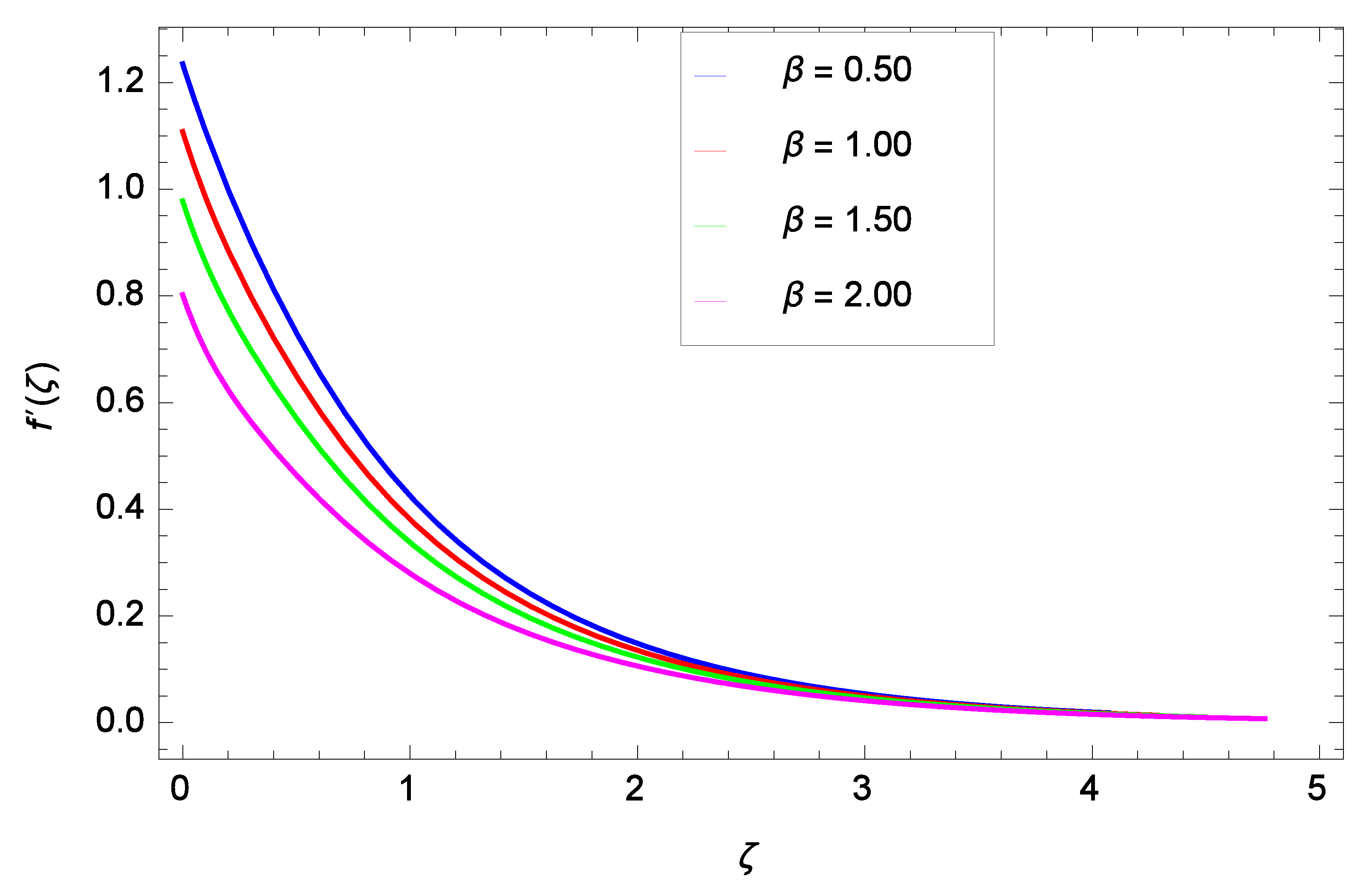
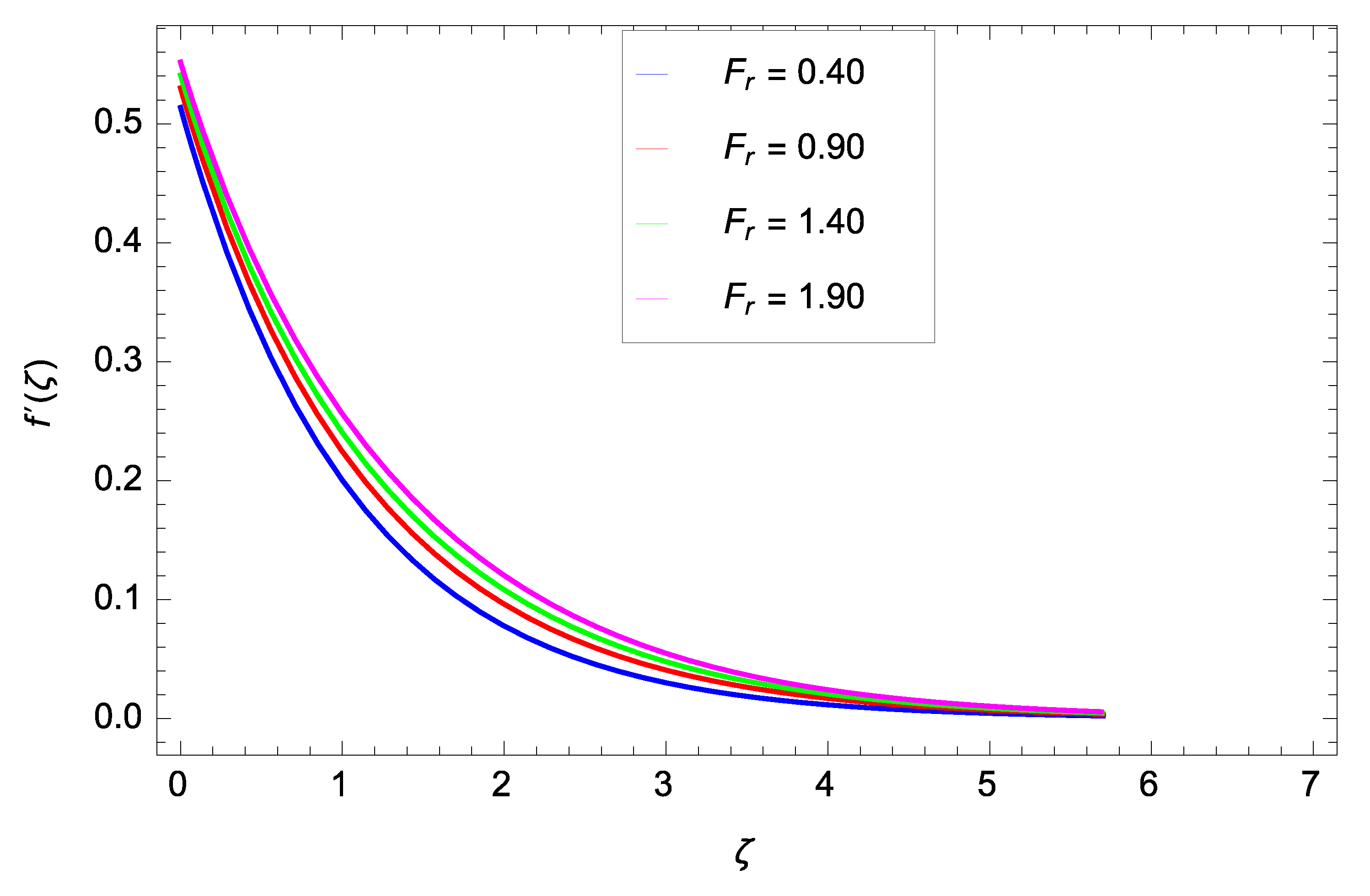
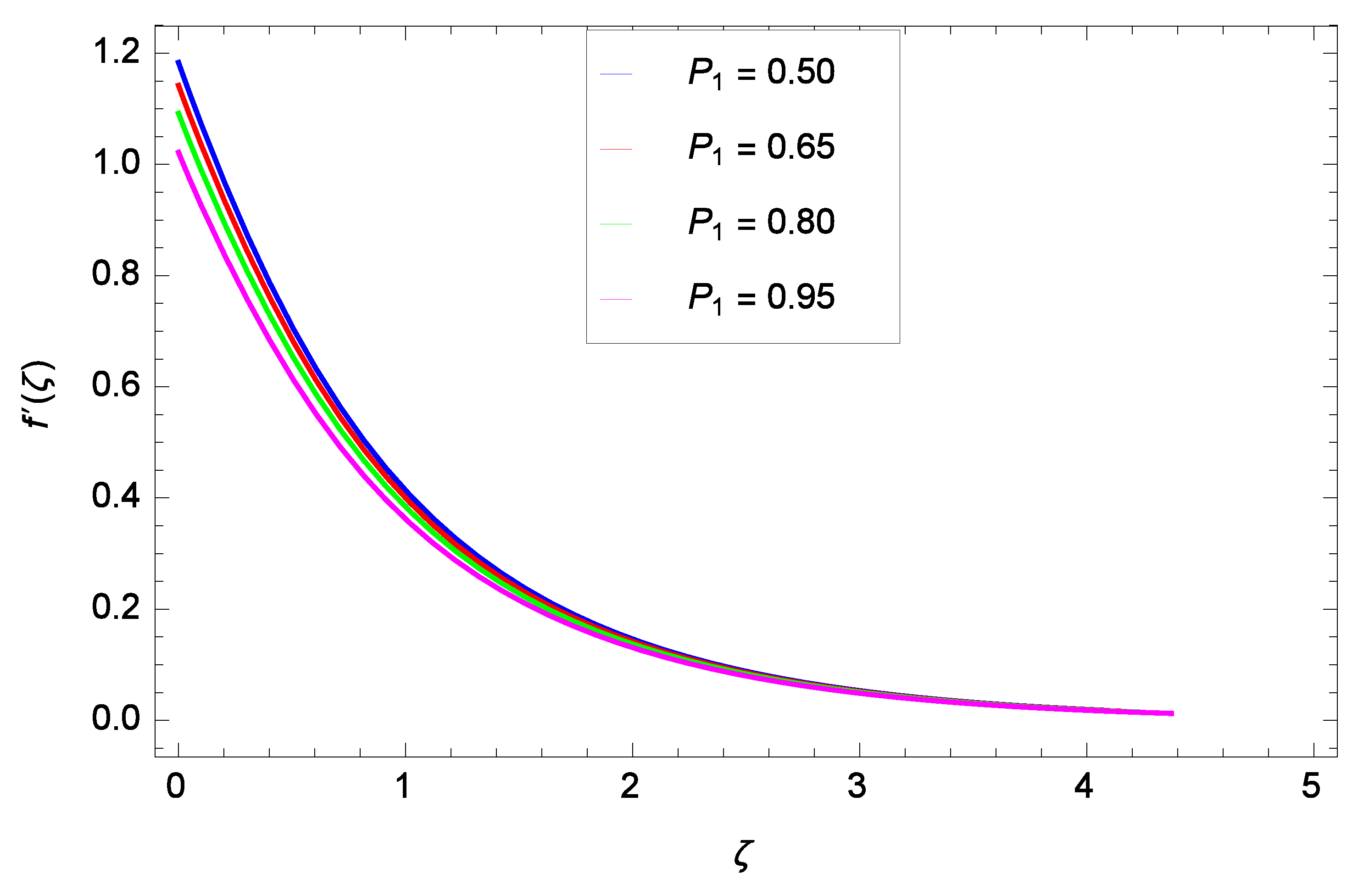
• The velocity decreases as the ferromagnetic interaction parameter, porosity parameter, and local inertia parameter increase.
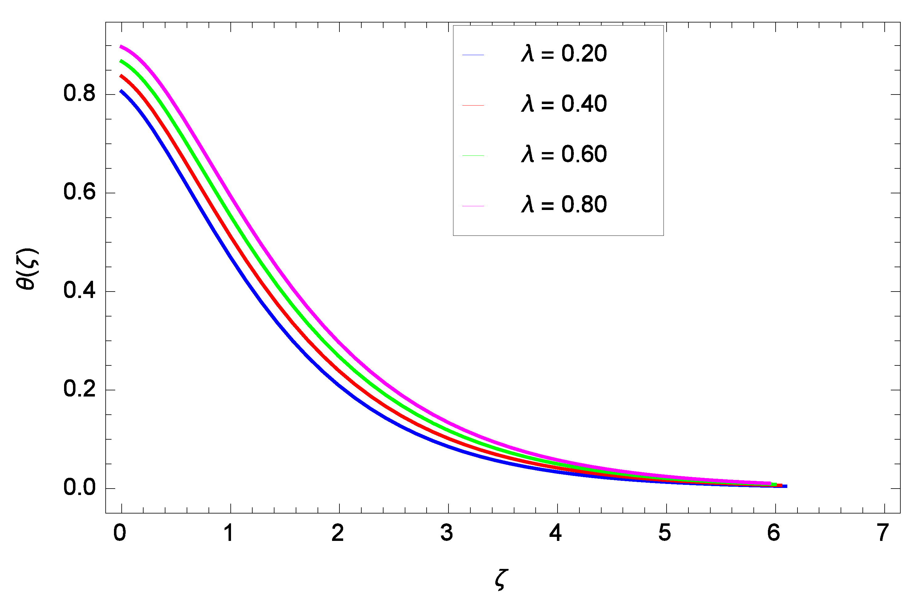
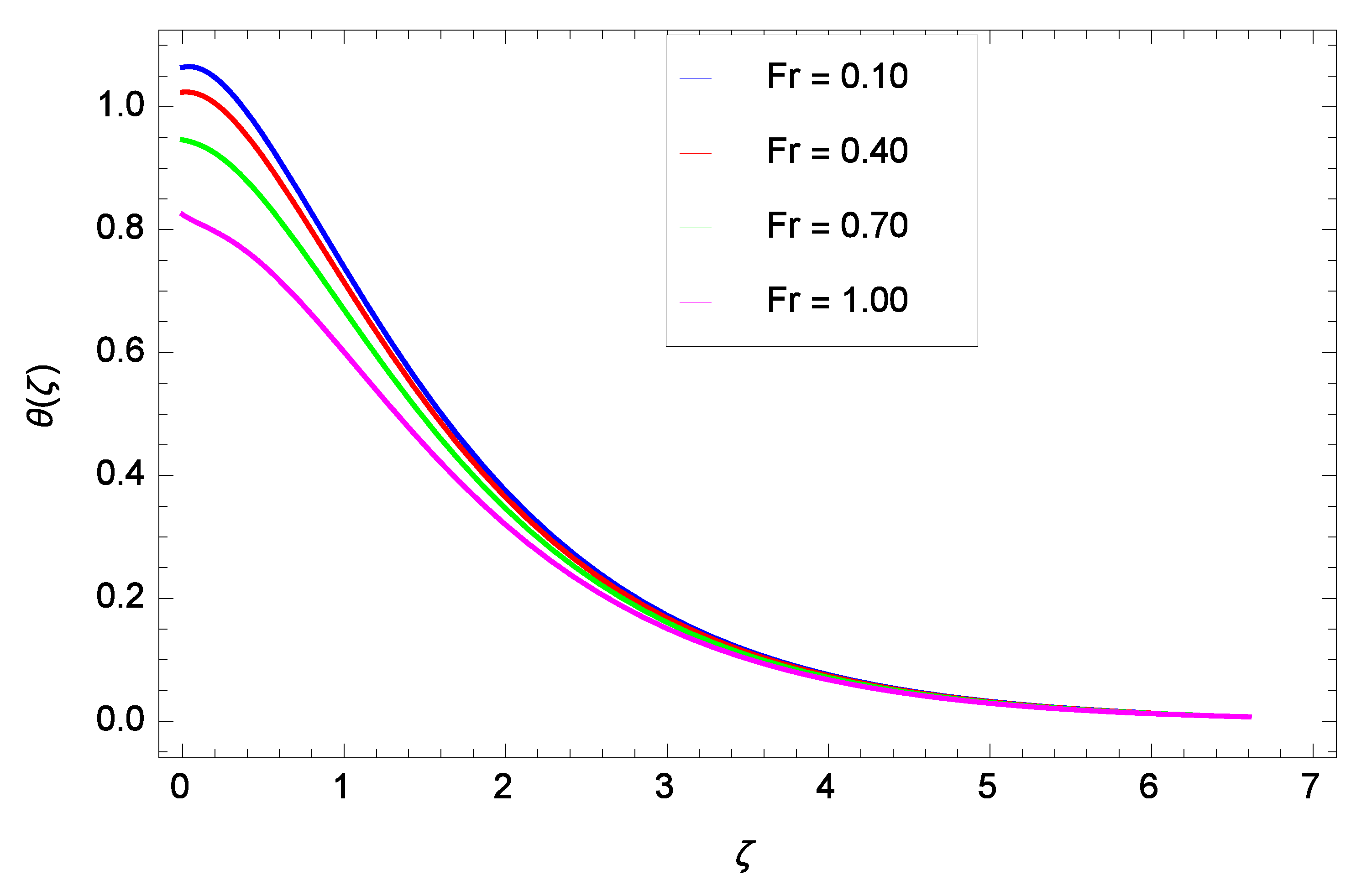
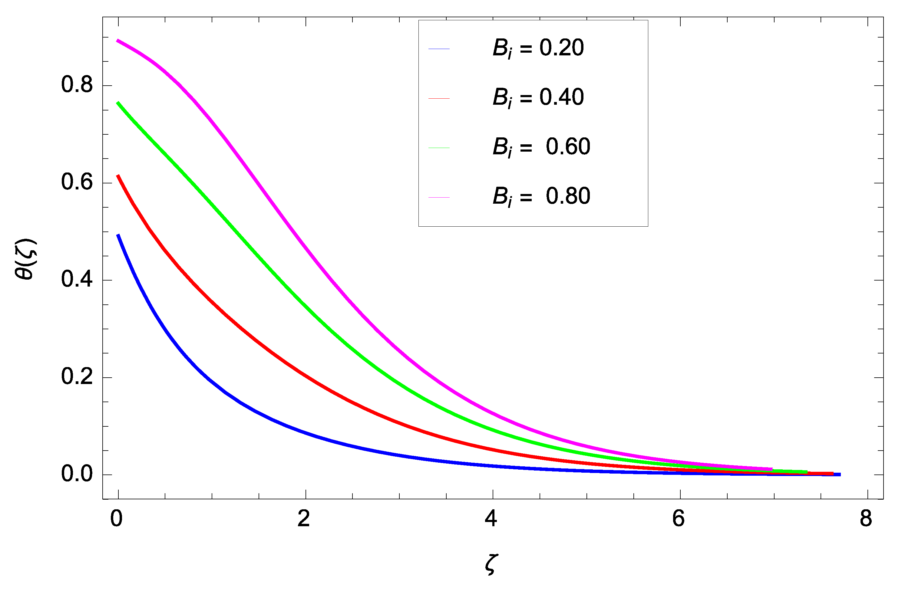
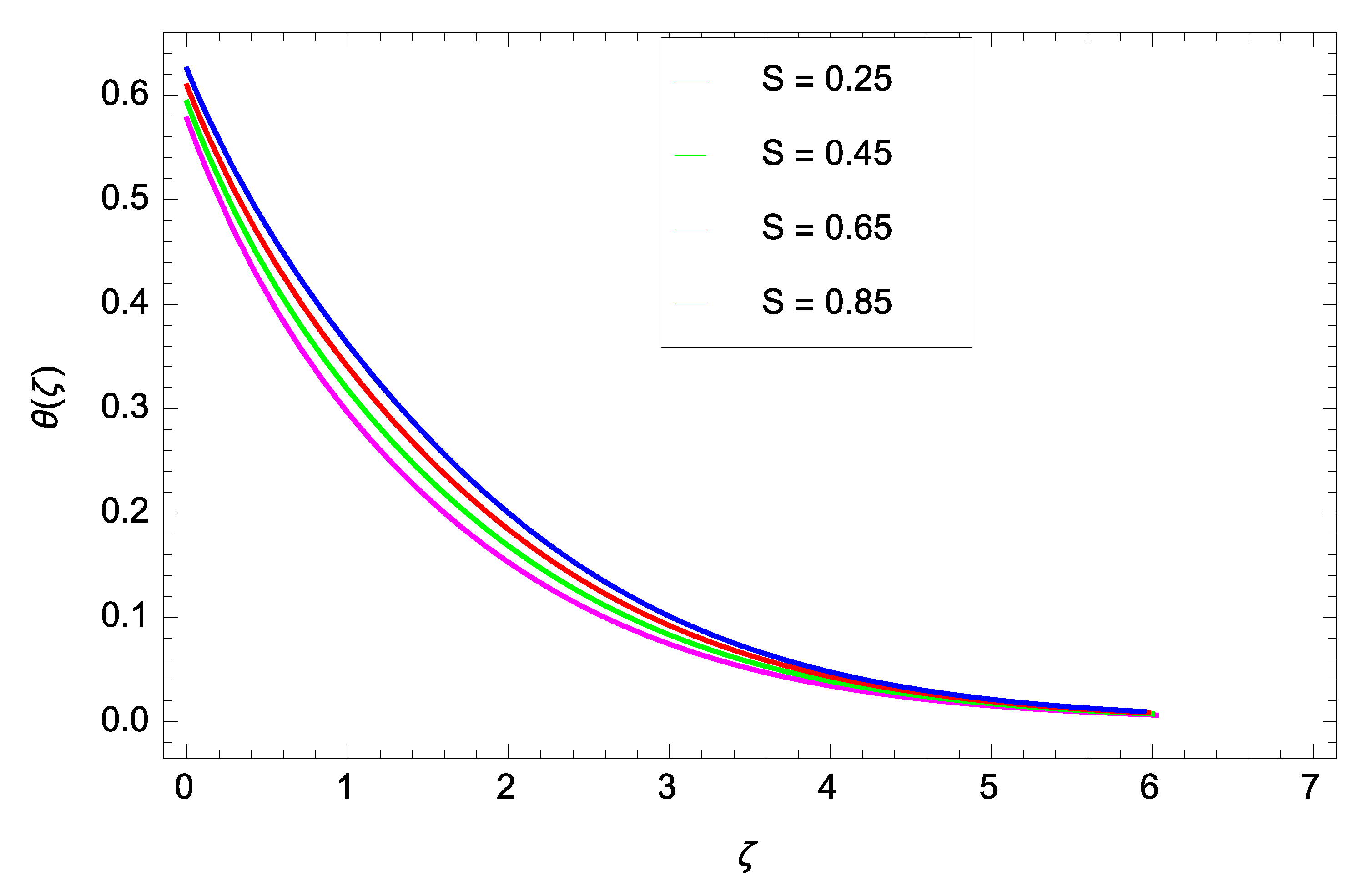
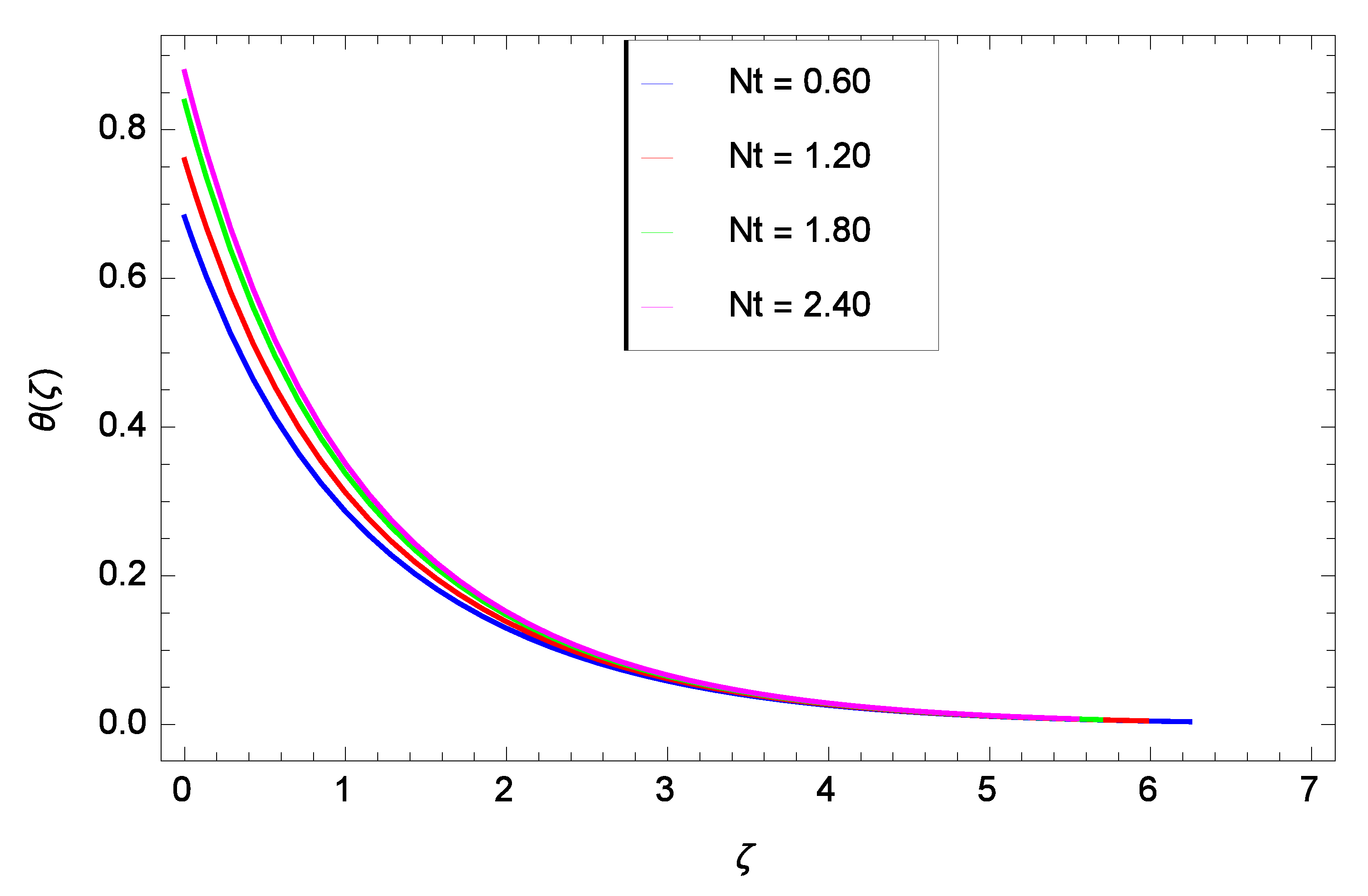
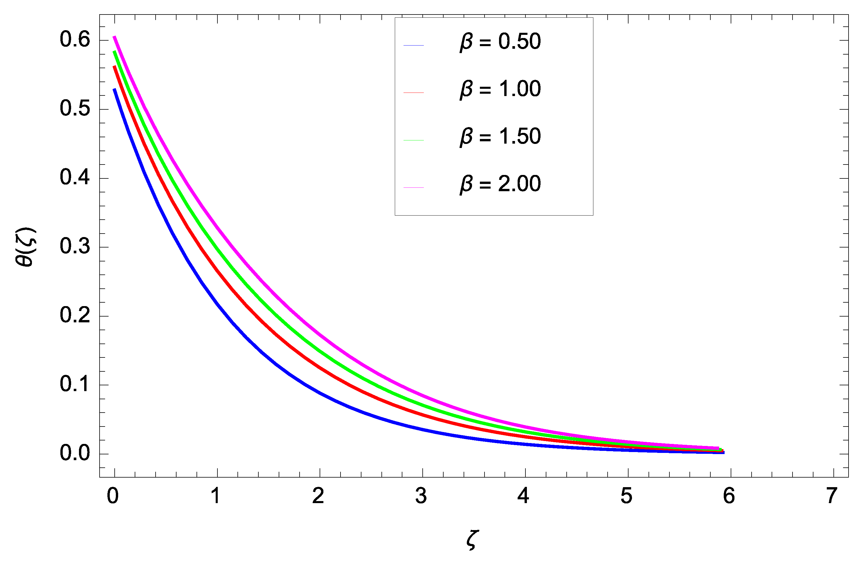
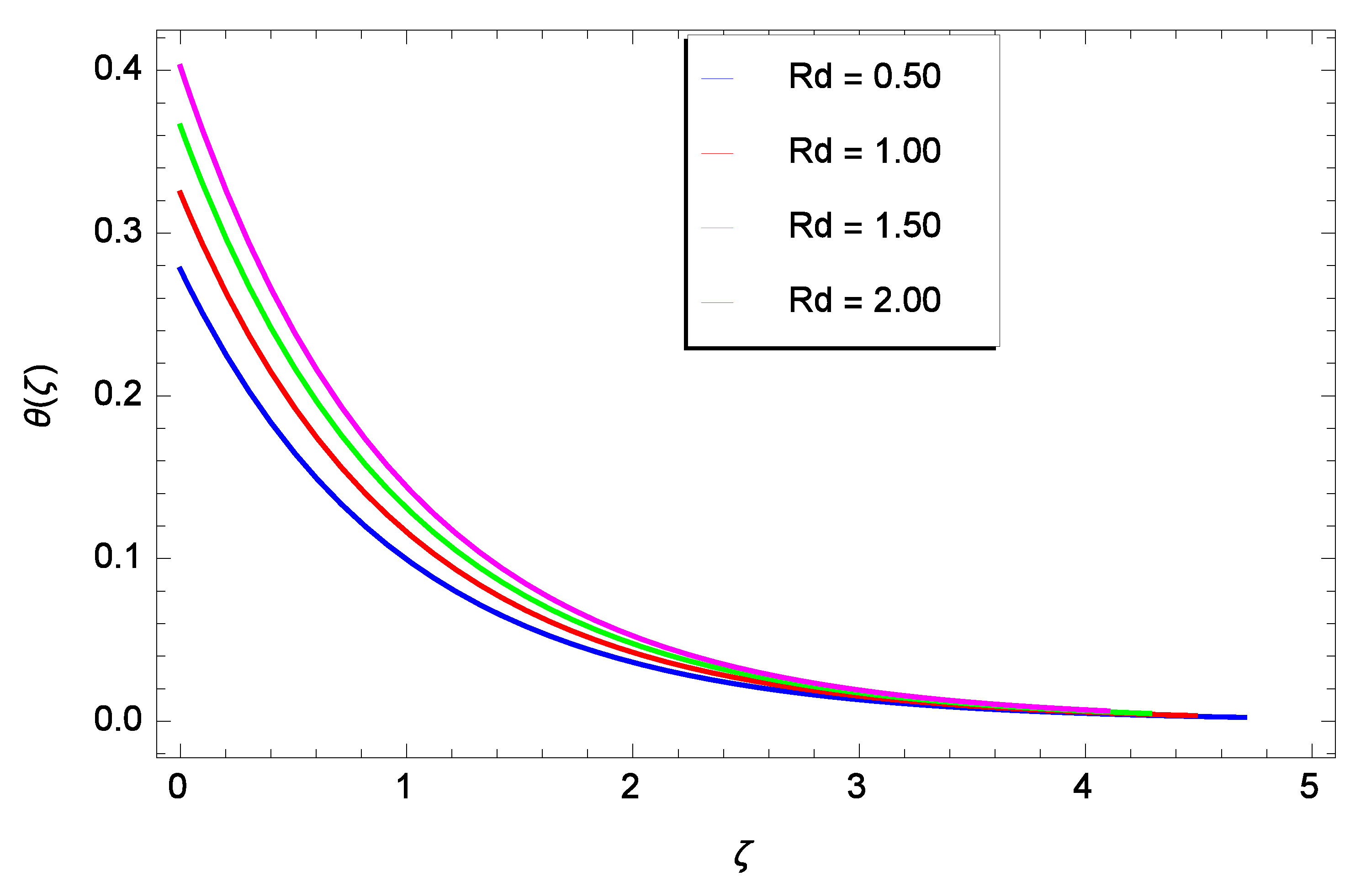
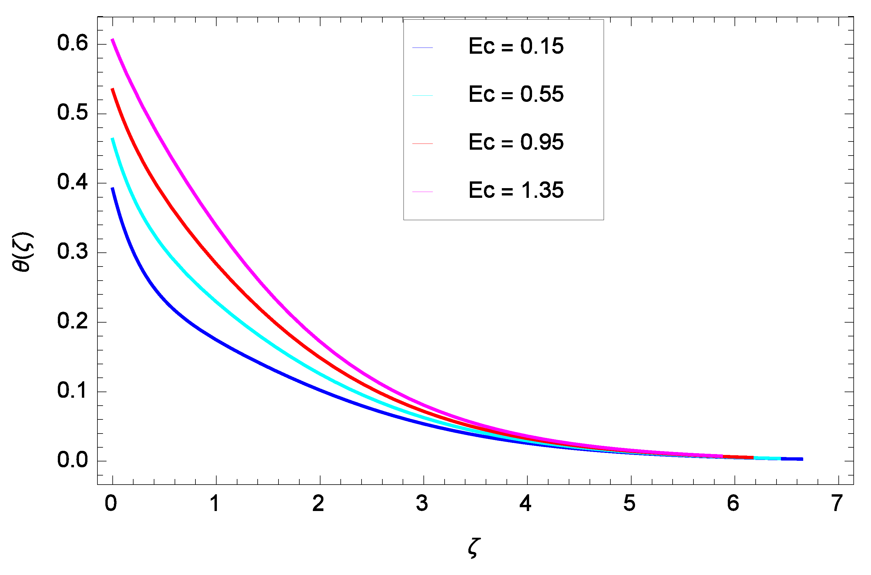
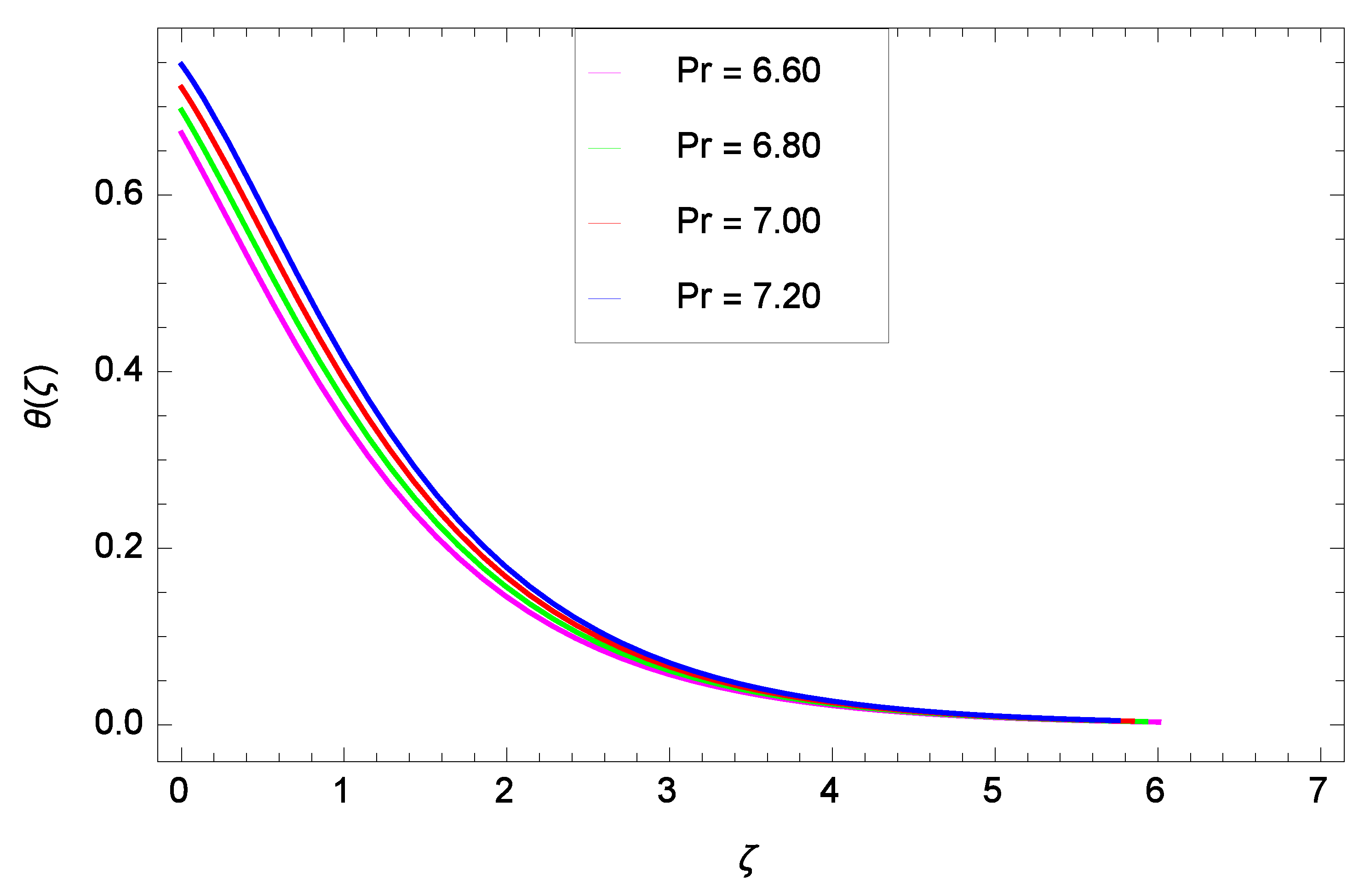
• The temperature rises as the ferromagnetic interaction, heat dissipation, injection, thermal radiation parameters and Eckert number are raised, and reduces when the Prandtl number and sunction parameter are raised.
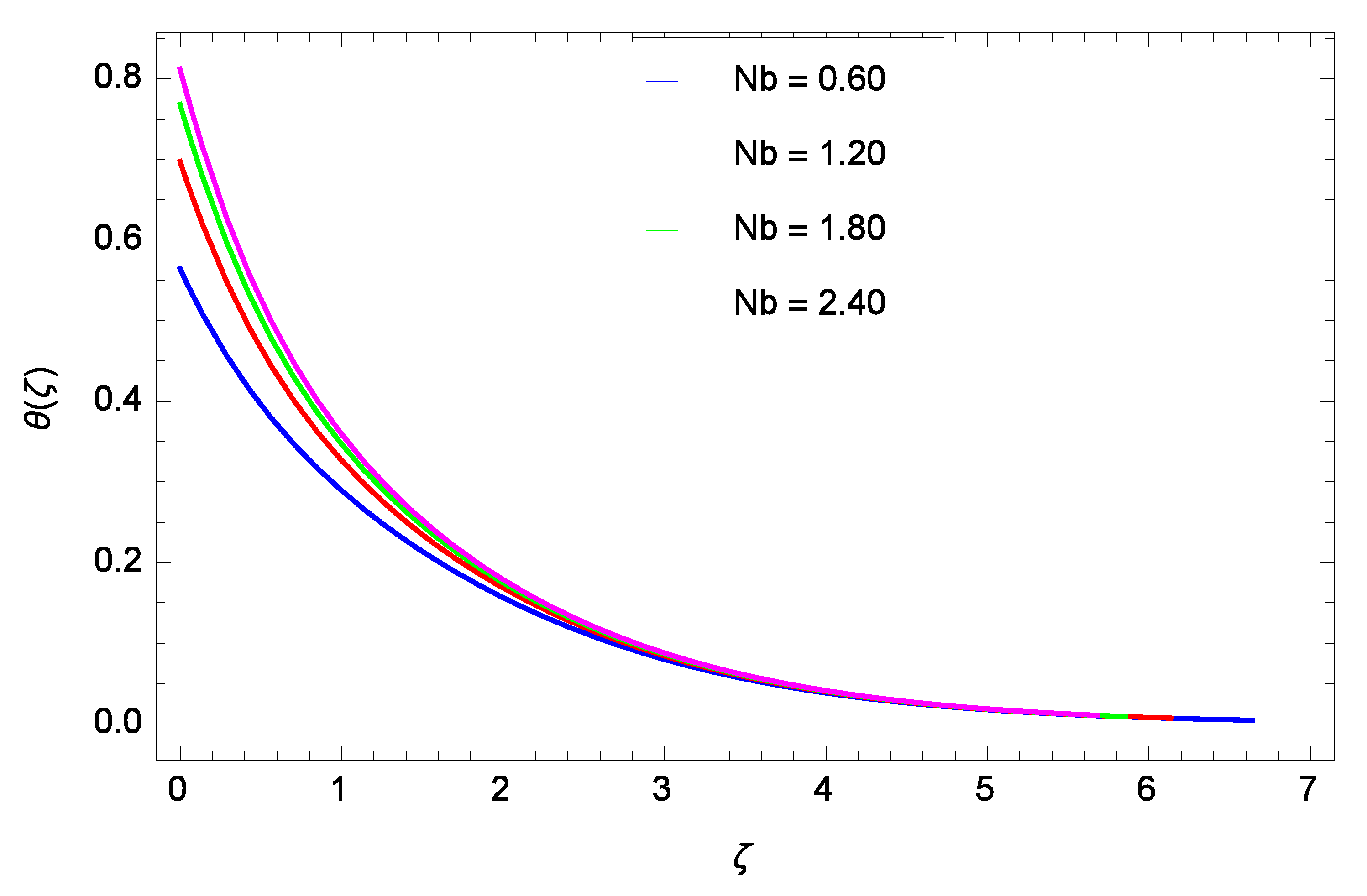
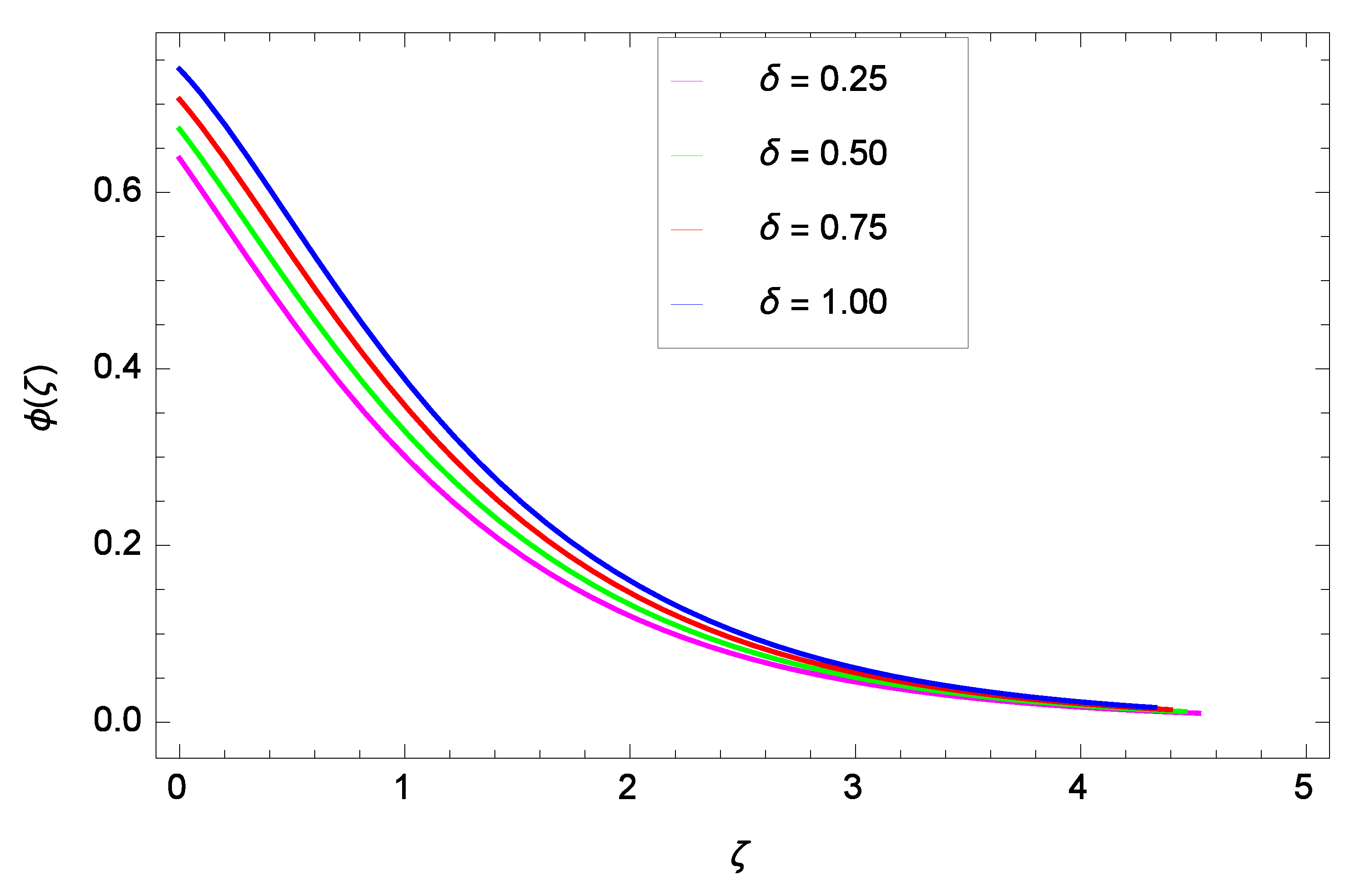
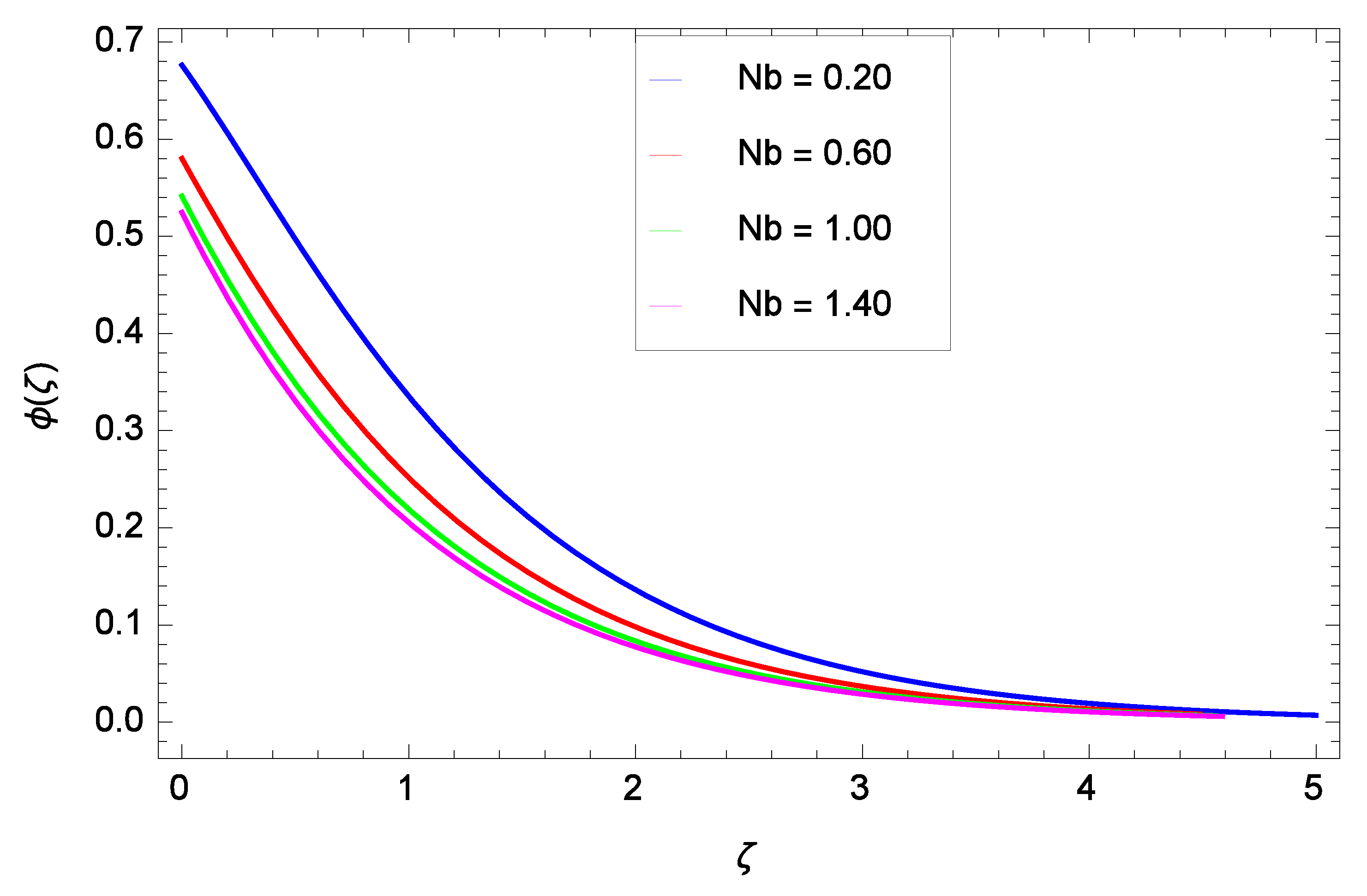
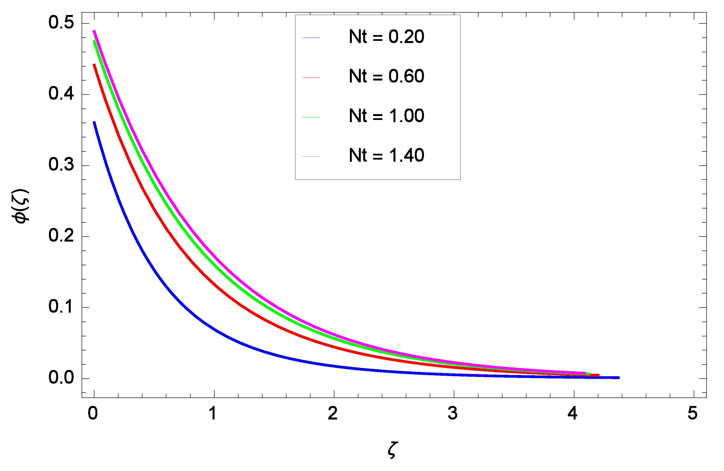
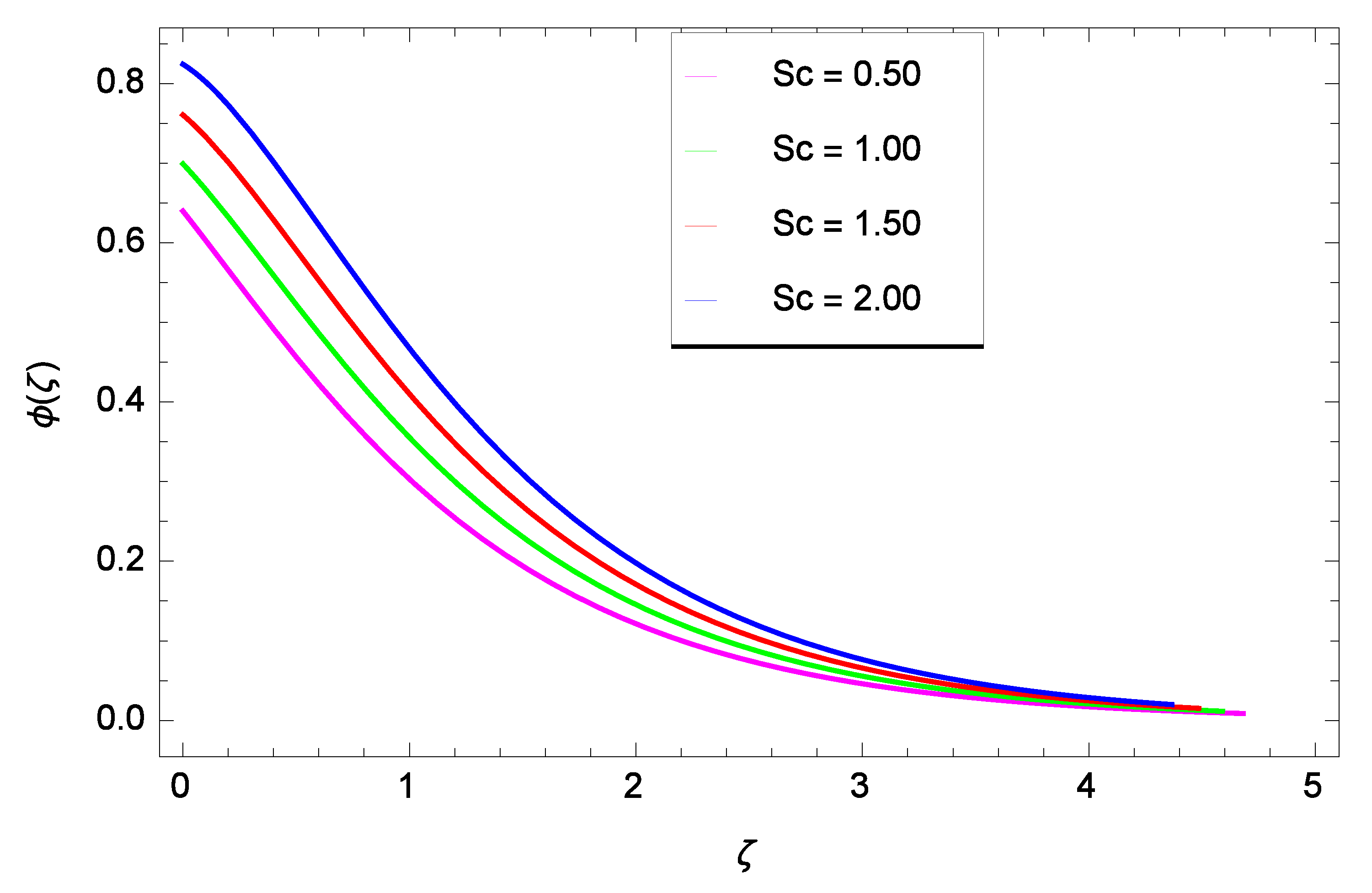
• When the Brownian motion, chemical reaction parameters and Schmidt number increase, the concentration decreases, while it increases when the thermophoresis parameter increases.
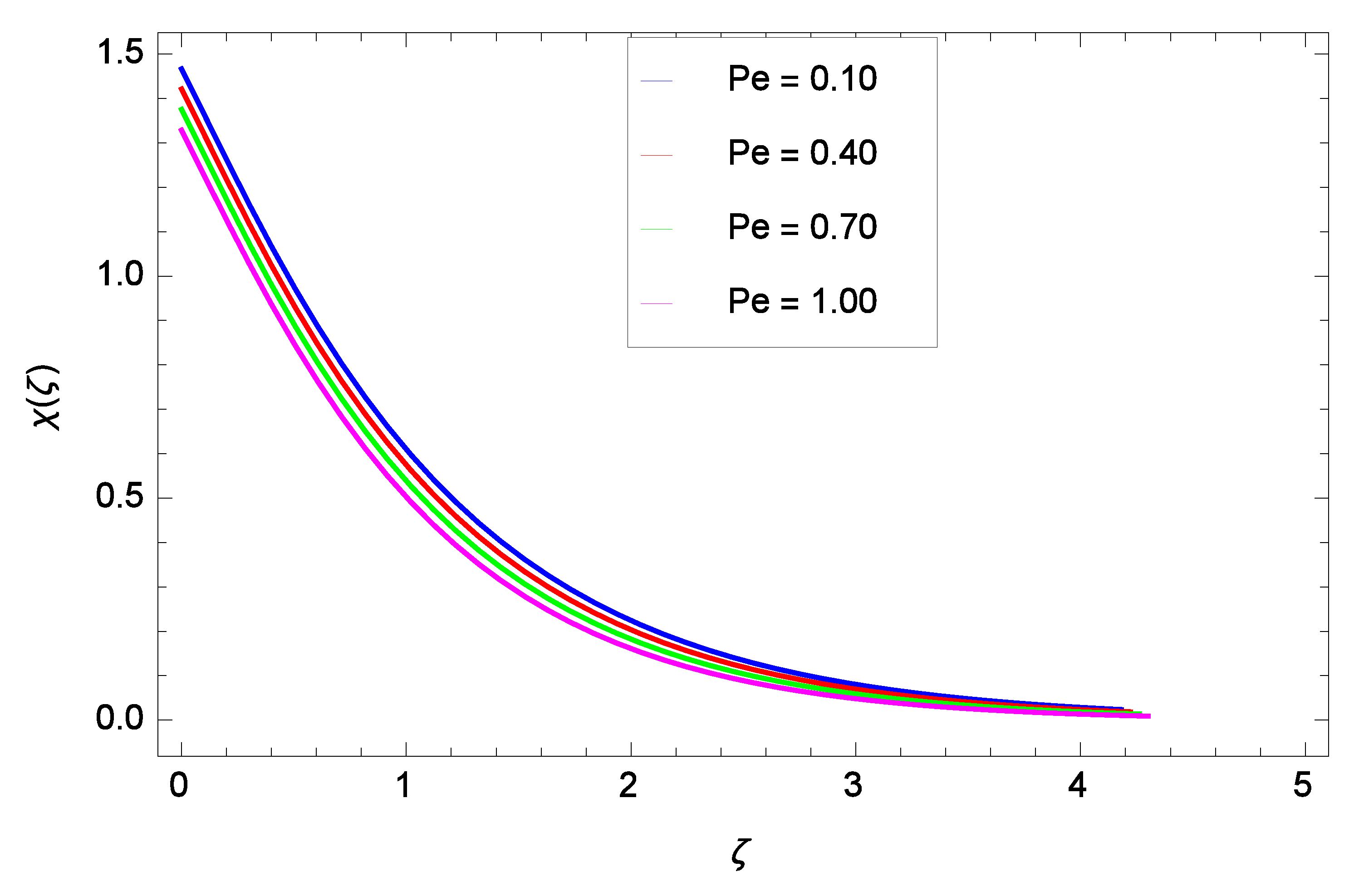
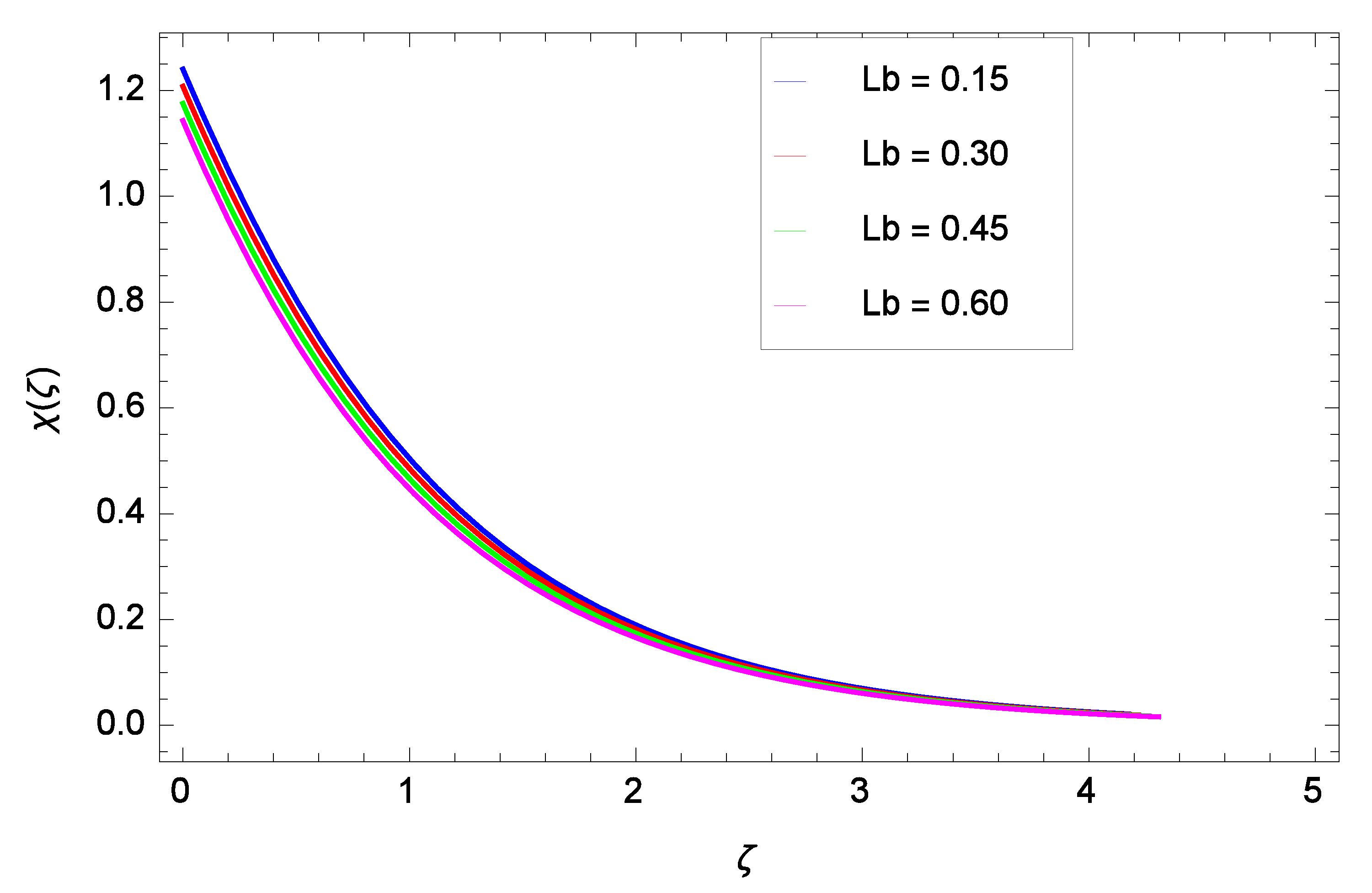
• The motile microorganism density decreases through raising the Peclet number and bioconvection Lewis number.

References

1. Raj, K.; Moskowitz, R. Commercial applications of ferrofluids. J. Magn. Magn. Mater. 1990, 85, 233–245. [Google Scholar] [CrossRef]
2. Goldman, A. Handbook of Modern Ferromagnetic Materials; Springer Science and Business Media: Berlin, Germany, 2012. [Google Scholar]
3. Hathway, D.B. dB-sound. Eng. Mag. 1979, 13, 42–44. [Google Scholar]
4. Andersson, H.I.; Valnes, O.A. Flow of a heated ferrofluid over a stretching sheet in the presence of a magnetic dipole. Acta Mech. 1998, 128, 39–47. [Google Scholar] [CrossRef]
5. Zeeshan, A.; Majeed, A.; Ellahi, R.; Zia, Q.M.Z. Mixed convection flow and heat transfer in ferromagnetic fluid over a stretching sheet with partial slip effects. Therm. Sci. 2018, 22, 2515–2526. [Google Scholar] [CrossRef]
6. Hayat, T.; Ahmad, S.; Khan, M.I.; Alsaedi, A. Exploring magnetic dipole contribution on radiative flow of ferromagnetic Williamson fluid. Results Phys. 2018, 8, 545–551. [Google Scholar] [CrossRef]
7. Choi, S.U.; Eastman, J.A. Enhancing Thermal Conductivity of Fluids with Nanoparticles; Argonne National Lab: Lemont, IL, USA, 1995.
8. Ellahi, R. The effects of MHD and temperature dependent viscosity on the flow of non-Newtonian nanofluid in a pipe: Analytical solutions. Appl. Math. Model. 2013, 37, 1451–1467. [Google Scholar] [CrossRef]
9. Ellahi, R.; Raza, M.; Akbar, N.S. Study of peristaltic flow of nanofluid with entropy generation in a porous medium. J. Porous Media 2017, 20, 461–478. [Google Scholar] [CrossRef]
10. Hayat, T.; Ahmad, S.; Khan, M.I.; Alsaedi, A. Modeling and analyzing flow of third grade nanofluid due to rotating stretchable disk with chemical reaction and heat source. Phys. B Condens. Matter. 2018, 537, 116–126. [Google Scholar] [CrossRef]
11. Awais, M.; Shah, Z.; Perveen, N.; Ali, A.; Kumam, P.; Thounthong, P. MHD effects on ciliary-induced peristaltic flow coatings with rheological hybrid nanofluid. Coatings 2020, 10, 186. [Google Scholar] [CrossRef] [Green Version]
12. Reddy, P.S.; Sreedevi, P.; Chamkha, A.J. MHD natural convection boundary layer flow of nanofluid over a vertical cone with chemical reaction and suction/injection. Comput. Therm. Sci. Int. J. 2017, 9, 165–182. [Google Scholar] [CrossRef]
13. Alsaedi, A.; Khan, M.I.; Farooq, M.; Gull, N.; Hayat, T. Magnetohydrodynamic (MHD) stratified bioconvective flow of nanofluid due to gyrotactic microorganisms. Adv. Powder Technol. 2017, 28, 288–298. [Google Scholar] [CrossRef]
14. Hayat, T.; Bashir, Z.; Qayyum, S.; Alsaedi, A. Nonlinear radiative flow of nanofluid in presence of gyrotactic microorganisms and magnetohydrodynamic. Int. J. Numer. Methods Heat Fluid Flow 2019, 29, 3039–3055. [Google Scholar] [CrossRef]
15. Nadeem, S.; Ijaz, M.; El-Kott, A.; Ayub, M. Rosseland analysis for ferromagnetic fluid in presence of gyrotactic microorganisms and magnetic dipole. Ain Shams Eng. J. 2020, 11, 1295–1308. [Google Scholar] [CrossRef]
16. Bhatti, M.M.; Michaelides, E.E. Study of Arrhenius activation energy on the thermo-bioconvection nanofluid flow over a Riga plate. J. Therm. Anal. Calorim. 2021, 143, 2029–2038. [Google Scholar] [CrossRef]
17. Waqas, H.; Khan, S.A.; Alghamdi, M.; Alqarni, M.S.; Muhammad, T. Numerical simulation for bio-convection flow of magnetized non-Newtonian nanofluid due to stretching cylinder/plate with swimming motile microorganisms. Eur. Phys. J. Spec. Top. 2021, 230, 1239–1256. [Google Scholar] [CrossRef]
18. Ingham, D.B.; Pop, I. (Eds.) Transport Phenomena in Porous Media III; Elsevier: Oxford, UK, 2005; Volume 3. [Google Scholar]
19. Zeng, Z.; Grigg, R. A criterion for non-Darcy flow in porous media. Transp. Porous Media 2006, 63, 57–69. [Google Scholar] [CrossRef]
20. Kumar, B.R.; Sivaraj, R. MHD viscoelastic fluid non-Darcy flow over a vertical cone and a flat plate. Int. Commun. Heat Mass Transf. 2013, 40, 1–6. [Google Scholar] [CrossRef]
21. Chamkha, A.; Abbasbandy, S.; Rashad, A.M. Non-Darcy natural convection flow for non-Newtonian nanofluid over cone saturated in porous medium with uniform heat and volume fraction fluxes. Int. J. Numer. Method Heat Fluid Flow 2015, 25, 422–437. [Google Scholar] [CrossRef]
22. Mallikarjuna, B.; Rashad, A.M.; Hussein, A.K.; Raju, S.H. Transpiration and thermophoresis effects on Non-Darcy convective flow past a rotating cone with thermal radiation. Arab. J. Sci. Eng. 2016, 41, 4691–4700. [Google Scholar] [CrossRef]
23. Durairaj, M.; Ramachandran, S.; Mehdi, R.M. Heat generating/absorbing and chemically reacting Casson fluid flow over a vertical cone and flat plate saturated with non-Darcy porous medium. Int. J. Numer. Method Heat Fluid Flow 2017, 27, 156–173. [Google Scholar] [CrossRef]
24. Pătrulescu, F.O.; Groşan, T.; Pop, I. Natural convection from a vertical plate embedded in a non-Darcy bidisperse porous medium. J. Heat Transf. 2020, 142, 012504. [Google Scholar] [CrossRef]
25. Liao, S.J. The Proposed Homotopy Analysis Method for the Solution of Nonlinear Problems. Ph.D. Thesis, Shanghai Jiao Tong University, Shanghai, China, 1992. [Google Scholar]
26. Liao, S.J. An explicit, totally analytic approximate solution for Blasius viscous flow problems. Int. J. Non-Linear Mech. 1999, 34, 759–778. [Google Scholar] [CrossRef]
27. Liao, S. Beyond Perturbation: Introduction to the Homotopy Analysis Method; CRC Press: Boca Raton, FL, USA, 2003. [Google Scholar]
28. Irfan, M.; Khan, M.; Khan, W.A.; Sajid, M. Thermal and solutal stratifications in flow of Oldroyd-B nanofluid with variable conductivity. Appl. Phys. A 2018, 124, 674. [Google Scholar] [CrossRef]
29. Tlili, I.; Waqas, H.; Almaneea, A.; Khan, S.U.; Imran, M. Activation energy and second order slip in bioconvection of Oldroyd-B nanofluid over a stretching cylinder: A proposed mathematical model. Processes 2019, 7, 914. [Google Scholar] [CrossRef] [Green Version]
30. Usman, A.H.; Khan, N.S.; Humphries, U.W.; Ullah, Z.; Shah, Q.; Kumam, P.; Thounthong, P.; Khan, W.; Kaewkhao, A.; Bhaumik, A. Computational optimization for the deposition of bioconvection thin Oldroyd-B nanofluid with entropy generation. Sci. Rep. 2021, 11, 11641. [Google Scholar] [CrossRef] [PubMed]
31. Hayat, T.; Waqas, M.; Shehzad, S.A.; Alsaedi, A. Mixed convection flow of viscoelastic nanofluid by a cylinder with variable thermal conductivity and heat source/sink. Int. J. Numer. Method Heat Fluid Flow 2016, 26, 214–234. [Google Scholar] [CrossRef]
Figure 1. A picture scheme of the problem.
Coatings 11 01129 g001
Figure 2. Influence of β on f ( ζ ) .
Coatings 11 01129 g002
Figure 3. Influence of F r on f ( ζ ) .
Coatings 11 01129 g003
Figure 4. Influence of P 1 on f ( ζ ) .
Coatings 11 01129 g004
Figure 5. Influence of R a b on f ( ζ ) .
Coatings 11 01129 g005
Figure 6. Influence of β on θ ( ζ ) .
Coatings 11 01129 g006
Figure 7. Influence of λ on θ ( ζ ) .
Coatings 11 01129 g007
Figure 8. Influence of F r on θ ( ζ ) .
Coatings 11 01129 g008
Figure 9. Influence of B i on θ ( ζ ) .
Coatings 11 01129 g009
Figure 10. Influence of S < 0 on θ ( ζ ) .
Coatings 11 01129 g010
Figure 11. Influence of S > 0 on θ ( ζ ) .
Coatings 11 01129 g011
Figure 12. Influence of R d on θ ( ζ ) .
Coatings 11 01129 g012
Figure 13. Influence of N t on θ ( ζ ) .
Coatings 11 01129 g013
Figure 14. Influence of N b on θ ( ζ ) .
Coatings 11 01129 g014
Figure 15. Influence of E c on θ ( ζ ) .
Coatings 11 01129 g015
Figure 16. Influence of P r on θ ( ζ ) .
Coatings 11 01129 g016
Figure 17. Influence of δ on ϕ ( ζ ) .
Coatings 11 01129 g017
Figure 18. Influence of N b on ϕ ( ζ ) .
Coatings 11 01129 g018
Figure 19. Influence of N t on ϕ ( ζ ) .
Coatings 11 01129 g019
Figure 20. Influence of S c on ϕ ( ζ ) .
Coatings 11 01129 g020
Figure 21. Influence of P e on χ ( ζ ) .
Coatings 11 01129 g021
Figure 22. Influence of L b on χ ( ζ ) .
Coatings 11 01129 g022