Enhanced Anti-Corrosion Performances of Epoxy Resin Using the Addition of Sodium Dodecylbenzene Sulfonate-Modified Graphene

Abstract

The improvement of anti-corrosive property of epoxy resin is significant for the development of coatings to avoid metal corrosion and thus to reduce the economic loss in many industries. The superior properties of graphene, a two-dimensional material, make it possibly suitable to fulfill this task. However, this is hindered by the easy agglomeration of graphene layers in solvents. In the present work, we report the modification and stabilization of graphene in water using sodium dodecylbenzene sulfonate (SDBS) and the enhancement of the anti-corrosive properties of epoxy resin by mixing such SDBS-modified graphene layers. The influence of the dosage of SDBS on the modification effect of graphene was studied in detail and an optimized dosage, i.e., 50 mg SDBS for 10 mg graphene, was obtained. The SDBS modification could effectively reduce graphene thickness, and the minimum thickness of the modified graphene was 3.50 nm. The modified graphene had increased layer spacing, and the maximum layer spacing was 0.426 nm. When the modified graphene was added into the epoxy resin, the electrochemical impedance modulus value evidently increased compared to pure epoxy resin and those incorporated by pure graphene, indicating that the anti-corrosion performance was significantly improved. These results clarified that SDBS could effectively modify graphene and the SDBS-modified graphene could subsequently largely improve the anti-corrosive property of epoxy resin, which is of significance for the anti-corrosive coatings.

1. Introduction

Metal corrosion recently being increasing economic loss, many efforts have been made to prevent corrosion of metals or minimize the metal corrosion rate. Various methods including improving the substrate, covering the protective layer, electrochemical protection, etc. have been developed [1,2]. Anti-corrosive coating is a very economical and effective method for metal protection [3]. Among the coatings materials available, epoxy resin-based coatings are one of the most widely used ones for various applications. Therefore, it is of great interest to improve the corrosive performance of epoxy resin. Graphene, as a typical two-dimensional material, has been proved to be helpful for this purpose due to its excellent barrier property and high conductivity [4,5,6,7]. For instance, Chen et al. [8] used 2-Dibutylaniline (P₂BA) to modify graphene in tetrahydrofuran solvent, and mixed the modified graphene (P₂BA-G) into epoxy resin E44, and further, this E44 was coated on the Q235 steel plate for testing. The results show that the anti-corrosion performance of epoxy resin E44 is significantly improved. Ramezanzadeh et al. [9] used p-phenylenediamine to modify graphene oxide and transferred the modified graphene oxide to epoxy resin by a wet process to prepare modified graphene/epoxy resin composites. In addition, the prepared composite material was coated on low carbon steel for electrochemical test. The results showed that the anti-corrosion performance of composite materials with 0.1% mass ratio of modified graphene was significantly improved. Dou et al. [10] found that the addition of fluorinated graphene sheet to waterborne epoxy resin (WEP) can not only significantly improve the tensile strength of the WEP coating but also increase its barrier properties. The graphene sheet helps block the penetration of corrosive agent throughout the coating to the interface between coating and substrate. There are two main reasons why graphene can improve the performance of anti-corrosion coating. (1) The ‘stacking’ of sheet structure graphene. The ‘stacking’ of graphene can play a barrier effect in water, gas, corrosive substances, etc. (2) Graphene sheets are hydrophobic materials, and a few layers of graphene (mainly 3–5 layers) are more hydrophobic, which leads to a physical anti-corrosion effect [11].

When incorporating graphene into coatings, the biggest challenge is the easy agglomeration of graphene, which is mainly induced by the bonding of the dangling bonds on the surface of graphene [12]. The aggregation of graphene forms holes in the coating, which provides a way for the corrosive medium to reach the substrate and accelerate the corrosion. This leads eventually to the invalidation of anti-corrosion. Therefore, it is of great importance to modify graphene. Graphene modification includes covalent bond modification and non-covalent modification. Li et al. [11] reported the example of non-covalent bond modification of graphene nanosheets using poly(sodium styrene sulfonate) (PSS), and the addition of modified graphene can significantly improve the anti-corrosion performance of epoxy zinc containing anti-corrosion coating. Covalent bond modification is more stable and effective; covalent modification refers to the substitution reaction of the modified substance with oxygen-containing groups on the surface of graphene or graphene oxide, mostly using graphene oxide, which contains a reduction reaction process and thus more defects in graphene [13]. Yao et al. [14] prepared homogeneous dispersion of graphene nanosheets in epoxy via chemical functionalization of graphene oxide with 4-nitrobenzenediazonium salt in the presence of sodium dodecyl benzene sulfonate (SDBS) and compared it with neat epoxy: the tensile strength and elongation at break of epoxy nanocomposites were increased. However, SDBS was only used as a surfactant when 4-nitrobenzenediazonium salt modified graphene oxide and when the manufacturing process of first modifying graphene oxide and then reducing it is more complex. Moreover, the systematic study on the anti-corrosion performance of the modified epoxy resin is still lacking.

In this work, graphene was directly modified by different content of SDBS and well-dispersed graphene dispersion was obtained by ultrasonication. It is well known that ultrasonication could effectively enhance the graphene dispersion [15]. Raman spectroscopy, atomic force microscopy (AFM), and X-ray diffraction (XRD) show that graphene has excellent properties such as 2–3 layers feature, large area, and low defects. The electrochemical impedance spectroscopy test of epoxy resin samples with different immersion times shows that the addition of graphene modified by SDBS can effectively improve the corrosion resistance of epoxy resin.

2. Experimental

2.1. Materials

Graphene was purchased from Nanjing XFNANO Materials Tech Co., Ltd. (Nanjing, China). SDBS powder was obtained from Sinopharm Group Chemical Reagent Co., Ltd. (Shanghai, China). Curing agent was obtained from Shanxi Baotashan Paint Co., Ltd. (Xi’an, China). Epoxy resin solution (EP20 60%) was obtained from Shanxi Baotashan Paint Co., Ltd. (Xi’an, China).

2.2. Preparation of Modified Graphene

Graphene and SDBS powder were weighted as a certain mass ratio (SDBS/graphene,

Table 1. The composition of modified graphene samples.

	Sample Number	G	G-1S	G-5S	G-10S	G-20S
Materials
Graphene (mg)		10	10	10	10	10
SDBS (mg)		0	10	50	100	200
SDBS/graphene weight ratio		0	1	5	10	20

) and deionized water was mixed with a mass ratio of 1:1000 (graphene/deionized water); the mixed solution was then magnetically stirred. The speed of the magnetic stirrer (Shanghai sile Instrument Co., Ltd., Shanghai, China) was 700 rounds per minute (rpm) and the time was 5 min to obtain the modified graphene dispersion. Then, the graphene dispersion was treated by ultrasonic cleaning instrument; the ultrasonic treatment process includes two steps. First, the sample was ultrasonicated with high power of 600 W for 30 min, followed with ultrasonic treatment with low power of 120 W for 60 min. Finally, a stable modified graphene dispersion was obtained.

The components of different samples are shown in Table 1.

2.3. Preparation of Graphene-Modified Epoxy Resin

We used sample G-5S (chemical composition shown in Table 1) for the study. A certain amount (as shown in

Table 2. Composition of graphene-modified epoxy resin samples.

	Sample Number	E	ES	EG0.1	ESG0.1	EG0.5	ESG0.5
Materials
60%EP20 (g)		10	10	10	10	10	10
Curing agent (g)		1	1	1	1	1	1
Graphene (mg)		0	0	10	10	50	50
SDBS (mg)		0	50	50	50	250	250
Graphene (weight%)		0	0	0.1%	0.1%	0.5%	0.5%

) of 60% EP20 solution was mixed with the modified graphene dispersion (as shown in Table 2) and then stirred for 3 min to make the graphene fully dispersed. After uniformly stirring, the mixture was centrifuged at a speed of 3000 rpm for 15 min, and then, the supernatant was aspirated with a needle and discarded. EP20 curing agent was added into the centrifuge tube, according to the mass ratio in Table 2, stirred for 3 min, and kept still for further 5 min. The Q235 steel plates surface was polished with 400/600/800/1000 mesh sandpaper, washed with acetone and alcohol for 10 min, and then dried with a clean dust-free paper. The prepared epoxy coating was coated on the steel plate with wire rods. After a natural air drying for 36 h, the coating with thickness of about 20 µm was obtained. The components of the prepared graphene-modified epoxy resin samples are shown in Table 2.

2.4. Characterization

Raman spectra were measured with a HORIBA LabRAM HR Evolution spectrometer (HORIBA, Paris, France) using a laser wavelength of 532 nm to characterize the properties of modified graphene samples with different components. Atomic force microscopy (AFM, Dimension Icon-Bruker, billerica, MA, USA) was performed to observe the morphology of the modified graphene and to characterize the thickness of modified graphene samples. Infrared spectra were measured with Nicolet iS50 from Thermo Scientific (Waltham, MA, USA). The sample powder and the dry KBr powder were mixed with the mass ratio of 1:50 (sample/KBr). The X-ray diffraction was performed using an X-ray diffractometer from PANalytical company (Almero, The Netherlands) with a monochromated Cu Kα1 radiation source. The electrochemical corrosion test was performed in 3.5% NaCl solution on a PARSTAT MS electrochemical workstation (Princeton, NJ, USA). The Tafel polarization curves and electrochemical impedance spectroscopy were acquired by a classical three-electrode system at room temperature with a platinum (Pt) plate, a saturated calomel electrode (SCE), and the coating/Q235 steel as counter electrode, reference electrode, and working electrode, respectively.

3. Results and Discussion

The molecular structure of SDBS is shown in Figure 1. The dispersion in deionized (DI) water of the modified graphene sheets was studied. The photos of the modified graphene samples with different proportions (pure G, G-1S, G-5S, G-10S, and G-20S) after 1 h of standing are shown in Figure 2a–e, respectively. It can be seen from Figure 2 that the sample G is agglomerated, the graphene is black, and the solution itself is transparent, while the samples G-1S, G-5S, G-10S, and G-20S can be stably dispersed in DI water after 1 h of standing.

To get the insights of the graphene quality of the samples, Raman spectroscopy was carried out. Figure 3a shows Raman spectra of all graphene samples. For the pure graphene (black curve, G), it can be seen that three characteristic peaks arise at 1356, 1582, and 2724 cm⁻¹, which correspond to D, G, and 2D bands, respectively. The G peak is due to the in-plane bonding and contraction of carbon atoms in the sp² orbital hybridization, indicating the symmetry and ordering of the reaction materials [16]. The D peak represents the structural defects or edges of graphene [17]. Generally, the shape and position of 2D peak can be used to judge whether graphene is single-, double-, and multi-layered. The 2D peak of monolayer graphene is sharp, and with the increase in graphene layers, the shoulder of 2D peak is more obvious and the peak position moves to higher wave number [18].

Figure 3b shows the more detailed Raman spectra of graphene 2D peaks. As seen in Figure 3b, after incorporation of SDBS, the 2D peaks of all the samples shifted to lower wavenumbers, indicating decrease in the layers of the modified graphene [19], whereas the G-5S sample showed the largest 2D peak shift, i.e., from 2712.1 cm⁻¹ of pure graphene to 2718.3 cm⁻¹.

In order to examine the morphology and the thickness of the graphene samples, AFM measurements were performed. Figure 4 shows the AFM results of graphene samples. It can be seen from Figure 4a that in sample G, the unmodified graphene exhibits stripe-shaped wrinkles, which cannot be spread flat on the silicon wafer, and the maximum height extracted from the line profile analysis (Figure 4f) is 13.87 nm. In sample G-1S (Figure 4b), it can be clearly observed that the graphene forms flakes with uniform thickness. The extracted thickness is 4.71 nm (Figure 4f), which corresponds to 4 layers of graphene [1]. In sample G-5S (Figure 4c), the graphene is distributed in flakes with uniform thickness, and the extracted thickness of this sample is the lowest among all the samples. The extracted thickness is 3.50 nm (Figure 4f), which is about the thickness of 3 layers of graphene. The thickness of G-5S is smaller than that of G-10S (Figure 4d) and G-20S (Figure 4e), which is 4.12 and 4.15 nm, respectively (Figure 4f).

It is interesting to further understand the details of SDBS modification effect on graphene layers. Thus, Fourier infrared (FIR) spectra were investigated on all the samples. Figure 5a–c shows the FIR spectra of the samples G, SDBS, and G-5S, respectively. Due to the symmetry of the graphene structure, the pure G sample shows no clear characteristic FIR peak, as shown in Figure 5a. Figure 5b shows the FIR spectrum of the SDBS sample. The peaks at 2965, 2912, and 2853 cm⁻¹ are related to the vibration of the C−H bond in the SDBS. The peaks at 1132 and 1455 cm⁻¹ are produced by the vibration of CH₃, CH₂, and other bonds in SDBS; the peaks at 1633 and 3475 cm⁻¹ are induced by the vibration of −OH in water. Figure 5c shows the FIR spectrum of the sample G-5S; the peak position of the characteristic peak is almost the same as that of the modified substance SDBS sample. The FIR results show that the modified graphene sample powder contains SDBS, indicating that the modification of graphene is formed by the interaction between graphene and SDBS.

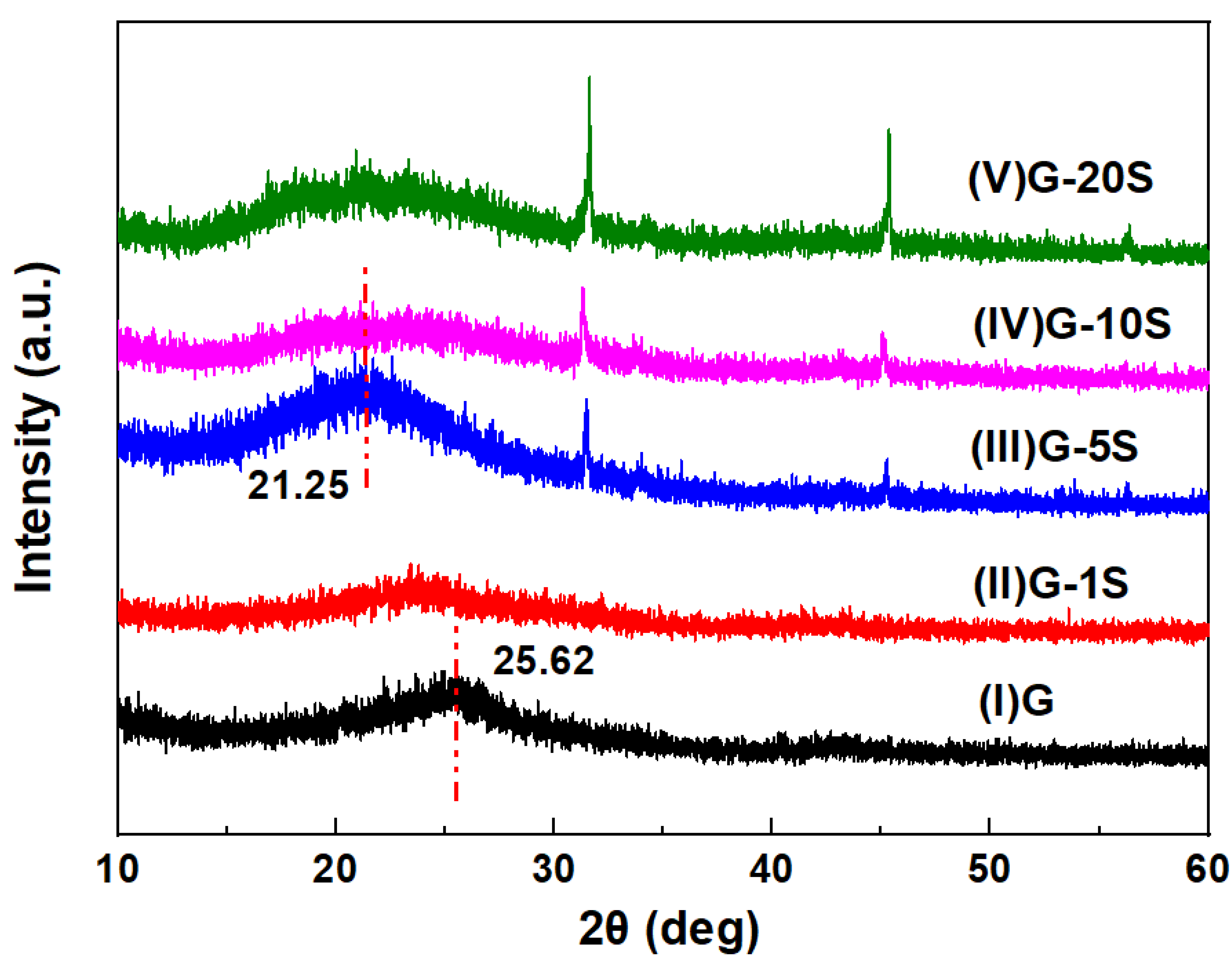
The crystallinity of the samples was subsequently examined to further understand the thickness and the quality of the graphene samples. Figure 6 shows specular 2θ XRD patterns of the graphene samples prepared with different SDBS proportions. It can be seen from Figure 6 that the (002) Bragg peak position of pure graphene (black curve) is at 2θ = 24.87°, while the (002) peaks of the modified graphene samples are at lower 2θ angles. The (002) peak of sample G-5S locates at 2θ = 20.85°, which is the lowest value. The Bragg equation, i.e., 2dsinθ = nλ (n = 1,2,3…) describes the relationship between the crystal plane spacing (d), the X-ray incident angle (θ), and the X-ray wavelength (λ). According to the Bragg equation, the interlayer spacing of each sample graphene can be calculated from the X-ray incident angle, and the results are shown in

Table 3. X-ray diffraction pattern of modified graphene sample (002) peak position and interlayer spacing.

Sample Number	G	G-1s	G-5s	G-10s	G-20s
(002) peak position (°)	24.87	23.45	20.85	20.91	20.91
Graphene layer spacing (nm)	0.358	0.379	0.426	0.424	0.424

. It can be seen from Table 3 that the graphene layer spacing of the unmodified sample G is the smallest, which is 0.358 nm, and sample G-5S has the largest graphene layer spacing, which is 0.426 nm.

Table 3 shows the corresponding relationship between the (002) peak position and the graphene layer spacing.

To elucidate the anti-corrosion performances of different epoxy samples, Tafel polarization examination was carried out. Figure 7 shows the Tafel polarization curves of E, EG0.1, ESG0.1, ES, EG0.5, and ESG0.5. The upper part of the curve is the anodic polarization curve, and the lower part is the cathodic polarization curve. By extending the straight part of the curves, one could find an intersected point of the extended lines, and the abscissa of the intersection is the value of the corrosion current. The corrosion rate of the metal can be estimated by evaluating the corrosion current density (the ratio of the self-corrosion current to the test area of the sample) I_corr, which represents the intensity of the cathodic oxygen reduction and anodic dissolution of metal ions [20]. When the logarithm of the corrosion current of the sample is less than −10 A, the logarithm of the I_corr of the sample is out of the detection range and thus the accurate value cannot be obtained. This indicates that the sample without immersion has strong anti-corrosion ability.

Table 4. Current density of E, EG0.1, ESG0.1, ES, EG0.5, and ESG0.5.

Number	E	ES	EG0.1	ESG0.1	EG0.5	ESG0.5
Current density log Icorr	−7.9	−8.5	<−10	<−10	−8.9	<−10

summarizes the corrosion current density of each sample in Figure 7. It can be concluded from Table 4 that the corrosion current densities of EG0.1, ESG0.1, and ESG0.5 are rather small, because the Tafel curves show only noise peaks, suggesting better anti-corrosion performance. On the contrary, the I_corr values of E and ES samples are larger and thus their anti-corrosion performances are worse.

Electrochemical impedance spectroscopy measurements were performed to study the impedance property of all the samples. Figure 8a–f shows the impedance spectroscopy of all samples after immersing in 3.5% NaCl solution for 0, 6, 12, 18, and 24 h, respectively. The impedance spectroscopy represents the relationship between the impedance modulus value and frequency. By analyzing the impedance modulus value of the sample at low frequencies, the anti-corrosion ability of the sample coating can be estimated [21,22].

For the sample E (Figure 8a), when it was not immersed, the impedance modulus value at 0.1 Hz is 1.25 × 10⁷ Ω. With the increase in immersion time, the impedance modulus value of sample E at 0.1 Hz decreased rapidly. When the immersion time was 12 h, the impedance modulus value decreased to 2.34 × 10⁴ Ω, and then as the immersion time increased, the impedance modulus value of 0.1 Hz was no longer significantly reduced. For the sample ES (Figure 8b), when it was not immersed, the impedance modulus value at 0.1 Hz is 5.88 × 10⁷ Ω, which is higher than the impedance modulus value of the sample E at 0.1 Hz when the sample E is not immersed. With the increase in the immersion time, the impedance modulus of the sample ES at 0.1 Hz decreased rapidly, but both were higher than the impedance modulus of the sample E under the same immersion time at 0.1 Hz. When the immersion time is 24 h, the impedance modulus of the sample ES at 0.1 Hz drops to 6.30 × 10⁴ Ω. For the sample EG0.1 (Figure 8c), when it was not immersed, the impedance modulus value at 0.1 Hz is 7.37 × 10⁸ Ω, which is higher than the impedance modulus value of the sample E, which indicates that the incorporation of graphene enhances the anti-corrosion ability of coating. As the immersion time increases, the impedance modulus value of the sample EG0.1 at 0.1 Hz decreases slowly. When the immersion time is 24 h, the impedance modulus value of the sample EG0.1 at 0.1 Hz is still close to 10⁷ Ω, which shows that the EG0.1 sample still has good corrosion resistance. For the sample EG0.5 (Figure 8d), when it was not immersed, the impedance modulus value at 0.1 Hz is 5.94 × 10⁷ Ω, which is higher than the impedance modulus value of the sample E at 0.1 Hz when not immersed, but lower than the sample EG0.1 at 0.1 Hz when not immersed. This shows that increasing the amount of graphene does not increase the corrosion resistance of the coating. This may be because the extra unmodified graphene cannot be stably dispersed in the epoxy coating, and the existence of graphene particles destroys the compactness of the epoxy coating. When the immersion time is 24 h, the impedance modulus value of the sample EG0.5 at 0.1 Hz is 2.47 × 10⁵ Ω, which is lower than the impedance modulus value of the sample EG0.1 at 0.1 Hz. The anti-corrosion ability of EG0.5 coating is weaker than that of EG0.1 coating. For the sample ESG0.1 (Figure 8e), when it is not immersed, the impedance modulus value at 0.1 Hz is 4.31 × 10⁹ Ω, which is the highest impedance modulus value of all samples at 0.1 Hz, indicating that the sample ESG0.1 has the strongest anti-corrosion ability of the coating. With the increase in immersion time, the impedance modulus of the sample ESG0.1 at 0.1 Hz decreases slowly. When the immersion time is 24 h, the impedance modulus of the sample ESG0.1 at 0.1 Hz is 1.92 × 10⁷ Ω, which is higher than that of the sample E. After the sample ESG0.1 is immersed for 24 h, the anti-corrosion ability of the coating is still higher than that of the sample E when it is not immersed. For the sample ESG0.5 (Figure 8f), when it was not immersed, the impedance modulus value at 0.1 Hz is 2.42 × 10⁹ Ω, which is second only to the ESG0.1 sample. With the increase in immersion time, the decreasing trend of the impedance modulus of the sample ESG0.5 at 0.1 Hz is basically the same as that of the sample ESG0.1 at 0.1 Hz. At the same immersion time, the impedance modulus of the sample ESG0.5 is lower than that of the sample ESG0.1 at 0.1 Hz. After being immersed for 24 h, the impedance modulus value of the sample ESG0.5 at 0.1 Hz is 1.15 × 10⁷ Ω, which is higher than of the sample E at 0.1 Hz without immersion, which means that the corrosion resistance of the coating after immersion for 24 h is still higher than that of the sample E without immersion.

Table 5. Impedance modulus of graphene-modified epoxy resin at 0.1 Hz frequency with different immersion times.

	Sample Number	E	ES	EG0.1	ESG0.1	EG0.5	ESG0.5
Immersion Time
0 h (Ω)		6.98	7.77	8.67	9.63	7.77	9.39
6 h (Ω)		5.07	7.39	8.03	9.42	7.36	9.09
12 h (Ω)		4.37	5.35	7.87	8.70	6.71	8.13
18 h (Ω)		4.39	5.23	7.64	7.85	6.23	7.44
24 h (Ω)		4.20	4.71	6.88	7.28	5.39	7.06

summarizes the impedance mode values of each sample at 0.1 Hz at different immersion times, and the corresponding image is shown in Figure 9. It can be seen from this figure that the impedance mode values of the sample ESG0.1 at low frequency are the highest at different immersion times among all samples, which means that the sample has the best corrosion resistance.

4. Conclusions

In conclusion, SDBS-modified graphene dispersion was successfully prepared by setting the mass ratio of SDBS to graphene as 1:1, 5:1, 10:1, and 20:1. The modified graphene can be stably dispersed in deionized water. AFM and Raman results showed that the 2D peak position of the modified graphene had a red shift, and when the mass ratio of SDBS to graphene was 5:1, the sample had the largest shift. AFM results showed that the thickness of graphene modified by SDBS was 4.71, 3.50, 4.12, and 4.15, respectively. At the same time, XRD results show that when the mass ratio of SDBS to graphene is 5:1, the interlayer spacing of modified graphene is the largest, which is 0.426 nm. Infrared results show the modified graphene powder contains SDBS, which indicates that the modification of graphene is formed by the interaction of SDBS and graphene. FIR results show that the chemical combination of sodium dodecylbenzene sulfonate and graphene occurs. The low-frequency impedance of samples decreases with the increase in the immersion time, and the impedance values from low to high are E, ES, EG, and ESG under the continuous immersion condition. The low-frequency impedance of the two ESG samples are the largest, which indicates that the corrosion resistance of these two samples is superior, and the corrosion resistance of ESG0.1 is even better than that of ESG0.5. Our results provide a guidance for controlling the interlayer spacing of graphene and improving the anti-corrosion performance of epoxy resin coatings, which is of great interest for anti-corrosive coating applications such as offshore facilities, transportation facilities, equipment in energy industry, petrochemical industry, etc.