Parametric Study of Ultrasonic De-Icing Method on a Plate with Coating

Abstract

Ultrasonic de-icing is a promising method to de-ice structures by using lightweight and simple transducers, with the advantage of low power consumption. A successful ultrasonic de-icing technique requires the understanding of the effects of different parameters on de-icing. This paper presents a thorough parametric study of the ultrasonic de-icing method on a plate with coating. First, the dispersion equations of shear horizontal (SH) and Lamb waves were derived based on the global matrix method. Meanwhile, interface shear concentration coefficients (ISCC) were introduced to represent the ability of ultrasonic de-icing, which was further integrated into Lamb wave and SH waves dispersion curves for the selection of optimal frequencies. Second, a three-layer plate model (host plate-coating-ice) was used to demonstrate the effect of different parameters of coating and the thickness of ice on ultrasonic de-icing. The theoretical model provided the design principle of coating and ultrasonic parameters required for efficient de-icing. Finally, an experiment was conducted on an ultrasonic de-icing platform to validate the proposed ultrasonic de-icing method. In this process, material parameters including the Young’s modulus, thickness of coating, and thickness of the ice layer were analyzed. The trends of power consumption and optimal frequency of experiments are in good agreement with the analytical calculated results.

1. Introduction

For structures in cold environments, freezing is a critical issue, that must be solved in order to guarantee the workability of structures. The accumulation of ice on structures would detrimentally affect performance and reliability. Ice accretions have serious impacts on performance of offshore platforms, marine vessels [1,2,3,4], aircraft [5,6], wind turbine blades [7,8], power line [9] etc. Over the past decades, several thermal and mechanical methods associated with de-icing have been developed, including pneumatic, electro-thermal, electro-impulse, vibratory, etc. [6,10,11]. However, these technologies are limited due to energy and weight constraints [12]. Take the widely used thermal de-icing methods for aircraft as an example, the electrothermal de-icing system is heavily up to 162 lbs. and requires power 25 kW. Therefore, the electrothermal de-icing system can only operate for short periods. After the deicing system is turned off, the liquid on the aircraft can freeze again [13]. An ultrasonic de-icing system [5,14,15] is promising for achieving de-icing by using lightweight and simple transducers, thus having the advantage of low power consumption.

Several studies regarding de-icing have been conducted by using ultrasonic guided waves (UGW). Ramanathan et al. [16] developed and validated the possibility and feasibility of using shear horizontal waves to detach the ice layer from an iced aluminum plate. In their experiment, shear horizontal waves were generated to deice the aluminum plate by melting the ice at the interface. However, instantaneous ice delamination was not observed in the experiment. Palacios et al. [17] used piezoelectric actuators with resonance frequencies to de-bond the ice layer from an aluminum plate. The system was able to detach 1–3 mm thin ice layer from an aluminum plate at the resonance frequencies. To provide deicing for the entire structure of the blades, a dual de-icing system combining ultrasonic guided waves and low frequency vibration for wind turbine blades was explored by Habibi et al. [18]. In their study, only 2400 W was required for a 75 kW wind turbine de-icing, which is only 3.2% of the turbine’s nominal power output. An optimizing structural design method was used by introducing tailored waveguides (TWG) to enhance the shear stress at the interface between the host structure and the ice layer was analyzed by Zhu et al. [19]. MK Kalkowski et al. [20,21] proposed an approach to model piezoelectric excitation and remove unwanted accretions through a semi-analytical finite element (SAFE) method. This technique could model different types of actuators without the need for common simplifications regarding their dynamic behavior. Based on these, the shear stress and power required for deicing were investigated. Wang et al. [22] proposed a method to assess and predict the ultrasonic de-icing efficiency for composite wind turbine blades. In the study, the interface integrity extent (IIE) and its rate of change were defined and verified to describe the behavior of ice de-bonding. Daniliuk et al. [23] compared the performance of semi-hard lead zirconate titanate (PZT-4), lead magnesium niobate-lead titanate (PMN-PT) and lithium niobate (LiNbO₃) materials by ultrasonic transducers on de-icing for both aluminum and composite plates. However, previous studies have few reports regarding parametric studies for the host plate-coating-ice layered structure.

Corrosion of coating and anti-icing coatings [24,25] are widely used on structures, and affect the ultrasonic propagation in the process of de-icing. Therefore, it is necessary to study the effects of the coating parameters on ultrasonic de-icing to provide guidance for parameter designs of the host plate-coating-ice-layered model and achieve de-icing with less power. In this study, based on the theory of ultrasonic guided wave propagation in a multi-layer plate, the interface shear stress coefficient concentration (ISCC) [15], between the coating and ice layer for both Lamb and shear horizontal waves, were derived. To select the optimal exciting frequency, which has the maximum de-icing efficiency, ISCC was further integrated into dispersion curves, which were then computed via the global matrix method (GMM) [26,27] and the SAFE method for mutual validation in this study. The effect of material parameters on ultrasonic de-icing was predicted and discussed, including the coating’s Young’s modulus, thickness, density, Poisson’s ratio, and ice layer thickness. In addition, an ultrasonic de-icing experimental platform was built, and de-icing experiments were conducted to verify the effects of different parameters on de-icing.

2. ISCC value and Demonstration

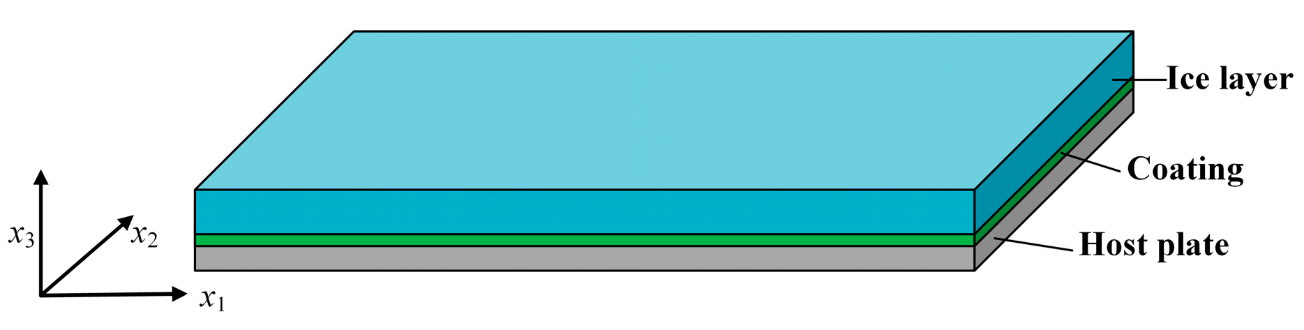
2.1. Dispersion Equations of a Plate with Coating and Ice Layers

A schematic of a general three-layer plate is illustrated in Figure 1. This plate consists of a host plate, coating, and ice layer. Interfacial shear stress between the ice layer and coating will be focused on for studying de-icing.

Lamb waves and shear horizontal (SH) waves are the two main types of ultrasonic guided waves, which contribute to interfacial shear stress. The governing equation for waves propagating in a single layer plate can be presented as follows,

$$\rho \frac{{\partial }^2{u}_i}{\partial t^2}=C_{ijkl}\frac{{\partial }^2{u}_i}{\partial x_j\partial x_k} (i=1,2,3)$$

(1)

where C_ijkl, ρ, and u_i are the stiffness matrix tensor, density, and the displacement field, respectively [27]. In Equation (1), u_i can be assumed as having the following solution,

$$u_i=U_i{\mathrm{e}}^{ik(x_1+\alpha x_3-ct)} (i=1,2,3)$$

(2)

where U_i is the polarization vector, k is the wave number along the x₁ direction, c represents the phase velocity along the x₁ direction, and α is the ratio of the wave number in the x₃ direction with respect to the wave number in the x₁ direction. The guided waves are assumed to propagate along the x₁ direction. The displacements for the Lamb waves exist in the x₁ and x₃ directions, while the displacement for SH wave exists only in the x₂ direction. By substituting Equation (2) into Equation (1), the following Christoffel Equation is obtained [27],

$$\left[\begin{array}{ccc}{\lambda }_{11}-\rho c^2& {\lambda }_{12}& {\lambda }_{13}\\ {\lambda }_{12}& {\lambda }_{22}-\rho c^2& {\lambda }_{23}\\ {\lambda }_{13}& {\lambda }_{23}& {\lambda }_{33}-\rho c^2\end{array}\right]\left\{\begin{array}{c}{U}_1\\ U_2\\ U_3\end{array}\right\}=\left\{\begin{array}{c}0\\ 0\\ 0\end{array}\right\}$$

(3)

$${\lambda }_{im}=C_{iklm}{n}_k{n}_l (i,j,k,l,m=1,2,3)$$

(4)

where n_k and n_l are the directional cosines of the normal to the wave front. The solutions of the Christoffel Equation (3) are referred to as partial wave solutions, for which linear combinations consist of the displacement and stress fields for Lamb and SH waves. In the case of Lamb waves, u₂ is equal to zero. The displacements and stresses can be expressed as Equations (5)–(8) with undetermined coefficients B_k, wherein B_k is the weighting coefficient of the partial waves. U_3k is the ratio of the polarization vectors between U₃ and U₁, which are obtained by solving the Christoffel Equation (3):

$$u_1={\displaystyle \sum _{k=1}^4{B}_k{\mathrm{e}}^{ik(x_1+{\alpha }_k{x}_3-ct)}}$$

(5)

$$u_3={\displaystyle \sum _{k=1}^4{B}_k{U}_{3k}{e}^{ik(x_1+{\alpha }_k{x}_3-ct)}}$$

(6)

$${\sigma }_{31}={\displaystyle \sum _{k=1}^4{B}_k\left[{\alpha }_k+U_{3k}\right]\mu \left(ik\right){\mathrm{e}}^{ik(x_1+{\alpha }_k{x}_3-ct)}}$$

(7)

$${\sigma }_{33}={\displaystyle \sum _{k=1}^4{B}_k\left[\lambda +\left(\lambda +2\mu \right){\alpha }_k{U}_{3k}\right]\left(ik\right){\mathrm{e}}^{ik(x_1+{\alpha }_k{x}_3-ct)}}$$

(8)

here, λ and μ are Lamé constants. For SH waves, only the displacement u₂ and stress σ₃₂ exist. Therefore, they can be expressed as follows:

$$u_2={\displaystyle \sum _{k=1}^2{B}_k{\mathrm{e}}^{ik(x_1+{\alpha }_k{x}_3-ct)}}$$

(9)

$${\sigma }_{32}={\displaystyle \sum _{k=1}^2{B}_k{\alpha }_k\mu \left(ik\right){\mathrm{e}}^{ik(x_1+{\alpha }_k{x}_3-ct)}}$$

(10)

In order to obtain the solutions of the undetermined coefficients B_k, traction free boundary conditions at the bottom and top surfaces of the plate are considered:

$${\sigma }_{3i}|{}_{\mathrm{bottom} \mathrm{surface}}=0 (i=1,2,3)$$

(11)

$${\sigma }_{3i}|{}_{\mathrm{top} \mathrm{surface}}=0 (i=1,2,3)$$

(12)

For a multi-layered plate, the stress and displacement continuity at the interfaces between adjacent layers are necessary and presented as follows,

$$u_i|{}_{\mathrm{top}}^k=u_i|{}_{\mathrm{bottom}}^{k+1} (i=1,2,3)$$

(13)

$${\sigma }_{3i}|{}_{\mathrm{top}}^k={\sigma }_{3i}|{}_{\mathrm{bottom}}^{k+1} (i=1,2,3)$$

(14)

where the superscript “k” represents the k-th layer, and the subscripts “top” and “bottom” represent the locations of interfaces between layers. Combining the boundary conditions of Equations (11) and (12), and the interfacial continuity of Equations (13) and (14), one linear homogenous equation set can be obtained as indicated in Equation (15), which follows the basic formalization of the global matrix method (GMM). The detailed derivation process of the GMM is presented in Ref. [27], and thus, will not be presented here for brevity.

$${\mathit{D}}_N\mathit{B}=0$$

(15)

In Equation (15), D_N is the global matrix that connects frequency f and phase velocity c. The subscript “N” represents the number of layers in a multi-layered plate. B is the vector of the undetermined weighting coefficients of all layers. Equation (15) should have non-trivial solutions of B, which requires the vanished D_N, that is, its determinant should be zero. The dispersion curves of Lamb and SH waves can be obtained by solving $\left|{\mathit{D}}_N(f,c)\right|=0$ via numerical methods. In this study, the bisection method was used because of its simplicity. Then, for a certain point (f,c) in the dispersion curves, substituting it into Equation (15), one can obtain the non-trivial solutions of B. Finally, substituting the weighting coefficients B_k of each layer into Equations (5) through (10) can obtain the wave structure of displacements and stresses corresponding to the point (f,c) in the dispersion curves.

In each isotropic layer, there are four partial waves for Lamb waves and two for SH waves based on the partial wave theory [18]. Therefore, the matrix order of D_N in Equation (15) should be 4N × 4N for Lamb waves and 2N × 2N for SH waves. The vector dimension of B follows the same rule to be compatible with D_N.

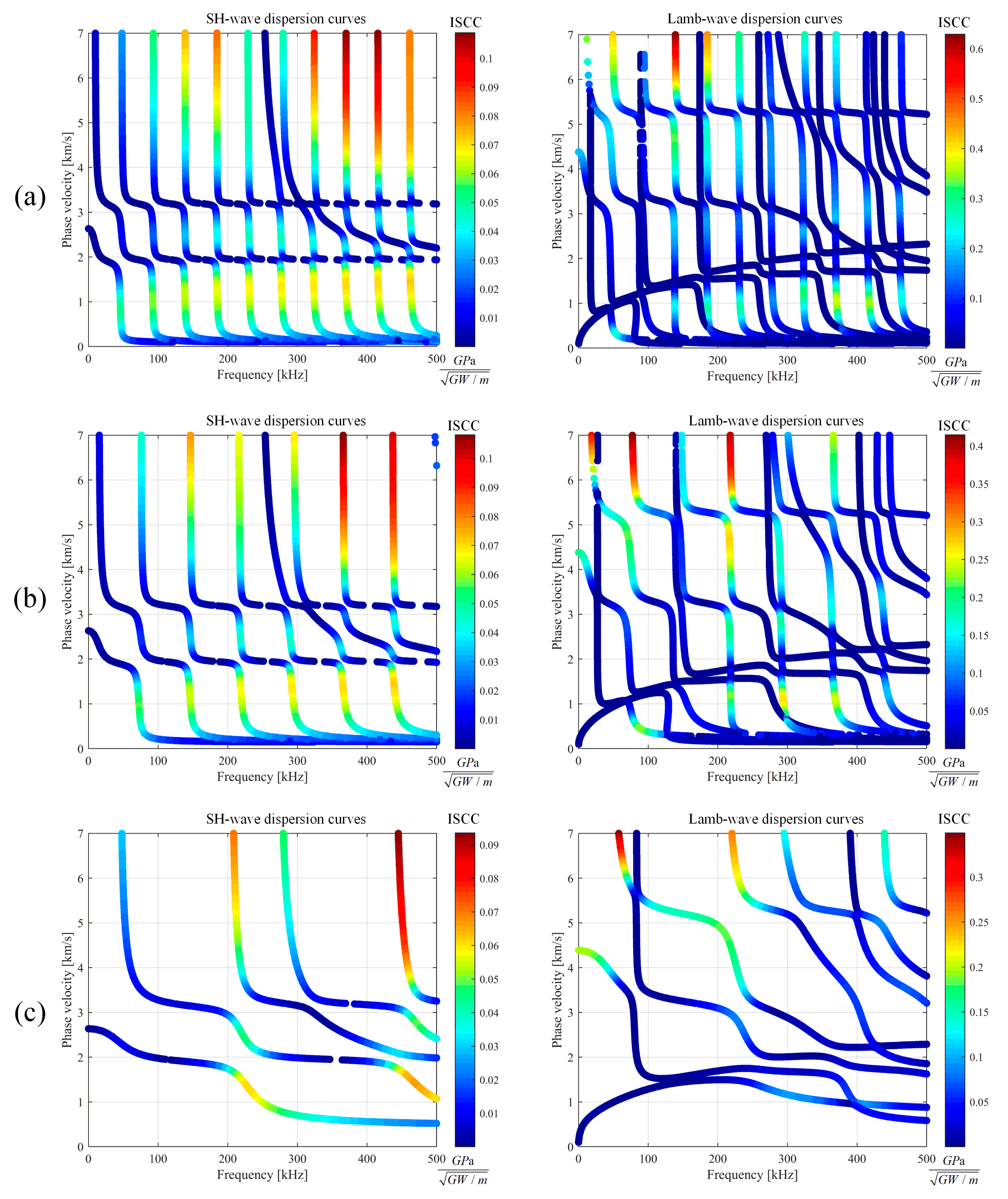
2.2. ISCC Values of SH and Lamb Waves

To estimate the ability of inducing stress at the interface from a given amount of power, the concept of interfacial stress concentration coefficients (ISCC) is proposed to calculate the normalized interface shear stress for different ultrasonic guided wave modes and frequencies [15]. The larger the ISCC, the larger the modal shear stress at interface will be induced for a given power, and vice versa [28]. The complex acoustic Poynting’s vector is defined as the power flow on the structure, expressed as Equation (16), where v is the particle velocity defined in Equation (17); “*” represents the complex conjugate; σ is the stress tensor:

$$\mathit{P}=-\frac{{\mathit{v}}^{*}·\mathit{\sigma }}{2}$$

(16)

$$\mathit{v}=\left[\begin{array}{ccc}\frac{\partial u_1}{\partial t}& \frac{\partial u_2}{\partial t}& \frac{\partial u_3}{\partial t}\end{array}\right]$$

(17)

The total power flow can be obtained by integrating the x₁ component $p_{x_1}$ in P across the entire thickness of a multi-layered plate and is expressed as follows:

$$Power={\displaystyle {\int }_{\mathrm{Thickness}}{p}_{x_1}}d{x}_3$$

(18)

The ISCC values for SH and Lamb waves are defined in Equations (19) and (20), respectively, [28],

$$ISC{C}_S=\frac{{{\sigma }_{32}|}_{\mathrm{Layer} \mathrm{interface}}}{\sqrt{power}}$$

(19)

$$ISC{C}_L=\frac{{{\sigma }_{31}|}_{\mathrm{Layer} \mathrm{interface}}}{\sqrt{power}}$$

(20)

where, the subscripts “S” and “L” indicate SH, and Lamb waves, respectively.

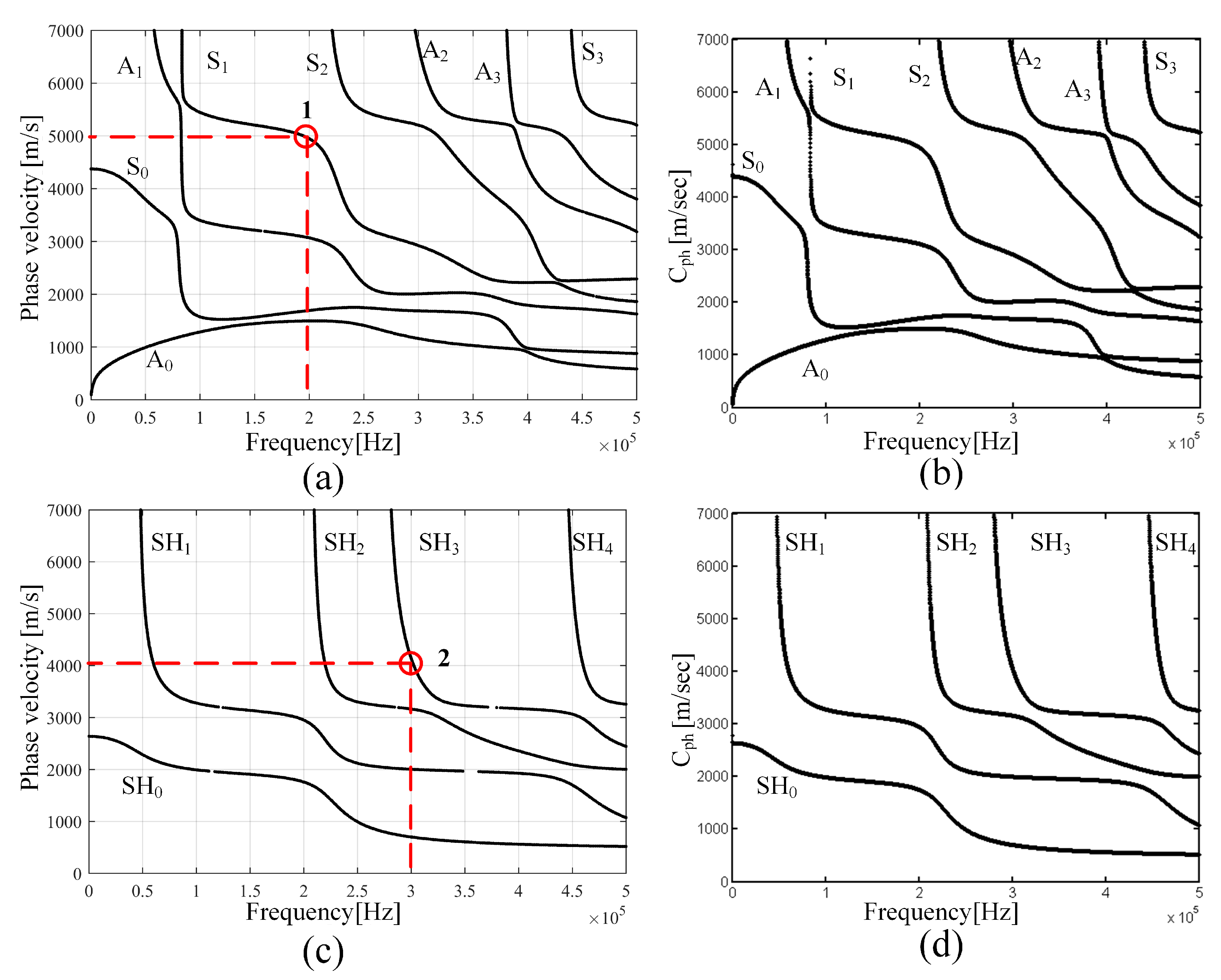
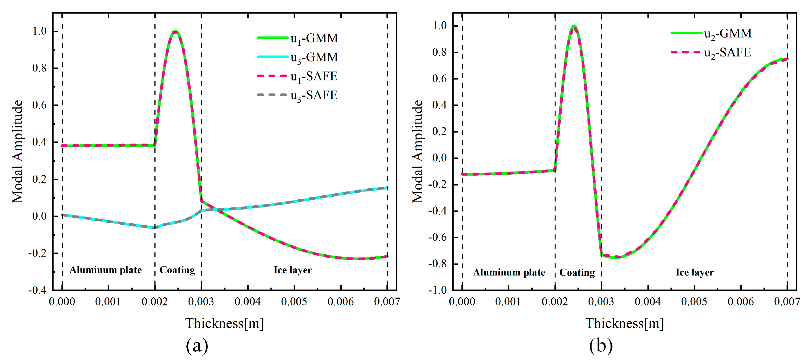
2.3. Demonstration of Computing Dispersion Curves and Wave Structures on a Three-Layered Plate Model

To demonstrate the accuracy of the computing dispersion curves and wave structures by using GMM, which is a prerequisite for studying ultrasonic de-icing, a three-layered plate model (host plate-coating-ice layer) was used. The material properties of the three layers are listed in

Table 1. Material Properties.

Layer	Density (kg/m3)	Young’s Modulus (GPa)	Poisson’s Ratio	Thickness (mm)
Ice	920	9.1	0.28	4
Coating	900	0.5	0.30	1
Aluminum	2700	70	0.27	2

.

Given that there are three layers, N = 3 in Equation (15). By using GMM, the computed dispersion curves of the three-layered structure for both Lamb and SH waves are shown in Figure 2a,c, respectively. In Figure 2b,d, the same type of dispersion curves computed via the software GUIGUW [29], which is based on the SAFE method, are provided for comparison. Apparently, both methods present sufficient agreement, which demonstrates the accuracy of GMM used in this study. Meanwhile, it can be found that there are 8 modes for Lamb waves and 5 modes for SH waves in the frequency range considered.

In addition, the wave structures obtained using GMM were compared with those of SAFE method. Figure 3a,b present the typical displacement wave structures over the plate thickness for S₁ and SH₃ modes, which correspond to points 1 and 2 in Figure 2, respectively. As shown in Figure 3, sufficient agreements between the two methods are also obtained, which further demonstrates the reliability of GMM.

It should be noted that GUIGUW cannot compute the stress wave structure and power flow with the current version, which is required for calculating ISCC. Therefore, in the following sections, all computations are only involved in GMM owing to its comprehensiveness.

3. Results and Discussion

3.1. Parametric Study on ISCC

Considering that the ISCC value of a certain mode at a certain frequency represents the ability of ultrasonic de-icing, in this section, a parametric study of the coating properties and ice layer thickness on ISCC is presented. For the convenience of comparing different ISCC values, one can superimpose them on dispersion curves, as illustrated in Figure 4. The three-layered plate model used in this section is still based on Section 2.3, and the layers’ basic material properties are provided in Table 1. When studying a certain factor, the values of all other factors are fixed according to the controlling variate method.

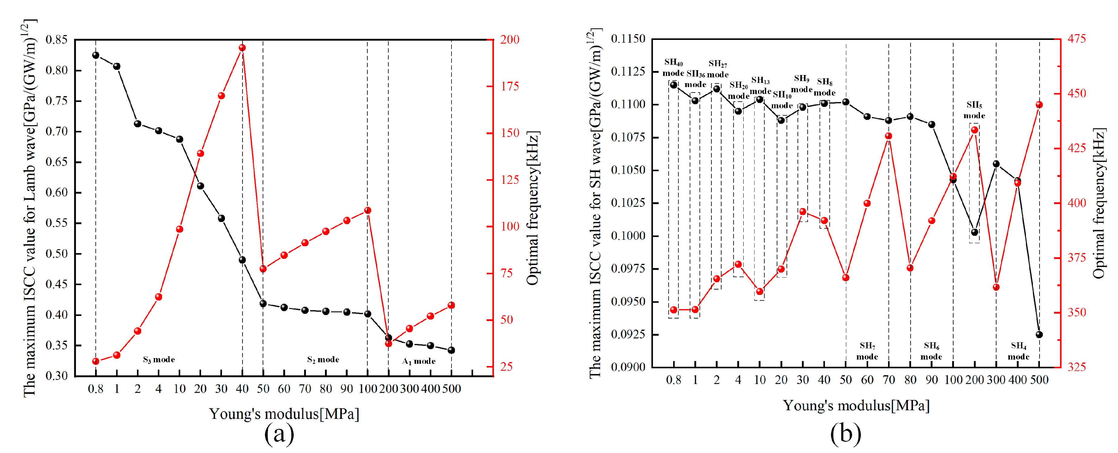
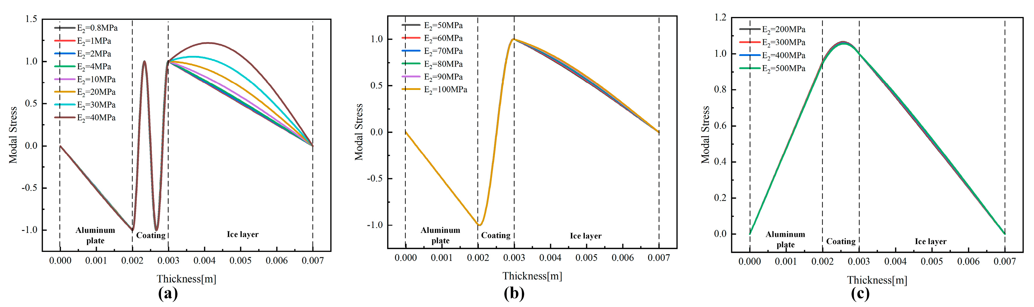
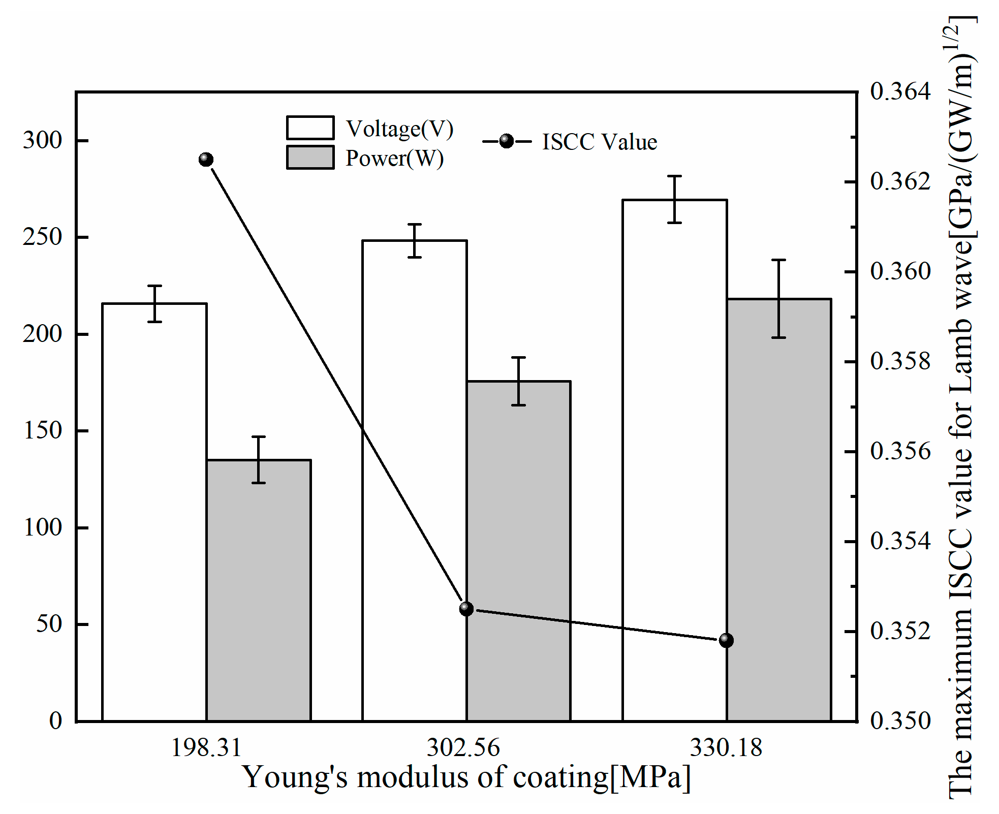
3.1.1. Effect of Young’s Modulus of the Coating

For this factor, the density of the ice layer was 917 kg/m³ and the Poisson’s ratio was 0.31. The other material parameters were the same as those mentioned in Table 1, except for the Young’s modulus of the coating, which varied from 0.8 MPa to 500 MPa to form 18 Young’s moduli and are marked in the x-axis of Figure 5 to be the detailed reference. The maximum phase velocity and frequency were considered to be 7 km/s and 500 kHz, respectively.

An example of ISCC values superimposing on dispersion curves (SH and Lamb waves) corresponding to three different Young’s moduli of the coating are shown in Figure 4. With the increasing of Young’s modulus, fewer modes of both SH and Lamb waves appear in the considered frequency range. Especially for Lamb waves, the number of modes increases dramatically with the decrease in Young’s modulus. The maximum ISCC value for Lamb waves decreases with the increasing of Young’s modulus, but that for SH waves without a regular pattern. In addition, the optimal mode corresponding to the maximum ISCC would change from a low-order mode to high-order mode with the decrease in the Young’s modulus of coating. Finally, in the considered frequency range and at the same Young’s modulus, the maximum ISCC appeared in Lamb waves is bigger than the one in SH waves, which indicates Lamb waves producing a higher de-icing efficiency than SH waves.

The maximum ISCC values for Lamb and SH waves corresponding to the 18 Young’s moduli of coating are summarized in Figure 5. For Lamb waves in Figure 5a, the maximum ISCC values decrease with an increase in Young’s modulus. When the Young’s modulus is within 0.8 MPa and 40 MPa, the maximum ISCC always appears in the S₃ mode. However, for the other two ranges of Young’s modulus, it appears in the S₂ and A₁ modes. Figure 5a also presents the optimal frequency (see the right y-axis) corresponding to the maximum ISCC for each Young’s modulus. When Young’s modulus lies within each separated range (range 1 from 0.8 MPa to 40 MPa, range 2 from 50 MPa to 100 MPa, range 3 from 200 MPa to 500 MPa), the optimal frequency increases with the increase in Young’s modulus. For SH waves in Figure 5b, the maximum ISCC values decrease with an increasing Young’s modulus in a whole, which correspond to 12 different modes. However, the changing tendency of the optimal frequency at the maximum ISCC value is irregular with the increasing of Young’s modulus. In the same mode, the optimal frequency increases with an increase in the Young’s modulus of the coating. Comparing both figures, the changing range of the maximum ISCC value for Lamb waves (0.30–0.85) is significantly greater than that of the SH waves (0.090–0.115) when the Young’s modulus varies from 0.8 MPa to 500 MPa. The optimal frequencies in Lamb waves usually appear in the lower frequency range (20 kHz–200 kHz), but a relatively higher frequency range (325 kHz–475 kHz) is focused for SH waves. Therefore, the shear stress σ₃₁ wave structures of Lamb waves corresponding to the maximum ISCC for these 18 groups were further analyzed.

These wave structures were normalized such that the value at the interface between the coating and ice layer was equal to 1 to enable comparison of wave structure trends. The results are shown in Figure 6. For different ranges of the Young’s modulus, the wave structure of σ₃₁ presents different forms because they belong to different modes while at different frequencies. Considering that the wave structure of σ₃₁ at a Young’s modulus of 200 MPa is the smoothest (see Figure 6c), which are most suitable for coating applications in engineering, the Young’s modulus of the coating was fixed at 200 MPa in the following study.

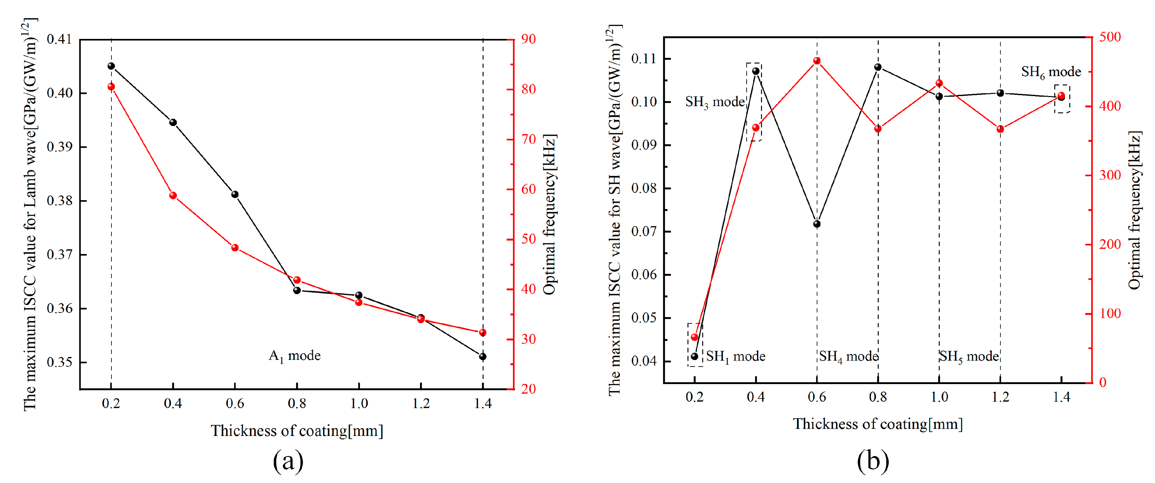
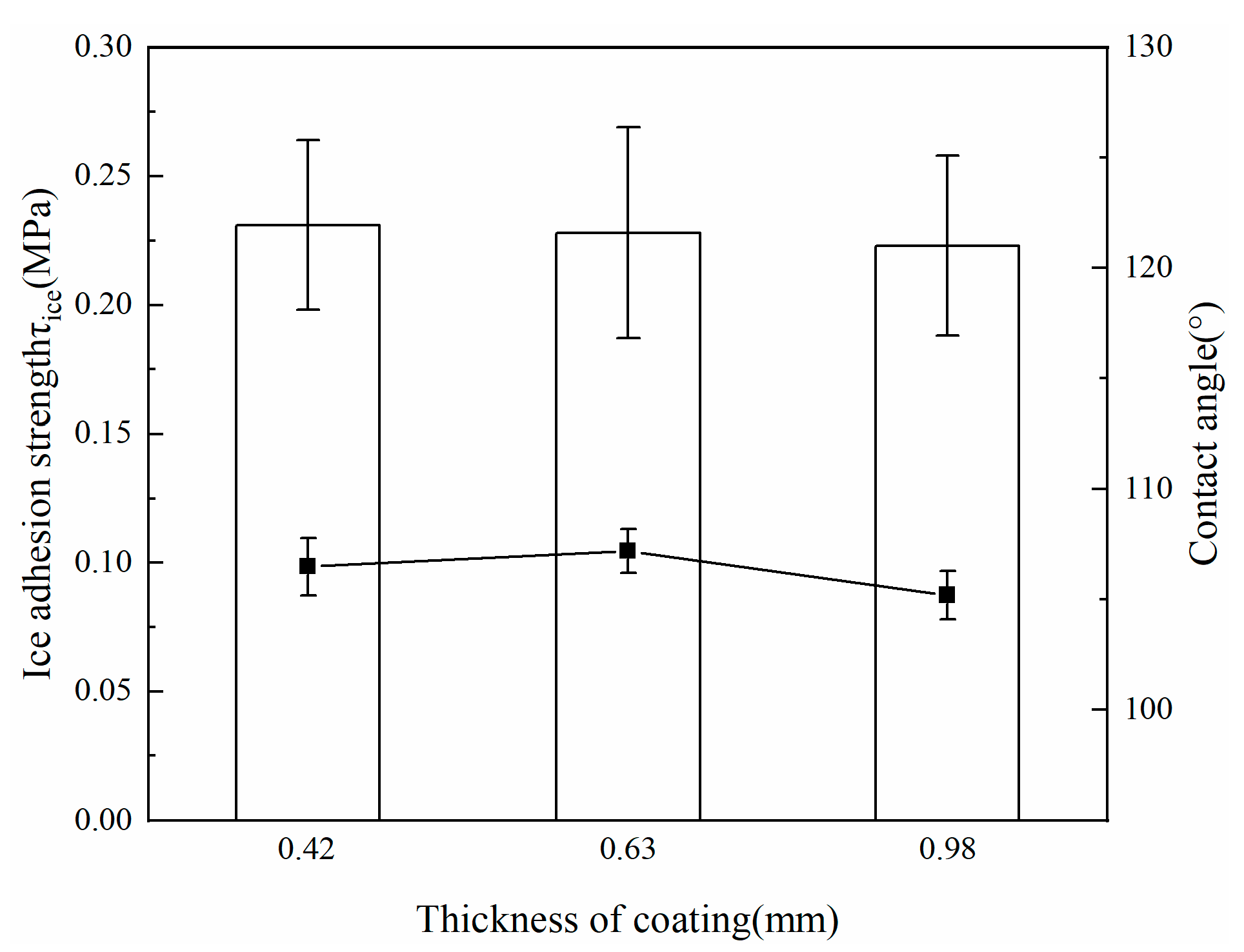
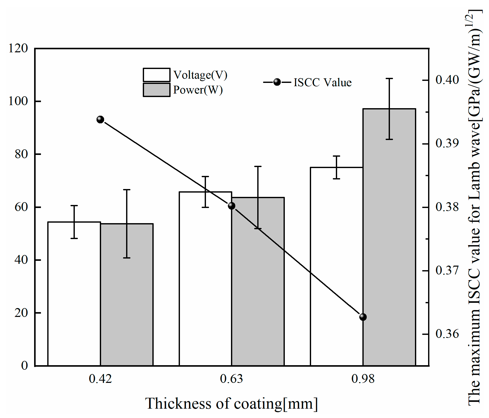
3.1.2. The Effect of Coating Thickness

The Young’s modulus of the coating was assigned as 200 MPa based on the results of Section 3.1.1. The other material parameters were the same as those described in Section 3.1.1. The thickness of the aluminum plate and ice layer were 2 mm and 4 mm, respectively, while the coating thickness varied from 0.2 mm to 1.4 mm. The effects of coating thickness on the maximum ISCC values and optimal frequency were calculated and shown in Figure 7.

As shown in in Figure 7a, both the maximum ISCC values and optimal frequencies for Lamb waves decrease with the increasing of the coating thickness. Meanwhile, the maximum ISCC values always appear in A₁ mode of Lamb waves. For the SH waves, shown in Figure 7b, when the coating thickness varies from 0.4 mm to 1.4 mm, the maximum ISCC values change around 0.1 $\mathrm{GPa}/\sqrt{\mathrm{GW}/\mathrm{m}}$ and the optimal frequencies change around 400 kHz. When the coating thickness is 0.2 mm, both the optimal ISCC and the optimal thickness stay in their respective minimum level (for ISCC 0.04 $\mathrm{GPa}/\sqrt{\mathrm{GW}/\mathrm{m}}$ and for optimal frequency 66.37 kHz). Unlike Lamb waves, the maximum ISCC in SH waves appear in five different modes, as indicated in Figure 7b, with the increasing of coating thickness. Significantly, the ISCC values for the SH waves are relatively small compared to the Lamb waves (see Figure 7). Therefore, the concern to the influence of Lamb waves on de-icing should be more focused on than SH waves at the same coating thickness. Meanwhile, if coatings with different thicknesses correspond to the same optimal de-icing mode in the dispersion curves, properly reducing the thickness of the coating may improve the de-icing efficiency.

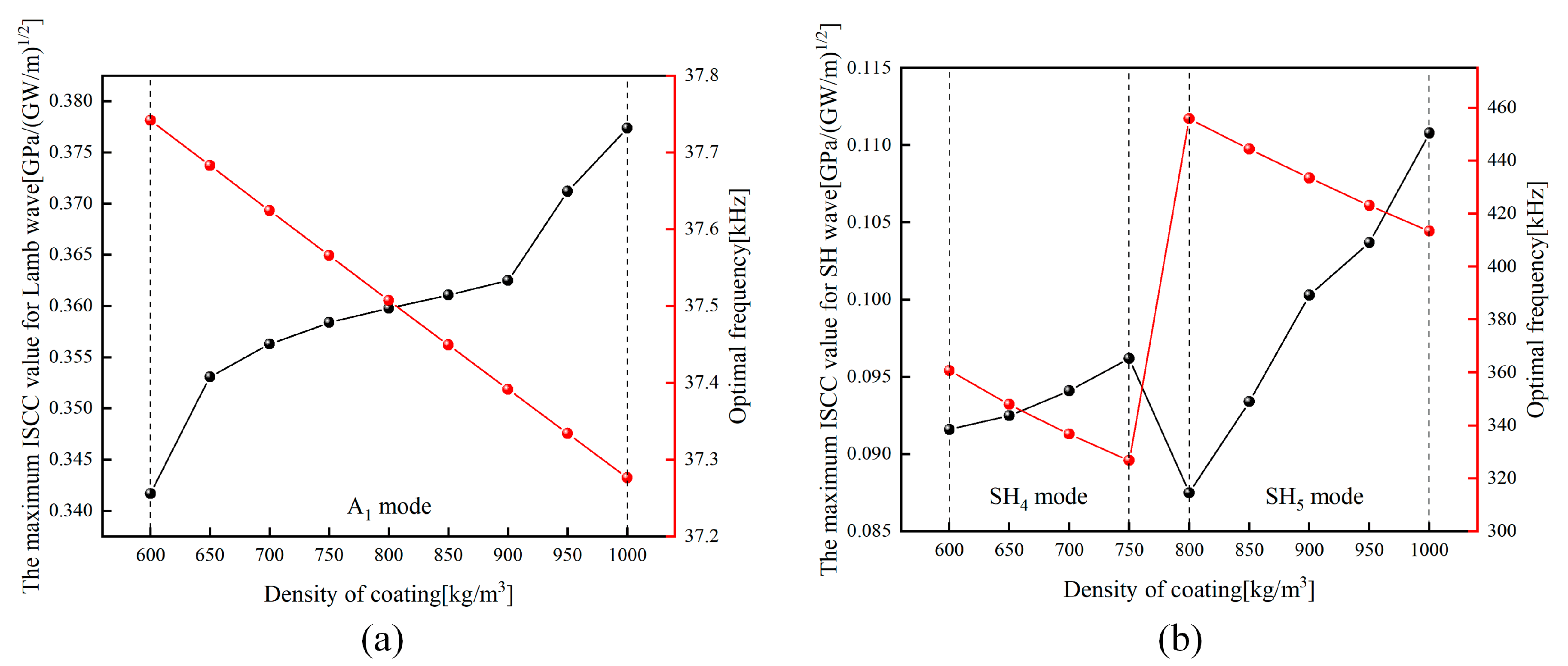
3.1.3. The Effect of Coating Density

Based on the results above, the Young’s modulus and thickness of coating were 200 MPa and 1 mm, respectively. The other parameters were the same as those mentioned prior. The coating density varied from 600 kg/m³ to 1000 kg/m³. The thickness of the aluminum plate and ice layer were 2 mm, and 4 mm, respectively. As shown in Figure 8, when the coating density increases from 600 kg/m³ to 1000 kg/m³, the maximum ISCC values for Lamb waves slightly increase as well, and they appear in the A₁ mode. As for the optimal frequency of Lamb waves, it linearly decreases with the increasing of coating density whereas slightly changing (from 37.8 kHz to 37.2 kHz). Turn to the case of SH waves shown in Figure 8b, two separated ranges of coating density can be observed (range 1 from 600 kg/m³ to 750 kg/m³ and range 2 from 800 kg/m³ to 1000 kg/m³). In each range, the maximum ISCC values slightly increase with the increase in coating density, meanwhile they appeared in the same mode (SH₄ mode for range 1 and SH₅ mode for range 2). Similarly, the optimal frequencies notably decreased with the increasing of coating density at each range. Comparing both figures, it can be concluded that the coating density has little impact on the de-icing effect (ISCC value); however, it significantly affects the optimal frequency in SH waves. Therefore, the expected de-icing frequency range can be obtained by adjusting the coating density and optimally adjusting the coating density can achieve the maximum efficiency of de-icing.

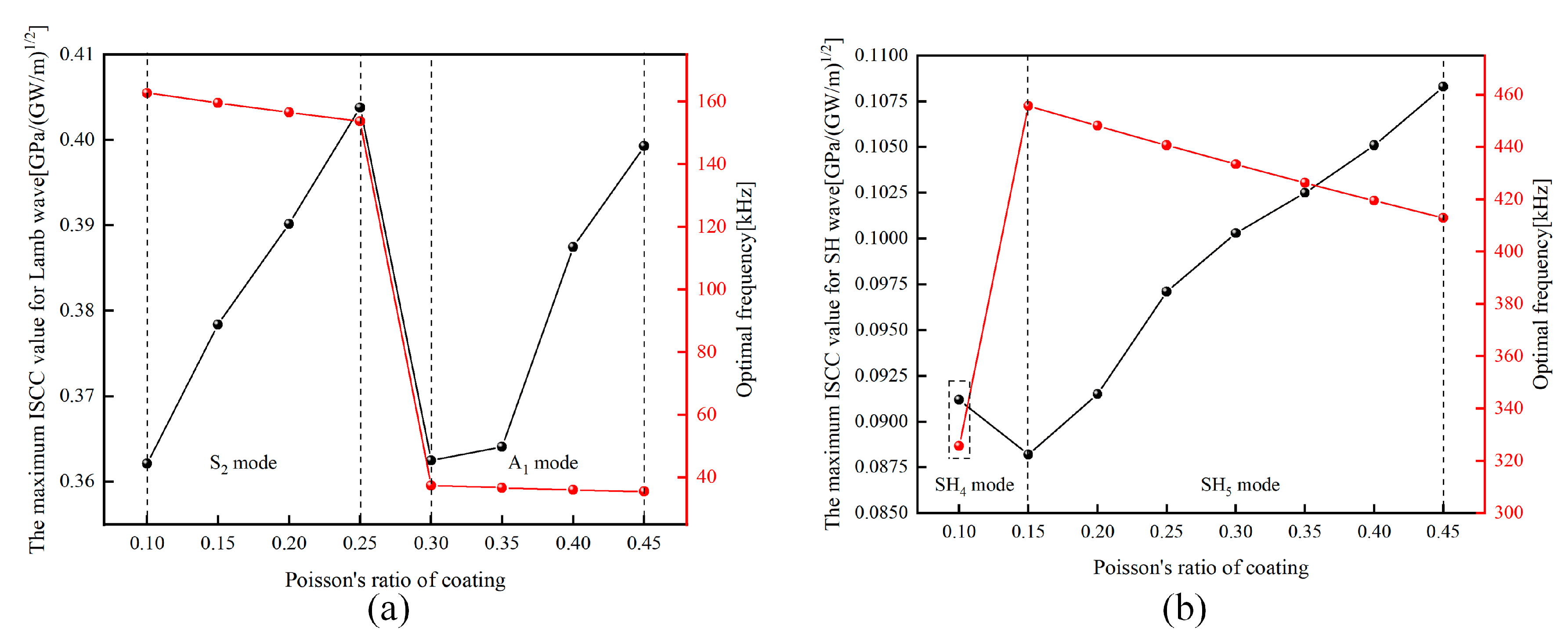
3.1.4. The Effect of Coating Poisson’s Ratio

In this section, the coating Young’s modulus was 200 MPa, the density was assigned to be 900 kg/m³, and the Poisson’s ratio varied from 0.10 to 0.45. Similar processes were performed, and the results are shown in Figure 9.

For Lamb waves, there are two ranges of Poisson’s ratio that affect the maximum ISCC value and the optimal frequency, range 1 from 0.1 to 0.25 and range 2 from 0.30 to 0.45. The maximum ISCC appears in S₂ and A₁ mode when Poisson’s ratio varies in range 1, and 2, respectively. It can be also seen from Figure 9a that in each range, the maximum ISCC increases and the optimal frequency decreases with the increasing of Poisson’s ratio. For SH waves, shown in Figure 9b, except for the least Poisson’s ratio 0.10, the maximum ISCC increases and the optimal frequency decreases with the increasing of Poisson’s ratio, meanwhile they appear all in SH₅ mode. Based on the results above, it can be concluded that appropriately increasing the Poisson’s ratio is beneficial to de-icing.

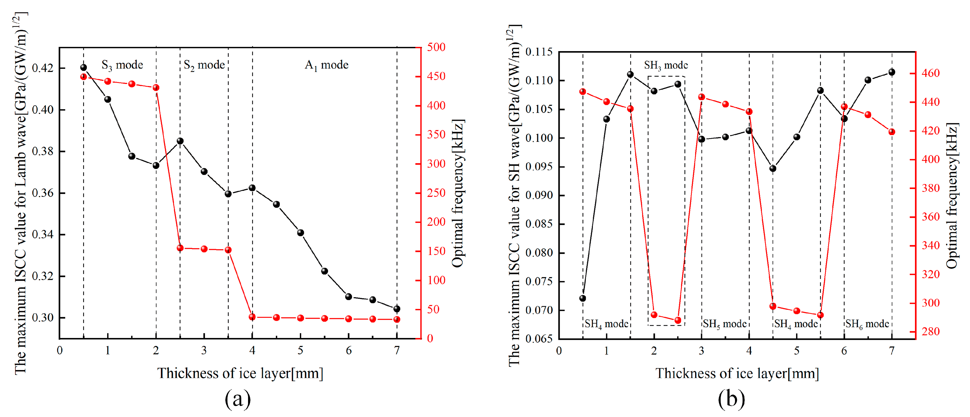
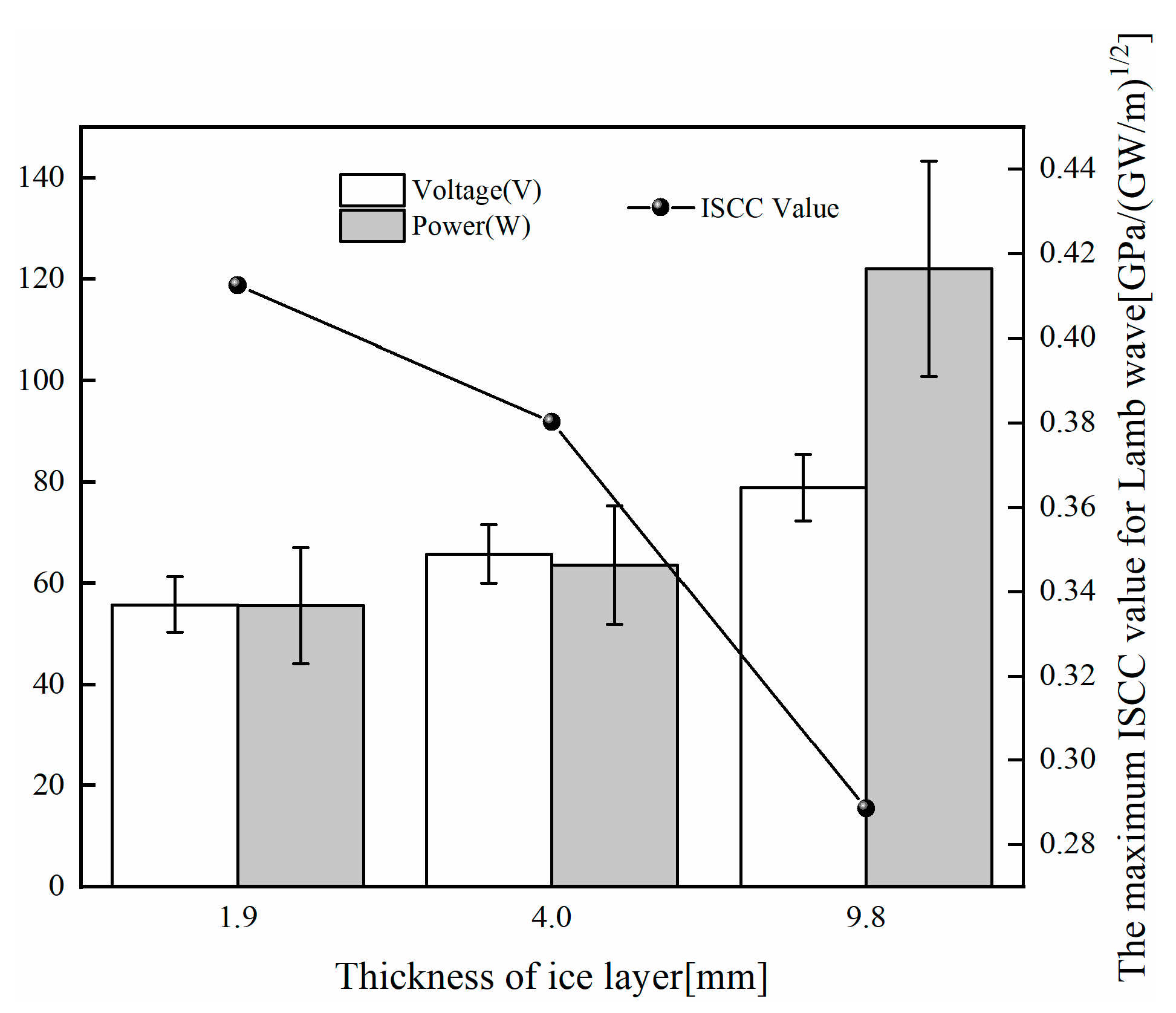
3.1.5. The Effect of Ice Thickness

In this section, the focus is switched to the property of ice, studying the effect of ice thickness on the maximum ISCC value. The Young’s modulus of the coating was 200 MPa; the density was 900 kg/m³; the Poisson’s ratio was 0.30; and the thickness was 1 mm. The thickness of the ice layer varied from 0.5 mm to 7 mm. Figure 10 shows the computed results. For Lamb waves, the maximum ISCC values appear in three modes (S₃, S₂, and A₁) when the thickness of ice layer varies in three ranges as shown in Figure 10a. Synchronously, the maximum ISCC and the optimal frequency decrease with the increasing of the thickness of ice layer in each range. For SH waves, shown in Figure 10b, the effects of the thickness of ice layer on the maximum ISCC and optimal frequency are complex, because the thickness of ice layer is separated into five ranges. At the boundary of any two adjacent ranges, the maximum ISCC and the optimal frequency change suddenly. When different thicknesses of the ice layer correspond to the same optimal mode, the ISCC value increases and the optimal frequency decreases with the increase in ice thickness. Comparing both figures, the ISCC values of SH waves are significantly smaller than those of Lamb waves. Thus, adopting Lamb waves to de-icing is more efficient than SH waves. The ISCC values for both Lamb waves and SH waves present a non-monotonic behavior. This finding indicates that it is possible to reduce de-icing energy consumption by reasonable selecting the de-icing thickness of the structure.

Based on the analysis of the five parametric studies above, a few conclusions can be reached. The maximum ISCC values for Lamb waves are greater than those of SH waves at the same material properties. Compared to adopting Lamb waves, using SH waves to de-icing is more sensitive to changes of material properties, which adds a lot of difficulties for designing an optimal de-icing system. In a word, employing Lamb waves to de-icing is preferred, meanwhile the lower frequency range should be focused on.

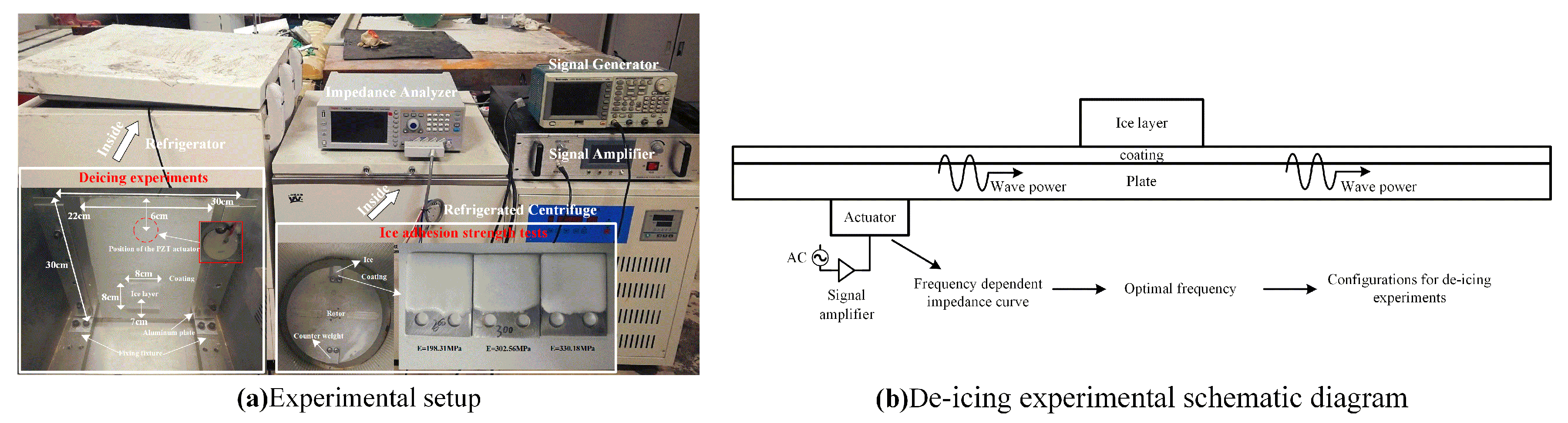
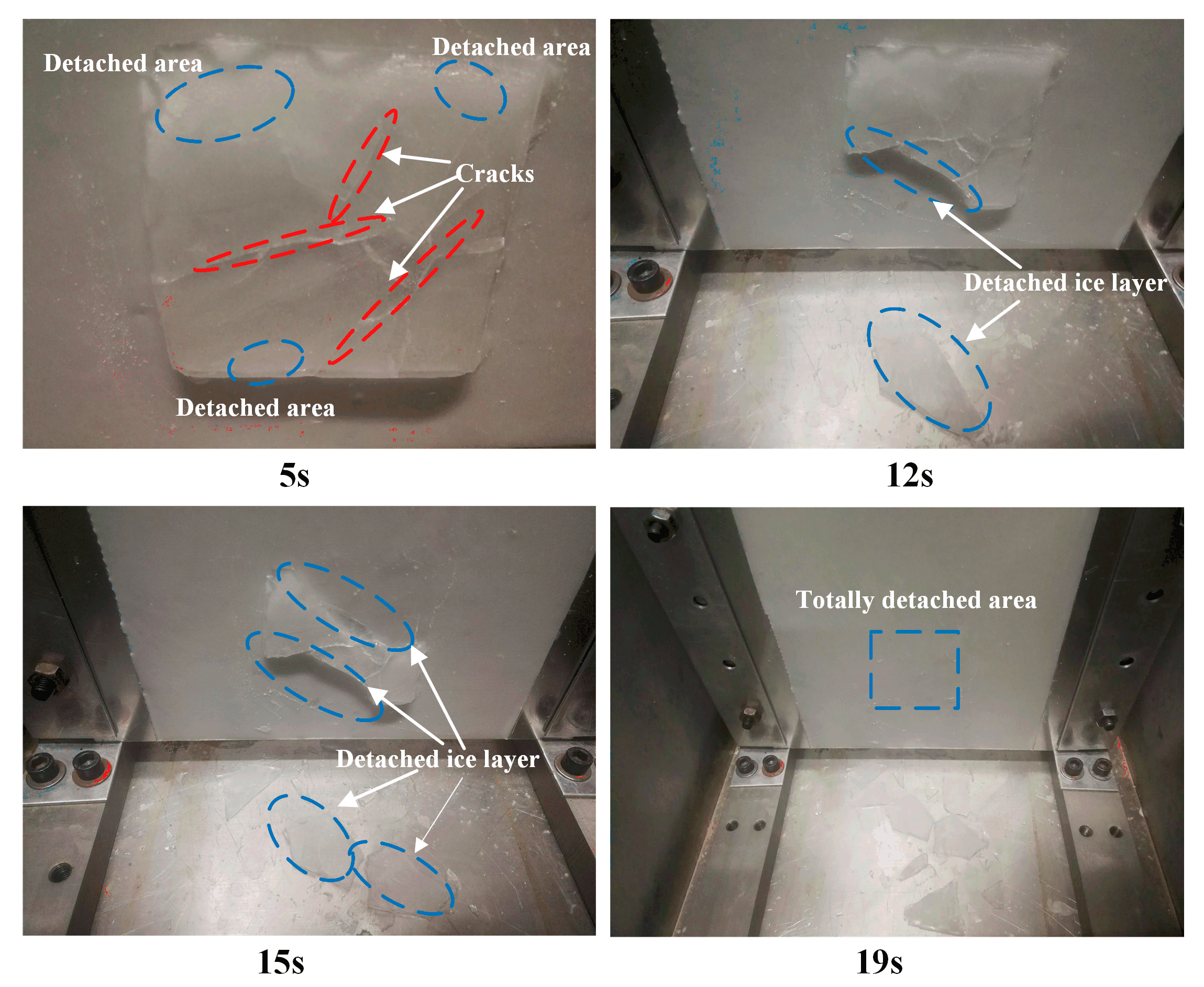
3.2. Experimental Validation

In this section, ultrasonic de-icing experiments are conducted to validate the analytical results above. These validations cannot only verify the applicability of proposed model, but also provide guidance for the further parametric design for the host plate-coating-ice layered structure to achieve de-icing more efficiently. In the process, the density and Poisson’s ratio are constant for a specific coating. Therefore, the experimental verifications mainly focus on the effects of the coating Young’s modulus, thickness, and ice layer thickness. Similarly, when verifying a certain parameter, the values of all other parameters are fixed.

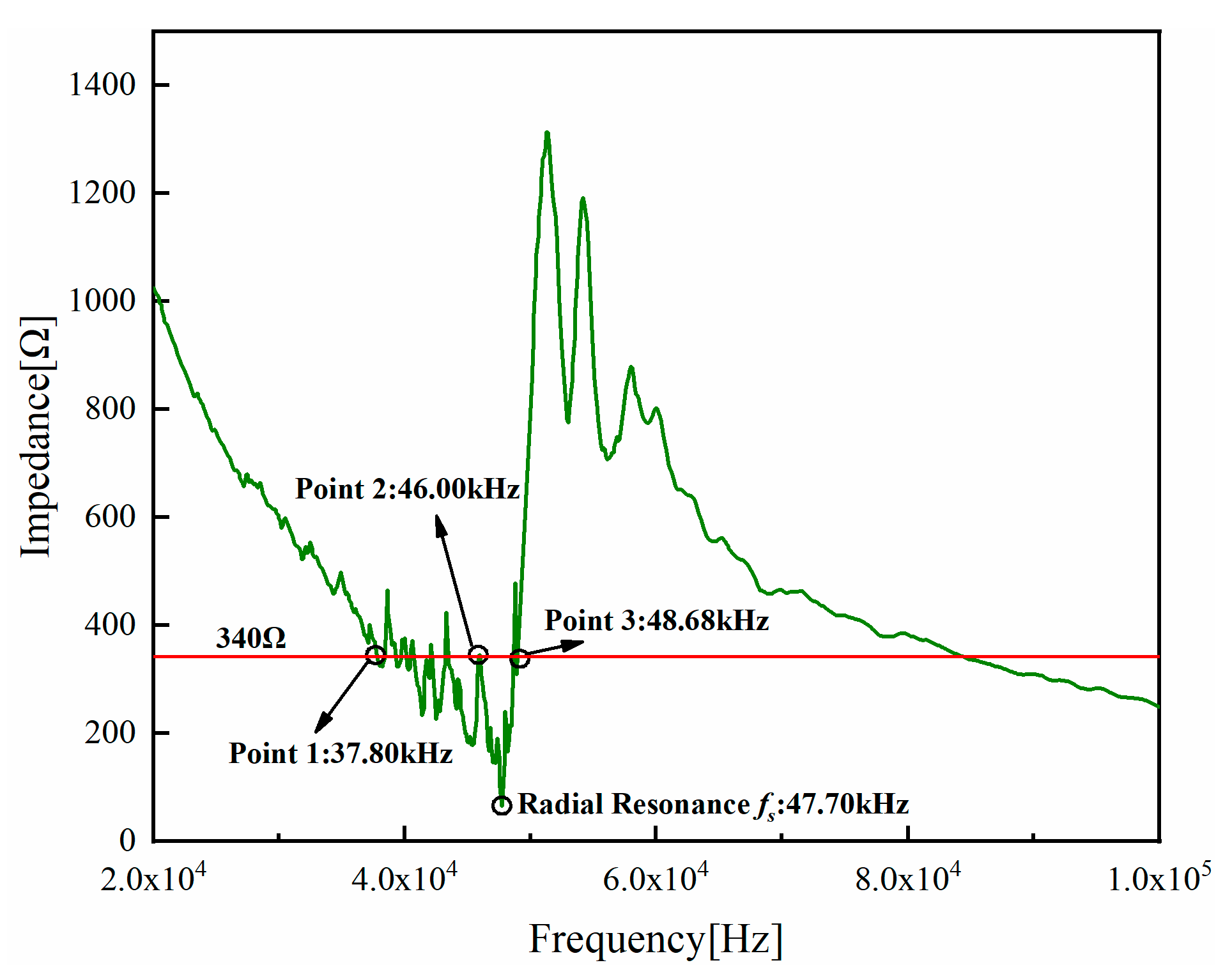
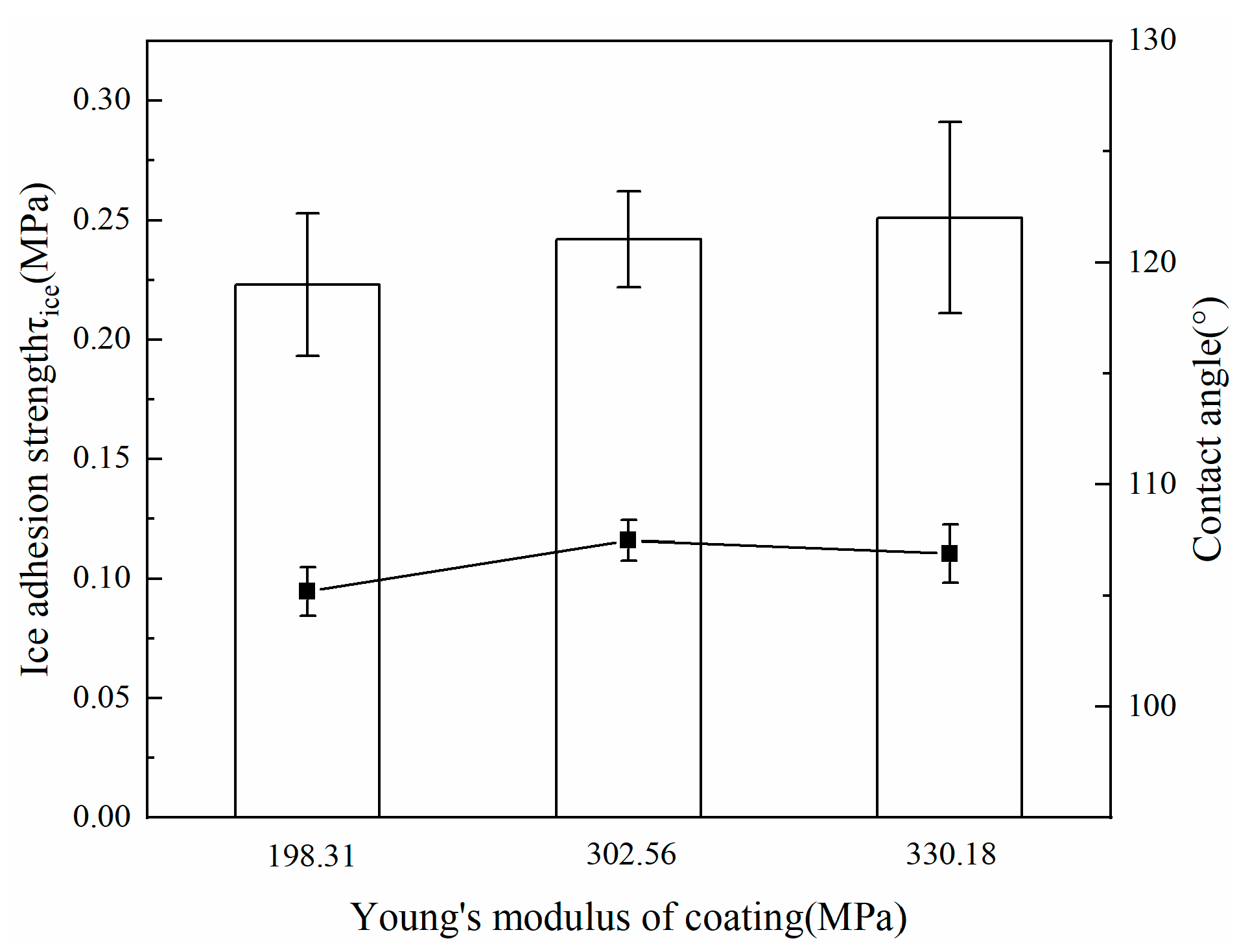
3.2.1. Verification of Young’s Modulus of the Coating

The dimensions of the specimen plate used in the experiment were 300 mm × 300 mm with a thickness of 2 mm. A 50-mm-diameter, 2.5-mm-thick PZT-4 actuator was attached on the back side of the plate, which was 60 mm away from the edge of the aluminum plate in the length direction of the coating. The coating used for anti-icing is made from epoxy, silicone rubber, and silicone oil. Coatings with different Young’s moduli can be obtained by changing the proportion of the component. A piece of ice layer (80 mm × 80 mm × 4 mm) was frozen on the center of the coatings. Experiments were performed at a temperature of −10 °C in the freezer.

Prior to de-icing, impedance curves of the PZT-4 disk bonded to the plate-coating-ice layered structure were measured using an impedance analyzer. Figure 11 presents the impedance curve when the coating Young’s modulus is 302.56 MPa. The radial resonant frequency of the PZT-4 actuator is 47.70 kHz. In addition, three frequency points (see Figure 11) with the same impedance of 340 Ω were selected as optimal frequencies to conduct de-icing experiments. Based on the optimal frequencies calculated above, the coating Young’s moduli were confirmed to be 198.31 MPa, 302.56 MPa, and 330.18 MPa, respectively. It is the same A₁ mode of Lamb waves to get the maximum ISCC values for these three coatings according to the results of Figure 5a. Given that the Young’s modulus and thickness of the coating may affect the adhesion strength between the ice layer and anti-icing coating [30], ice adhesion strengths were tested prior to the de-icing experiments. The detailed method for measuring the adhesion strength between the ice layer and these coatings can be found in Refs. [31,32,33]. Figure 12 presents the adhesion strength values and contact angles of various Young’s modulus coatings. The adhesion strengths were 0.223 ± 0.035, 0.242 ± 0.027, and 0.251 ± 0.041 MPa, respectively. The contact angles were 105.2° ± 1.1°, 107.5° ± 0.9°, and 106.9° ± 1.3°, respectively. There were no significant adhesion strength differences among the interfaces between the ice layer and coatings with different Young’s moduli. This phenomenon can be explained by the relatively high Young’s modulus of the coatings, which is referred to as hard coating.

The experimental setup and de-icing experimental schematic diagram are shown in Figure 13. The time of voltage applied to the PZT actuator is specified as 20 s. The de-icing time was set to 19 ± 1 s. When ice was totally removed from the coating within 19 ± 1 s, the voltage applied to the PZT actuator was recorded, otherwise the voltage would increase. As described before, de-icing frequency was confirmed after the impedance curve of the PZT actuator was measured.

The de-icing process for the coating with a Young’s modulus of 302.56 MPa is shown in Figure 14. The voltage applied was 248.4 V with a standard deviation of 8.6 V, at a frequency of 46.00 kHz. As the voltage was applied to the PZT actuator, the top and bottom edges of the ice layer started to detach from the coating after 5 s. Meanwhile, some cracks can be observed during the process. After 12 s, the bottom edges of the ice layer were partially peeled off with more cracks. After 15 s, ice detachment was observed at the top edge of the ice layer. The detached area continued to increase, and the center of the ice layer started to detach from the coating. Finally, the ice layer was completely removed at 19 s.

Similar experimental processes were conducted on the other coatings with different Young’s moduli. The frequencies of 37.80 kHz, 46.00 kHz, and 48.68 kHz were used for the coatings with the Young’s modulus of 198.31 MPa, 302.56 MPa, and 330.18 MPa, respectively. Each case was performed at least 5 times. Meanwhile, the maximum ISCC values were calculated for these three groups of coatings. As described before, the maximum ISCC value for Lamb waves is greater than that of the SH waves at the same material properties for this model. Therefore, only the maximum ISCC value for Lamb wave was presented here. The results are shown in Figure 15. The voltage applied to PZT disk for 198.31 MPa, 302.56 MPa and 330.18 MPa coatings were 215.8 ± 9.4, 248.4 ± 8.6 and 269.6 ± 12.1 V, respectively. The voltage was relatively high since the PZT disk didn’t work at its resonance frequency. Based on voltage, power consumed were estimated to be 135.2 ± 12.0, 175.7 ± 12.4 and 218.4 ± 20.0 W, respectively. ISCC values were calculated to be 0.3625, 0.3525 and 0.3518 $\mathrm{GPa}/\sqrt{\mathrm{GW}/\mathrm{m}}$ for these three groups of coatings. It can be founded that the de-icing power required increases and the maximum ISCC values decrease with an increase in the coating Young’s modulus. The trend of the maximum ISCC value coincides with the result of Figure 5a. According to the definition of ISCC, the experimental results agree well with analytical results. Considering the results above, it can be concluded that appropriately reducing the Young’s modulus of the coating is beneficial to de-icing.

3.2.2. Verification of Coating Thickness

In the de-icing process for the coating with a Young’s modulus of 330.18 MPa, the piezoelectric disk locally generated electric sparks and cracks when the voltage applied exceeded 300 V. Therefore, the three PZT actuators were redesigned and manufactured with the same diameter–thickness ratio to conduct the following de-icing experiments. The diameters for these three groups of designed actuators were 40 mm, 50 mm, and 60 mm; and the thicknesses were 2 mm, 2.5 mm, and 3 mm. These three groups of actuators were designed and used at their own resonant frequencies. The planar coupling factors k_p for these three actuators were 56.38%, 56.40%, and 56.34%, respectively, thus the de-icing power for these actuators was comparable. After they were bonded to a plate, the radial resonant frequencies were 57.6 kHz, 47.7 kHz, and 38.1 kHz, respectively. In the experiments, the Young’s modulus of the coatings was 198.31 MPa. The thickness of the ice layer was 1 mm. According to the calculated results, the thicknesses of the coatings were designed to be 0.42 mm, 0.63 mm, and 0.98 mm. It appears in A₁ mode of Lamb waves to obtain the maximum ISCC value for these three coatings according to the result of Figure 7a. The adhesion strengths and contact angles of ice on the coatings were tested and are shown in Figure 16. The adhesion strengths of coatings with the thicknesses of 0.42 mm, 0.63 mm, and 0.98 mm were 0.231 ± 0.033, 0.228 ± 0.041, and 0.223 ± 0.035 MPa, respectively. The contact angles were 106.5° ± 1.3°,107.2° ± 1.0°, and 105.2° ± 1.1° respectively. Considering these results, no apparent adhesion strength or contact angle differences were observed for these three groups of coatings.

Three group PZT disks were used on coatings with thicknesses of 0.42 mm, 0.63 mm, and 0.98 mm. Similar de-icing experiment processes were conducted for these three coatings as before. The results are shown in Figure 17. The voltage required to detach ice layers for these three coatings were 54.4 ± 6.2, 65.8 ± 5.8 and 75.1 ± 4.3 V, respectively. The power required to detach the ice layer from these three groups of coatings were 53.8 ± 12.9, 63.7 ± 11.7, and 97.2 ± 11.5 W, respectively. The maximum ISCC values were calculated for these three coatings. Similar as mentioned in Section 3.2.1, only the maximum ISCC value for Lamb waves was showed. ISCC values were calculated to be 0.3938, 0.3802 and 0.3627 $\mathrm{GPa}/\sqrt{\mathrm{GW}/\mathrm{m}}$. From these results, it can be found that the increases of coating thickness lead to the increase in both the voltage and power required for de-icing. This result also verified the trend of ISCC calculated shown in Figure 7a, which decreased with the increase in coating thickness. Thus, appropriately reducing the thickness of the coating is conducive to ultrasonic de-icing.

3.2.3. Verification of Ice Thickness

In this section, the effect of ice thickness on de-icing was analyzed. The coating Young’s modulus was 198.31 MPa (same as above) and the thickness was 0.63 mm. The thickness of ice layers was assigned to 1.9 mm, 4.0 mm, and 9.8 mm according to the calculation results. The optimal mode corresponding to these three different thickness ice layers is the A₁ mode of the Lamb waves. The three groups of designed PZT disks were used in the de-icing experiments with 1.9 mm, 4.0 mm, and 9.8 mm ice layers, respectively. As shown in Figure 18, the de-icing voltage and power consumed increases with an increase in the ice thickness. The voltage required to detach ice layers for these three coatings were 55.8 ± 5.5, 65.8 ± 5.8 and 78.9 ± 6.6 V, respectively. The power needed to detach 1.9 mm, 4.0 mm, and 9.8 mm ice layers were 55.6 ± 11.5, 63. 7 ± 11.7, and 122.1 ± 21.2 W, respectively. The maximum ISCC values for Lamb waves were calculated to be 0.4125, 0.3802, and 0.2885 $\mathrm{GPa}/\sqrt{\mathrm{GW}/\mathrm{m}}$, respectively. The experimental results agree with the prediction from the calculations. As indicated in the calculated results above, the ISCC value presents a non-monotonic behavior. When different thicknesses of ice layers correspond to the same mode in dispersion curve to obtain the maximum ISCC value, the ISCC value increases with the increase in ice thickness. Therefore, it can be concluded that it is feasible to reduce de-icing power by reasonable selection of ice thickness, especially with the icing monitoring method.

4. Conclusions

In this paper, a thorough parametric study of the ultrasonic de-icing method on a plate with coating was presented. A three-layer plate model (host plate-coating-ice) was investigated using global matrix method, cased on the theory of ultrasonic guided wave propagation in a multi-layered structure. Interface shear concentration coefficient (ISCC) was introduced to represent the ability of ultrasonic de-icing. The effects of the coating material parameters including Young’s modulus, thickness, density and Poisson’s ratio of coating and ice thickness on the ISCC values and optimal frequencies were analyzed. According to calculation results, more attention should be paid to Lamb waves for this model, because the ISCC values for Lamb waves are greater than those of SH waves at the same material properties. Subsequently, experiments were conducted, and validation of the de-icing effect of coating Young’s modulus, coating thickness, and ice thickness was executed according to the calculated results. The trends of power consumption and optimal frequency agreed with the calculated results. The results show that appropriately reducing the Young’s modulus of the coating can achieve de-icing with less power. When the strength and usability of the coating are satisfied, appropriately decreasing the thickness of the coating is conducive to de-ice. When different thicknesses of the ice layer correspond to the same optimal mode in the dispersion curves, more power is required to detach the thicker ice layers. Although, the effects of density and Poisson’s ratio of coating on de-icing were not validated in experiments, since these two parameters were constant for a specific coating. However, based on the experimental results of the remaining three parameters, the correctness and practical value of model proposed were validated. Therefore, the effects of density and Poisson’s ratio of coating calculated can also be the guidance in the design process of the coating.

References

1. Ryerson, C.C. Ice protection of offshore platforms. Cold Reg. Sci. Technol. 2011, 65, 97–110. [Google Scholar] [CrossRef]
2. Rashid, T.; Khawaja, H.A.; Edvardsen, K. Review of marine icing and anti-/de-icing systems. J. Mar. Eng. Technol. 2016, 15, 79–87. [Google Scholar] [CrossRef]
3. Saha, D. Experimental Investigation of On-Deck Icing for Marine Vessels. Ph.D. Thesis, Memorial University of Newfoundland, St. John’s, NL, Canada, 2017. [Google Scholar]
4. Sultana, K.; Dehghani, S.; Pope, K.; Muzychka, Y. A review of numerical modelling techniques for marine icing applications. Cold Reg. Sci. Technol. 2018, 145, 40–51. [Google Scholar] [CrossRef]
5. Wang, Z. Recent progress on ultrasonic de-icing technique used for wind power generation, high-voltage transmission line and aircraft. Energy Build. 2017, 140, 42–49. [Google Scholar] [CrossRef]
6. Wang, Y.; Xu, Y.; Huang, Q. Progress on ultrasonic guided waves de-icing techniques in improving aviation energy efficiency. Renew. Sustain. Energy Rev. 2017, 79, 638–645. [Google Scholar] [CrossRef]
7. Sundén, B.; Wu, Z. On icing and icing mitigation of wind turbine blades in cold climate. J. Energy Resour. Technol. 2015, 137, 051203. [Google Scholar] [CrossRef]
8. Shu, L.; Li, H.; Hu, Q.; Jiang, X.; Qiu, G.; He, G.; Liu, Y. 3D numerical simulation of aerodynamic performance of iced contaminated wind turbine rotors. Cold Reg. Sci. Technol. 2018, 148, 50–62. [Google Scholar] [CrossRef]
9. Solangi, A.R. Icing Effects on Power Lines and Anti-Icing and De-Icing Methods. Master’s Thesis, UiT The Arctic University of Norway, Tromsø, Norway, 2018. [Google Scholar]
10. Parent, O.; Ilinca, A. Anti-icing and de-icing techniques for wind turbines: Critical review. Cold Reg. Sci. Technol. 2011, 65, 88–96. [Google Scholar] [CrossRef]
11. Möhle, E.; Haupt, M.C.; Horst, P. Coupled numerical simulation and experimental validation of the electroimpulse de-icing process. J. Aircr. 2013, 50, 96–102. [Google Scholar] [CrossRef]
12. Budinger, M.; Pommier-Budinger, V.; Napias, G.; Costa da Silva, A. Ultrasonic Ice Protection Systems: Analytical and Numerical Models for Architecture Tradeoff. J. Aircr. 2016, 53, 680–690. [Google Scholar] [CrossRef] [Green Version]
13. Zhu, Y.; Palacios, J.; Rose, J.; Smith, E. De-icing of multi-layer composite plates using ultrasonic guided waves. In Proceedings of the 49th AIAA/ASME/ASCE/AHS/ASC Structures, Structural Dynamics, and Materials Conference, 16th AIAA/ASME/AHS Adaptive Structures Conference, 10th AIAA Non-Deterministic Approaches Conference, 9th AIAA Gossamer Spacecraft Forum, 4th AIAA Multidisciplinary Design Optimization Specialists Conference, Schaumburg, IL, USA, 7–10 April 2008. [Google Scholar] [CrossRef]
14. Tan, H.; Xu, G.; Tao, T.; Sun, X.; Yao, W. Experimental investigation on the defrosting performance of a finned-tube evaporator using intermittent ultrasonic vibration. Appl. Energy 2015, 158, 220–232. [Google Scholar] [CrossRef]
15. Gao, H.; Rose, J.L. Ice detection and classification on an aircraft wing with ultrasonic shear horizontal guided waves. IEEE Trans. Ultrason. Ferroelectr. Freq. Control 2009, 56, 334–344. [Google Scholar] [PubMed]
16. Ramanathan, S.; Varadan, V.V.; Varadan, V.K. Deicing of helicopter blades using piezoelectric actuators. In Proceedings of the Smart Structures and Materials 2000: Smart Electronics and MEMS, Newport Beach, CA, USA, 6–9 March 2000; pp. 281–292. [Google Scholar]
17. Palacios, J.; Smith, E.; Rose, J.; Royer, R. Instantaneous de-icing of freezer ice via ultrasonic actuation. AIAA J. 2011, 49, 1158–1167. [Google Scholar] [CrossRef] [Green Version]
18. Habibi, H.; Cheng, L.; Zheng, H.; Kappatos, V.; Selcuk, C.; Gan, T.-H. A dual de-icing system for wind turbine blades combining high-power ultrasonic guided waves and low-frequency forced vibrations. Renew. Energy 2015, 83, 859–870. [Google Scholar] [CrossRef] [Green Version]
19. Zhu, Y. Structural Tailoring and Actuation Studies for Low Power Ultrasonic De-Icing of Aluminum and Composite Plates. Ph.D. Thesis, The Pennsylvania State University, State College, PA, USA, 2010. [Google Scholar]
20. Kalkowski, M.K.; Rustighi, E.; Waters, T.P. Modelling piezoelectric excitation in waveguides using the semi-analytical finite element method. Comput. Struct. 2016, 173, 174–186. [Google Scholar] [CrossRef] [Green Version]
21. Kalkowski, M.K.; Waters, T.P.; Rustighi, E. Delamination of surface accretions with structural waves: Piezo-actuation and power requirements. J. Intell. Mater. Syst. Struct. 2017, 28, 1454–1471. [Google Scholar] [CrossRef]
22. Wang, Y.; Xu, Y.; Lei, Y. An effect assessment and prediction method of ultrasonic de-icing for composite wind turbine blades. Renew. Energy 2018, 118, 1015–1023. [Google Scholar] [CrossRef]
23. Daniliuk, V.; Xu, Y.; Liu, R.; He, T.; Wang, X. Ultrasonic de-icing of wind turbine blades: Performance comparison of perspective transducers. Renew. Energy 2020, 145, 2005–2018. [Google Scholar] [CrossRef]
24. Qian, H.; Xu, D.; Du, C.; Zhang, D.; Li, X.; Huang, L.; Deng, L.; Tu, Y.; Mol, J.M.; Terryn, H.A. Dual-action smart coatings with a self-healing superhydrophobic surface and anti-corrosion properties. J. Mater. Chem. A 2017, 5, 2355–2364. [Google Scholar] [CrossRef] [Green Version]
25. Cao, L.; Jones, A.K.; Sikka, V.K.; Wu, J.; Gao, D. Anti-icing superhydrophobic coatings. Langmuir 2009, 25, 12444–12448. [Google Scholar] [CrossRef]
26. Rose, J.L. Ultrasonic Guided Waves in Solid Media; Cambridge University Press: Cambridge, UK, 2014. [Google Scholar]
27. Giurgiutiu, V. Structural health monitoring (SHM) of aerospace composites. In Polymer Composites in the Aerospace Industry; Elsevier: Amsterdam, The Netherlands, 2020; pp. 491–558. [Google Scholar]
28. Palacios, J.; Zhu, Y.; Smith, E.; Rose, J. Ultrasonic shear and lamb wave interface stress for helicopter rotor de-icing purposes. In Proceedings of the 47th AIAA/ASME/ASCE/AHS/ASC Structures, Structural Dynamics, and Materials Conference 14th AIAA/ASME/AHS Adaptive Structures Conference 7th, Newport, RI, USA, 1–4 May 2006. [Google Scholar] [CrossRef]
29. Bocchini, P.; Marzani, A.; Viola, E. Graphical user interface for guided acoustic waves. J. Comput. Civ. Eng. 2011, 25, 202–210. [Google Scholar] [CrossRef]
30. Chaudhury, M.; Kim, K. Shear-induced adhesive failure of a rigid slab in contact with a thin confined film. Eur. Phys. J. E 2007, 23, 175–183. [Google Scholar] [CrossRef]
31. Xie, Q.; Hao, T.; Zhang, J.; Wang, C.; Zhang, R.; Qi, H. Anti-Icing Performance of a Coating Based on Nano/Microsilica Particle-Filled Amino-Terminated PDMS-Modified Epoxy. Coatings 2019, 9, 771. [Google Scholar] [CrossRef] [Green Version]
32. Guerin, F.; Laforte, C.; Farinas, M.-I.; Perron, J. Analytical model based on experimental data of centrifuge ice adhesion tests with different substrates. Cold Reg. Sci. Technol. 2016, 121, 93–99. [Google Scholar] [CrossRef]
33. Laforte, C.; Beisswenger, A. Icephobic material centrifuge adhesion test. In Proceedings of the 11th International Workshop on Atmospheric Icing of Structures, IWAIS, Montreal, QC, Canada, 13–16 June 2005; pp. 12–16. [Google Scholar]
Figure 1. Schematic of a general three-layer plate model.
Coatings 10 00631 g001
Figure 2. Dispersion curves of, (a) Lamb waves using GMM; (b) Lamb waves using SAFE; (c) SH waves using GMM; and (d) SH waves using SAFE.
Coatings 10 00631 g002
Figure 3. Wave structures of (a) S1 mode at 200 kHz; (b) SH3 mode at 300 kHz.
Coatings 10 00631 g003
Figure 4. Example of ISCC values superimposing on dispersion curves of SH waves (left) and Lamb waves (right), applying to three Young’s moduli of coating: (a) 20 MPa; (b) 50 MPa; (c) 500 MPa.
Coatings 10 00631 g004
Figure 5. Effect of Young’s modulus of coating on maximum ISCC value and optimal frequency: (a) Lamb waves; (b) SH waves.
Coatings 10 00631 g005
Figure 6. Shear stress (σ31) wave structure of Lamb waves corresponding to the maximum ISCC for different Young’s moduli of coating: (a) 0.8 MPa–40 MPa (all wave structures belong to S3 mode); (b) 50 MPa–100 MPa (all wave structures belong to the S2 mode); (c) 200 MPa–500 MPa (all wave structures belong to A1 mode).
Coatings 10 00631 g006
Figure 7. The effects of coating thickness on maximum ISCC value and optimal frequency: (a) Lamb waves; (b) SH waves.
Coatings 10 00631 g007
Figure 8. The effects of coating density on the maximum ISCC value and the optimal frequency: (a) Lamb waves; (b) SH waves.
Coatings 10 00631 g008
Figure 9. Effect of coating Poisson’s ratio on ISCC value and optimal frequency: (a) Lamb wave; (b) SH wave.
Coatings 10 00631 g009
Figure 10. The effects of ice thickness on maximum ISCC and optimal frequency: (a) Lamb wave; (b) SH wave.
Coatings 10 00631 g010
Figure 11. Impedance curve of PZT-4 bonded to a plate-coating-ice-layered structure.
Coatings 10 00631 g011
Figure 12. Adhesion strength and contact angle of different Young’s modulus coatings.
Coatings 10 00631 g012
Figure 13. Experimental setup and de-icing experimental schematic diagram.
Coatings 10 00631 g013
Figure 14. De-icing process for coating with Young’s modulus 302.56 MPa.
Coatings 10 00631 g014
Figure 15. De-icing voltage, power, and the maximum ISCC value for coatings with different Young’s moduli.
Coatings 10 00631 g015
Figure 16. Adhesion strength and contact angle for coatings with different thicknesses.
Coatings 10 00631 g016
Figure 17. De-icing voltage, power, and the maximum ISCC value for coatings with different thicknesses.
Coatings 10 00631 g017
Figure 18. De-icing voltage, power, and the maximum ISCC value for ice layers with varying thicknesses.
Coatings 10 00631 g018