Thermoelastic Response Induced by Volumetric Absorption of Uniform Laser Radiation in a Half-Space

Abstract

In this paper, the thermoelastic response in a generalized thermoelastic half-space induced by absorption of a penetrating pulsed laser radiation inside the medium is studied using the generalized theory with Dual-Phase-Lag (DPL). The surface of the target is considered stresses free and exposed to temperature-dependent heat losses. Laplace integral transform is used analytically for obtaining the general solution, while its inverse is carried out numerically. The copper element is used as an application to compare the predictions induced by volumetric absorption of the Dual-Phase-lag theory with those for Lord–Shulman (LS) and classical coupled (CTE) theories, moreover the response induced by volumetric absorption for (LS) and (CTE) models in this work were compared with those induced by surface absorption in a previous work.

1. Introduction

A rapid growth in scientific research of the thermoelasticity field was observed after Biot (1956) [1] introduced the coupled theory of thermoelasticity (CTE) to fade the flaws of the classical uncoupled theory, stating that the elastic disturbance has no influence on temperature and the temperature waves travel with infinite speeds. Although this theory repairs the first defect by coupling between temperature and strain, the energy equation of this theory was based on Fourier’s law and, thus, its heat waves still travel with infinite speed. Employing Biot’s model Hetnarski [2,3] has discussed some remarkable problems in this direction. Furthermore, the work done by Boley and Tolins [4] considered a good contribution.

The defect of the infinite speed in Biot’s theorem was eliminated by the generalization introduced by Lord and Shulman in 1967, this generalization was known as the generalized theory of thermoelasticity with one relaxation time (LS) [5]. The energy equation of the latter theory was constructed on a new law of heat conduction instead of Fourier’s law and, thus, the defect of infinite speed was repaired. As significant contributions in the context of this theory, we mention the proofs of uniqueness theorems under different conditions by Ignaczak [6,7]. Furthermore, Sherief el al. [8,9,10] obtained solutions of some thermoelastic problems by employing Lord and Shulman’s theory.

Many models such as [11,12,13] have been introduced to be generalizations to Biot’s theory, in which the generated heat waves travel with finite speeds. One of the substantial models was the generalized theory with dual-phase-lag (DPL), which was developed by Ozisik and Tzou [14] and Tzou [15,16]. In this model, Fourier’s law was replaced by an approximation that includes two distinct time translations signifying the phase lags of temperature gradient and heat flux. RoyChoudhuri [17] employed the DPL model to study the disturbances in an elastic 1D half-space subjected to two different boundary conditions. Using the DPL model, Aboelregal [18] obtained the solution of a 1D semi-infinite medium whose boundary plane was exposed to thermal shock. EL-Karamany and Ezzat [19] published a considerable study on the Dual-Phase-Lag model. Abbas and Zenkour [20] studied the dual-phase-lag model on thermoelastic interactions in a half-space exposed to a ramp-type heating by applying the finite element method. Marin et al. [21] studied the well-posed dual-phase-lag model of a thermoelastic dipolar material.

One of the significant sources leading to thermal influences is the pulsed laser, which gives a high density in small periods of time and this, in turn, yields a great importance economically. Since lasers were founded, many applications have been made in science, mechanics and engineering based on their specific properties [22]. Many theoretical studies have been conducted to study thermoelastic responses induced by laser radiation [23,24,25]. Henain et al. [26] studied the surface illumination of a 2D thermoelastic homogeneous semi-infinite medium. Yossef and EL-Bary [27] applied four thermoelastic theories to study the response in an elastic half-space induced by laser pulse whose temporal profile is non-Gaussian. Allam and Tayel [28] obtained a solution for a 1D thermoelastic functionally graded half-space heated uniformly by a surface absorption of pulsed laser having Gaussian temporal profile. Abbas and Marin [29] studied the thermoelastic interaction induced by laser pulse in a 2D half-space and introduced an analytical solution in the context of the generalized theory with one relaxation time. Tayel and Hassan [30] employed the fractional order theory of thermoelasticity to study the effect of the fractional parameter in the existence and absence of heat losses in a thermoelastic half-space heated uniformly by surface absorption of laser radiation.

The aims of this work are to investigate the thermoelastic interactions in a half-space induced by volumetric absorption of laser radiation in the existence and absence of heat losses by employing three different theories of thermoelasticity, namely, DPL, LS, and CTE, and to study the influences of the phase lag of the temperature gradient of the dual-phase-lag theory. Moreover, the response of LS and CTE models will be compared with the response induced by surface absorption technique in a previously published paper [30].

2. Problem Formulation and Basic Equation

We consider a laser beam to be incident uniformly in z-direction perpendicular to a homogeneous and isotropic thermoelastic half-space $(z⩾0)$ whose initial temperature is $T_0$. The irradiated surface $(z=0)$ is taken to be traction free and subjected to heat losses whose coefficient is temperature-dependent. At the irradiated surface, a part of the laser radiation will be reflected, while the rest will be absorbed into the medium to be converted into heat and, consequently, thermoelastic waves will be generated.

Due to the uniform illumination of the surface $(z=0)$, the problem will be 1D and all studied fields will be functions of z and t only, and consequently, the displacement vector $\mathbf{u}$ will have one component, namely $w(z,t)$, while the other components are vanishing.

Following the Dual-Phase-Lag theory (DPL) [15,16], the equations governing the thermoelastic waves in the absence of body forces for a one-dimensional problem are

• The heat conduction equation:

$$k\left(1+{\tau }_1\frac{\partial }{\partial t}\right)\frac{{\partial }^{2}T}{\partial z^2}=\left(1+{\tau }_2\frac{\partial }{\partial t}\right)\left(\rho C_E\frac{\partial T}{\partial t}+T_0\gamma \frac{{\partial }^{2}w}{\partial t\partial z}-Q\right).$$

(1)

where $T,k,\rho ,c_E,Q,T_0$ stand for the absolute temperature, thermal conductivity, denisty, specific heat at costant strain, heat source per unit volume, and reference temperature, which chosen such that $|(T-T_0)/T_0|\ll 1$. Furthermore, $\gamma =(3\lambda +2\mu ){\alpha }_T$, in which $\lambda$ and $\mu$ are Lamé’s constant and ${\alpha }_T$ is the coefficient of linear thermal expansion. ${\tau }_1$ and ${\tau }_2$ are the phase lag of the temperature gradient and heat flux, respectively, where $(0\le {\tau }_1<{\tau }_2)$.

The energy equations of LS and CTE models can be generated from Equation (1) by setting ${\tau }_1=0$ and ${\tau }_1={\tau }_2=0$, respectively.

• According to the volumetric absorption technique, the heat source, $Q(z,t)$ takes the form:

$$Q(z,t)=A_0{q}_{0}g\left(t\right)\xi e^{-\xi z}.$$

(2)

where $A_0$ is the transition coefficient of the irradiated surface, $\xi$ is the linear absorption coefficient of the material, $q_0$ is the maximum value of the laser power density and $g\left(t\right)$ is the time dependent laser pulse profile.

Using Equation (2), Equation (1) can be written as

$$k\left(1+{\tau }_1\frac{\partial }{\partial t}\right)\frac{{\partial }^{2}T}{\partial z^2}=\left(1+{\tau }_2\frac{\partial }{\partial t}\right)\left(\rho C_E\frac{\partial T}{\partial t}+T_0\gamma \frac{{\partial }^{2}w}{\partial t\partial z}-A_0{q}_{0}g\left(t\right)\xi e^{-\xi z}\right).$$

(3)

• The equation of motion:

$$\frac{\partial {\sigma }_{zz}}{\partial z}=\rho \frac{{\partial }^{2}w(z,t)}{\partial t^2}.$$

(4)

where ${\sigma }_{zz}$ is the normal stress.

For a 1D problem, the strain components are

$$e_{zz}=\frac{\partial w}{\partial z},e_{xx}=e_{yy}=e_{zx}=e_{zy}=e_{xy}=0.$$

(5)

Thus, the volume dilatation will be

$$e=e_{zz}+e_{xx}+e_{yy}=\frac{\partial w}{\partial z}.$$

(6)

The non-vanishing stresses are:

$$\begin{array}{cc}\hfill {\sigma }_{zz}& =2\mu \frac{\partial w}{\partial z}+\lambda e-\gamma \theta ,\hfill \end{array}$$

(7a)

$$\begin{array}{cc}\hfill {\sigma }_{xx}& =\lambda \frac{\partial w}{\partial z}-\gamma \theta ,\hfill \end{array}$$

(7b)

$$\begin{array}{cc}\hfill {\sigma }_{yy}& ={\sigma }_{xx}.\hfill \end{array}$$

(7c)

where $\theta =T-T_0$ is the temperature increment.

Using Equation (7a), Equation (4) can be written as

$$(\lambda +2\mu )\frac{{\partial }^{2}w}{\partial z^2}-\gamma \frac{\partial \theta }{\partial z}=\rho \frac{{\partial }^{2}w}{\partial t^2}.$$

(8)

Now, the boundary conditions can be expressed as:

$$\begin{array}{cc}\hfill k\left(1+{\tau }_1\frac{\partial }{\partial t}\right)\frac{\partial \theta }{\partial z}{|}_{z=0}& =\left(1+{\tau }_2\frac{\partial }{\partial t}\right)h\theta (0,t),\hfill \end{array}$$

(9a)

$$\begin{array}{cc}\hfill {\sigma }_{zz}{|}_{z=0}& =0,\hfill \end{array}$$

(9b)

$$\begin{array}{c}\hfill \theta ,w,{\sigma }_{zz}\to 0asz\to \infty .\end{array}$$

(9c)

where $\theta (0,t)$ is the surface temperature and h is the heat transfer coefficient.

Also, the initial conditions are:

$$\left.\begin{array}{cccccc}\hfill \theta (z,t){|}_{t=0}& =\frac{\partial \theta (z,t)}{\partial t}{|}_{t=0}\hfill & \hfill =0,& w(z,t){|}_{t=0}\hfill & \hfill =\frac{\partial w(z,t)}{\partial t}{|}_{t=0}& =0\hfill \\ \hfill {\sigma }_{ij}(z,t){|}_{t=0}& =\frac{\partial {\sigma }_{ij}(z,t)}{\partial t}{|}_{t=0}\hfill & \hfill =0.\end{array}\right\}$$

(10)

For simplicity, we introduce the following non-dimensional variables:

$$\begin{array}{cccccc}\hfill (z^{*},w^{*})& =(z,w)c\eta \hfill & \hfill {\theta }^{*}& =\frac{\gamma \theta }{(\lambda +2\mu )}\hfill & \hfill {\xi }^{*}& =\frac{\xi }{c\eta }\hfill \\ \hfill (t^{*},{\tau }_{1,2}^{*})& =(t,{\tau }_{1,2})c^2\eta \hfill & \hfill q_0^{*}& =\frac{\gamma q_0}{(\lambda +2\mu )c\rho C_E}\hfill & \hfill h^{*}& =\frac{h}{c\rho C_E}\hfill \\ \hfill {\sigma }_{ij}^{*}& =\frac{{\sigma }_{ij}}{\mu }\hfill & \hfill c& =\sqrt{\frac{\lambda +2\mu }{\rho }}\hfill & \hfill \eta & =\frac{\rho C_E}{k}.\hfill \end{array}$$

Making use of the non-dimensional variables after dropping the stars, Equations (3), (8) and (7) can be written respectively as:

$$\left(1+{\tau }_1\frac{\partial }{\partial t}\right)\frac{{\partial }^2\theta }{\partial z^2}=\left(1+{\tau }_2\frac{\partial }{\partial t}\right)\left(\frac{\partial \theta }{\partial t}+ϵ\frac{{\partial }^{2}w}{\partial t\partial z}-A_0{q}_0\xi e^{-\xi z}g\left(t\right)\right).$$

(11)

$$\frac{{\partial }^{2}w}{\partial z^2}-\frac{\partial \theta }{\partial z}=\frac{{\partial }^{2}w}{\partial t^2}.$$

(12)

$$\begin{array}{cc}\hfill {\sigma }_{zz}& =g_1\left(\frac{\partial w}{\partial z}-\theta \right),\hfill \end{array}$$

(13a)

$$\begin{array}{cc}\hfill {\sigma }_{xx}& =g_2\frac{\partial w}{\partial z}-g_1\theta ,\hfill \end{array}$$

(13b)

$$\begin{array}{cc}\hfill {\sigma }_{xx}& ={\sigma }_{yy}.\hfill \end{array}$$

(13c)

where

$$ϵ=\frac{{\gamma }^2{T}_0}{\rho C_E(\lambda +2\mu )},g_1=\frac{\lambda +2\mu }{\mu },g_2=\frac{\lambda }{\mu }.$$

The non-dimensional form of (9) is given as:

$$\begin{array}{cc}\hfill \left(1+{\tau }_1\frac{\partial }{\partial t}\right)\frac{\partial \theta }{\partial z}{|}_{z=0}& =\left(1+{\tau }_2\frac{\partial }{\partial t}\right)h\theta (0,t),\hfill \end{array}$$

(14a)

$$\begin{array}{cc}\hfill {\sigma }_{zz}{|}_{z=0}& =0,\hfill \end{array}$$

(14b)

$$\begin{array}{c}\hfill \theta ,w,{\sigma }_{zz}\to 0asz\to \infty .\end{array}$$

(14c)

3. Problem Solution

Introducing the Laplace integral transform with respect to the time [31]:

$$\tilde{f}(z,s)={\int }_0^{\infty }f(z,t)e^{-st}dt.$$

(15)

where $\tilde{f}(z,s)$ is the Laplace transform of $f(z,t)$ and s is the temporal angular frequency.

Applying (15) on Equations (11) and (12), one gets respectively

$$(D^2-\mathsf{\Lambda }s)\tilde{\theta }-ϵs\mathsf{\Lambda }D\tilde{w}=-A_0{q}_0\mathsf{\Lambda }\xi e^{-\xi z}\tilde{g}\left(s\right).$$

(16)

$$(D^2-s^2)\tilde{w}-D\tilde{\theta }=0.$$

(17)

where $\mathsf{\Lambda }=\frac{(1+{\tau }_{2}s)}{(1+{\tau }_{1}s)}$ and $\tilde{g}\left(s\right)$ is the Laplace transform of $g\left(t\right)$.

Applying the operator $(D^2-s^2)$ on Equation (16) and $ϵs\mathsf{\Lambda }D$ on Equation (17) then adding, one obtains the following fourth-order nonhomogeneous differential equation

$$(D^4-(s^2+s\mathsf{\Lambda }(1+ϵ))D^2+s^3\mathsf{\Lambda })\tilde{\theta }=-A_0{q}_0\mathsf{\Lambda }\xi ({\xi }^2-s^2)e^{-\xi z}\tilde{g}\left(s\right).$$

(18)

The last equation possesses the following characteristic equation

$$m^4-b_1\left(s\right)m^2+b_2\left(s\right)=0.$$

(19)

where $b_1\left(s\right)=s^2+s\mathsf{\Lambda }(1+ϵ)$ and $b_2\left(s\right)=s^3\mathsf{\Lambda }$.

It follows from Equation (18), that

$$(D^2-m_1^2)(D^2-m_2^2)\tilde{\theta }=-A_0{q}_0\mathsf{\Lambda }\xi ({\xi }^2-s^2)e^{-\xi z}\tilde{g}\left(s\right).$$

(20)

where $m_i^2,(i=1,2)$ are the roots of Equation (19), in which:

$$m_i^2=\frac{s^2+s\mathsf{\Lambda }(1+ϵ)\pm \sqrt{{(s^2+s\mathsf{\Lambda }(1+ϵ))}^2-4s^3\mathsf{\Lambda }}}{2}.$$

(21)

with the aid of the undermined coefficients method, the general solution of (20) is found to be

$$\tilde{\theta }=\sum _{i=1}^2{B}_i\left(s\right)e^{-m_{i}z}+H\left(s\right)e^{-\xi z},$$

(22)

with:

$$H=\frac{-A_0{q}_0\mathsf{\Lambda }\xi ({\xi }^2-s^2)\tilde{g}\left(s\right)}{({\xi }^2-m_1^2)({\xi }^2-m_2^2)}.$$

(23)

Following a similar manner to obtain $\tilde{w}$, it follows

$$(D^2-m_1^2)(D^2-m_2^2)\tilde{w}=A_0{q}_0\mathsf{\Lambda }{\xi }^2{e}^{-\xi z}\tilde{g}\left(s\right).$$

(24)

Solving Equation (24), one gets

$$\tilde{w}=\sum _{i=1}^2{N}_i\left(s\right)e^{-m_{i}z}+G\left(s\right)e^{-\xi z},$$

(25)

with

$$G\left(s\right)=\frac{A_0{q}_0\mathsf{\Lambda }{\xi }^2\tilde{g}\left(s\right)}{({\xi }^2-m_1^2)({\xi }^2-m_2^2)}.$$

(26)

Substituting for $\tilde{w}$ and $\tilde{\theta }$ in Equation (17), we obtain:

$$\begin{array}{cc}\hfill N_i\left(s\right)& =\frac{-m_i}{m_i^2-s^2}{B}_i\left(s\right)(i=1,2),\hfill \end{array}$$

(27a)

$$\begin{array}{cc}\hfill G\left(s\right)& =\frac{-\xi }{{\xi }^2-s^2}H\left(s\right).\hfill \end{array}$$

(27b)

Consequently, we can write

$$\tilde{w}=-\sum _{i=1}^2\left(\frac{m_i}{m_i^2-s^2}\right)B_i\left(s\right)e^{-m_{i}z}-\left(\frac{\xi }{{\xi }^2-s^2}\right)H\left(s\right)e^{-\xi z}.$$

(28)

Applying (15) on Equation (13), then substituting for $\tilde{\theta }$ and $\tilde{w}$, one find:

$$\begin{array}{cc}\hfill {\tilde{\sigma }}_{zz}& =g_1\left[\left(\frac{m_i^2}{m_i^2-s^2}-1\right)B_i\left(s\right)e^{-m_{i}z}+\left(\frac{{\xi }^2}{{\xi }^2-s^2}-1\right)H\left(s\right)e^{-\xi z}\right],\hfill \end{array}$$

(29a)

$$\begin{array}{cc}\hfill {\tilde{\sigma }}_{xx}& =\left[\left(g_2\frac{m_i^2}{m_i^2-s^2}-g_1\right)B_i\left(s\right)e^{-m_{i}z}+\left(g_2\frac{{\xi }^2}{{\xi }^2-s^2}-g_1\right)H\left(s\right)e^{-\xi z}\right],\hfill \end{array}$$

(29b)

$$\begin{array}{cc}\hfill {\tilde{\sigma }}_{xx}& ={\tilde{\sigma }}_{yy}.\hfill \end{array}$$

(29c)

By Applying (15) on (14) and using Equations (22) and (29a), one gets:

$$\begin{array}{cc}\hfill -\sum _{i=1}^2{m}_i{B}_i& =\xi H\left(s\right)+\mathsf{\Lambda }h\tilde{\theta }(0,s),\hfill \end{array}$$

(30a)

$$\begin{array}{cc}\hfill \sum _{i=1}^2{f}_i{B}_i& =-\mathsf{\Omega }H\left(s\right).\hfill \end{array}$$

(30b)

with

$$\mathsf{\Omega }=\frac{{\xi }^2}{{\xi }^2-s^2}-1,f_i=\frac{m_i^2}{m_i^2-s^2}-1,(i=1,2)$$

where $\tilde{\theta }(0,s)$ is the Laplace transform of $\theta (0,t)$.

Solving Equations (30a) and (30b) for $B_i,(i=1,2)$, one obtains:

$$\begin{array}{cc}\hfill B_1& =\frac{(h\mathsf{\Lambda }\tilde{\theta }(0,s)+H\xi )f_2-H\mathsf{\Omega }{m}_2}{-f_2{m}_1+f_1{m}_2},\hfill \end{array}$$

(31a)

$$\begin{array}{cc}\hfill B_2& =\frac{-(h\mathsf{\Lambda }\tilde{\theta }(0,s)+H\xi )f_1+H\mathsf{\Omega }{m}_1}{-f_2{m}_1+f_1{m}_2}.\hfill \end{array}$$

(31b)

Equations (31) contains $\tilde{\theta }(0,s)$, which still un-known, to complete the solution we shall substitute $B_1$ and $B_2$ in (22), one gets after setting $z=0$, the following equation:

$$\tilde{\theta }(0,s)=\frac{H(f_2(\xi -m_1)+f_1(m_2-\xi )+\mathsf{\Omega }(m_1-m_2))}{-f_2(h\mathsf{\Lambda }+m_1)+f_1(h\mathsf{\Lambda }+m_2)}.$$

(32)

4. Inverse Laplace Transformation

The formulas in Equations (22), (28) and (29) and the roots in Equation (21) predict great difficulties to be converted into the time domain by the usual analytical methods. So, the idea of utilizing a numerical methods will be acceptable to obtain inverse Laplace transform. Following [16], the method of Riemann-sum approximation, with $\eta t=4.7$ will be adopted using the following formula:

$$f\left(t\right)=\frac{e^{\eta t}}{t}\left[\frac{1}{2}\tilde{f}\left(\eta \right)+Re\sum _{n=1}^K{(-1)}^n\tilde{f}\left(\eta +\frac{in\pi }{t}\right)\right].$$

(33)

where K represents the number of terms, which should be sufficiently large and i is the imaginary unit numper.

5. Application and Computation

To demonstrate the consistency of the obtained results, an illustrative example is given for a copper half-space whose surface is illuminated by a pulsed laser assuming that ${\tau }_2=75\times {10}^{-5}$ and $\xi ={10}^5{m}^{-1}$. In order to compare the results of the present paper with those considered the surface absorption, the optical and physical parameters have to be used as [30]:

$$\begin{array}{cccccc}\hfill \rho & =8954kg/m^3\hfill & \hfill \lambda & =7.76\times {10}^{10}kg/(m.s^2)\hfill & \hfill \mu & =3.86\times {10}^{10}kg/(m.s^2)\hfill \\ \hfill C_E& =383.1J/(kg.K)\hfill & \hfill T_0& =293K\hfill & \hfill {\alpha }_T& =1.78\times {10}^{-5}{K}^{-1}\hfill \\ \hfill k& =386W/(m.K)\hfill & \hfill t_0& =3\times {10}^{-3}s\hfill & \hfill \delta & ={10}^{-3}s\hfill \\ \hfill h& =200W/(m^2.K)\hfill & \hfill q_0& ={10}^{4}W/m^2\hfill & \hfill A_0& =0.01.\hfill \end{array}$$

Consider the time dependent laser pulse profile $g\left(t\right)$ to be given by a Gaussian distribution as:

$$g\left(t\right)=e^{-{\left(\frac{t-t_0}{\delta }\right)}^2}.$$

(34)

where $\delta$ is the moment at which the laser beam intensity is reduced to $\frac{1}{e}$ and $t_0$ is the moment at which $g\left(t\right)$ becomes maximum.

6. Results

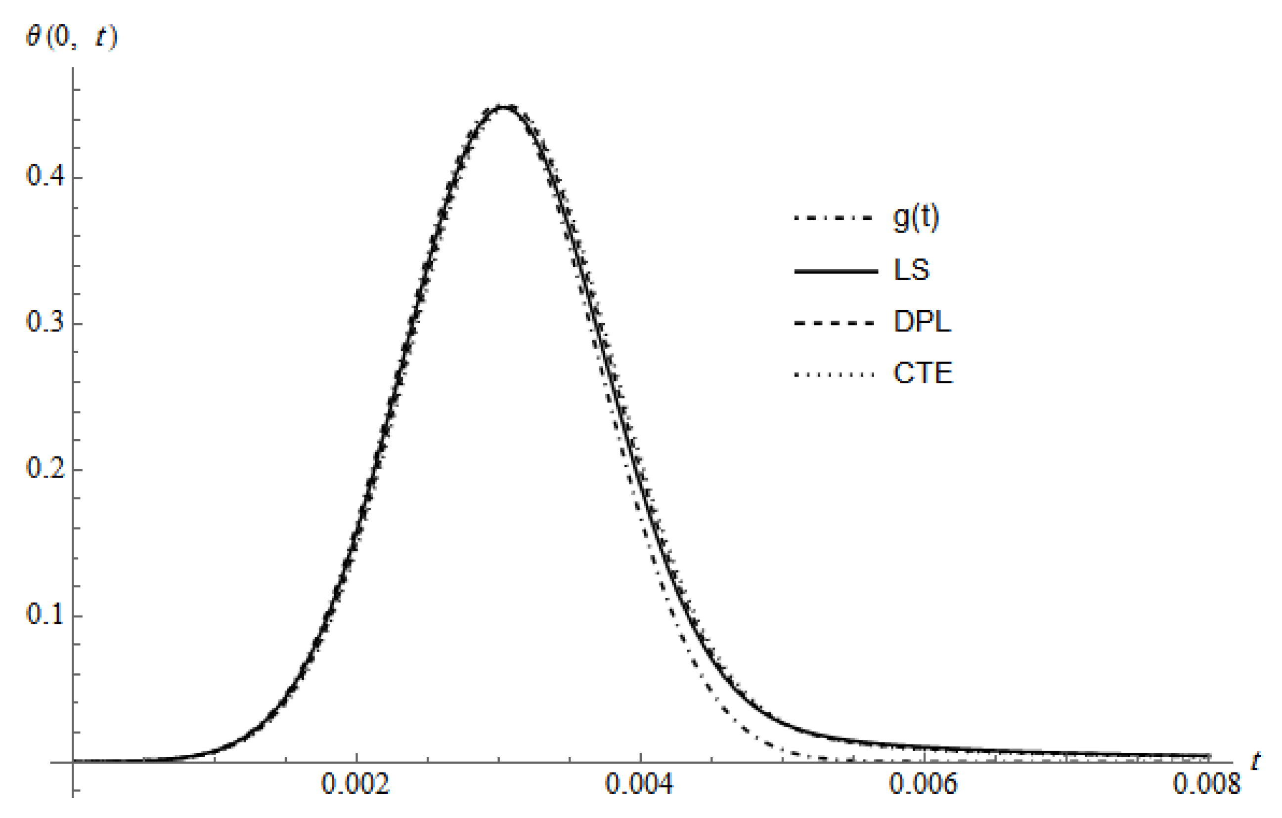
Figure 1 represents beside the curve of the chosen pulse profile $g\left(t\right)$, the time dependent surface temperature $\theta (0,t)$ for three different theories, namely LS, DPL and CTE calculated for $h=0$, the DPL curve calculated for ${\tau }_1=30\times {10}^{-5}$. The curves show, $\theta (0,t)$ increases with increasing the exposure time until the temperature reaches its maximum and then begins to decrease. This behavior can be interpreted as follows: at the beginning of the irradiation process, the conversion rate of the absorbed energy into heat is greater than the rate of the conducted one to the surrounding; this leads to piling up the heat energy in the vicinity of the illuminated surface and, thus, temperature rise. The increment of $\theta (0,t)$ is continued until the converted heat energy becomes equivalent to the conducted one; at this moment, the temperature reaches its maximum. After that, the absorbed energy begins to decrease and thus the conduction becomes greater than the absorption leading to decrease the temperature. As seen, the maximum value of the surface temperature is greater in the case of the generalized theories of LS and DPL than the case of the classical coupled theory of CTE. For the three curves, the maximum is shifted to greater times than the maximum of $g\left(t\right)$, but the CTE needs more time than the other theories to reach its maximum. The observed behavior can be interpreted as follows: beside the infinite speed of the heat waves of the CTE model, which leads to deeper spread of the temperature inside the medium, two different phenomena affect the spatial and temporal temperature distribution, namely, the heat conductivity described by the gradient of the temperature and the expansion of the material. While the first leads to heating the surroundings, the second will consume the heat energy in expanding the distances between particles and, thus, its potential energy increases. As observed in a later figure the CTE model having the greater spreading and the greater gradient of the spatial temperature close to the irradiated surface, so it has the smallest surface temperature. Since the maximum temperature occurs as the absorbed energy is equal to the consumed one, the LS and DPL maximum must occur more near the maximum of the laser profile $g\left(t\right)$ than that of the CTE, which consumes more energy in penetrating more into the medium. According to [30], the maximum values of $\theta (0,z)$ for the models of CTE and LS induced by the surface absorption is greater than the case of the volumetric absorption by approximately $20\%$ and its shift towards t-values is less.

Figure 2 represents $\theta (0,t)$ of the three theories LS, DPL and CTE calculated for $h\ne 0$, the DPL curve calculated for ${\tau }_1=30\times {10}^{-5}$. The figure shows a different behavior from Figure 1, where the three curves almost match with the curve of the pulse profile $g\left(t\right)$; this behavior is due to the conductivity of the martial together with the cooling effect. As in Figure 1, the curves of LS and CTE induced by volumetric absorption are smaller than the curves of the surface absorption [30].

Figure 3 represents $\theta (0,t)$ of the DPL model calculated for $h=0$ and different values of ${\tau }_1$ at a fixed value of ${\tau }_2$. The figure indicates that as ${\tau }_1$ takes value near ${\tau }_2$, $\theta (0,t)$ behaves approximately like the classical coupled theory (CTE) and as ${\tau }_1$ takes values far from ${\tau }_2$, $\theta (0,t)$ behaves approximately as the generalized theories in which this behavior is valid until a certain value approximately ${\tau }_1=1\times {10}^{-5}$ after this value the curves will be coincided for any values of ${\tau }_1$. The figure shows also that as ${\tau }_1$ decreases, the maximum of $\theta (0,t)$ increases. After $\theta (0,t)$ reaches its maximum value the slop of the curves are inverted with respect to the slop before the maximum value.

Figure 4 illustrates the spatial distribution of the temperature of the DPL model calculated for $h=0$ and ${\tau }_1=30\times {10}^{-5}$ at several times. The curves reveal a clear finite velocity which appears through the strong gradient at diverse locations and the increasing deep penetration as the time increase. The figure agrees with Figure 1, where its maximum temperature is located at the irradiated surface and occurs at a time greater than the time of the pulse profile $g\left(t\right)$. After the time at which the temperature reaches its maximum ($t=3.4\times {10}^{-3}$), a small gradient near the irradiated surface is observed owing to the decay of the absorbed energy inside the medium.

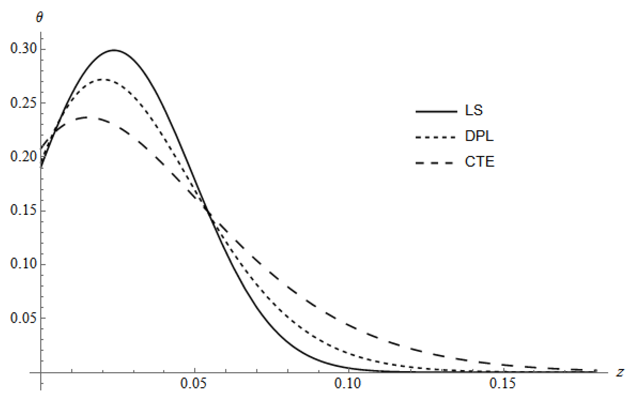
Figure 5 illustrates the spatial distribution of the temperature of three different models, LS, DPL and CTE, calculated for $h=0$ and $t=4\times {10}^{-3}$, the DPL curve calculated for ${\tau }_1=30\times {10}^{-5}$. The figure shows that the CTE model penetrates into the medium more than the other models (DPL and LS) and has the greatest gradient in the vicinity of the irradiated surface. This behavior is due to its infinite velocity of propagation. As seen, the maximum temperature of the LS model is smaller than the maximum of the other models and occurs near the surface of the target. This behavior is due to its relatively greater displacement at the irradiated surface which can be seen clearly in a later figure. This leads to store the heat energy in a mechanical potential energy and, therefore, slightly cools the surface due to heat conduction. Furthermore, the DPL model appears as a case between the LS and CTE. For the CTE and LS in the case of volumetric absorption, the temperature is smaller and the penetration depth is greater compared with the corresponding case of the surface absorption [30].

Figure 6 illustrates the spatial distribution of the temperature of the three different models (LS, DPL, and CTE) calculated for $h\ne 0$ at $t=4\times {10}^{-3}$, the curve of the DPL calculated for the value ${\tau }_1=30\times {10}^{-5}$. The figure shows a pronounced effect for the cooling parameter, where the maximum of the temperature does not appear at the irradiated surface like the previous figure, but it is shifted into the medium. According to [30], for the LS and CTE models in the case of volumetric absorption, the value of the temperature at the irradiated surface and at the location where the maximum occurs is smaller than the case of surface absorption, while the penetration and the maximum locations do not affect the mechanism of heating. This is because of the greater thermal expansion in the case of the volumetric absorption than the surface absorption.

Figure 7 represents the spatial distribution of the temperature of the DPL model calculated for $h=0$ at $t=4\times {10}^{-3}$ and different values of ${\tau }_1$ at a fixed value of ${\tau }_2$. It is observed that as ${\tau }_1$ approaches the value of ${\tau }_2$, the penetration into the medium increases and as it takes values farther from ${\tau }_2$ the gradient of temperature decreases in a region closes to the surface and then increases after that. This figure, much like Figure 5, agrees with Figure 3 from where the behavior goes towards the generalized or classical coupled theories.

Figure 8 represents the spatial distribution of the temperature of the DPL model calculated for $h\ne 0$ at $t=4\times {10}^{-3}$ and different values of ${\tau }_1$ at a fixed value of ${\tau }_2$. The effect of the cooling is evidently appearing where the maximum temperature is shifted towards greater z-values. Furthermore, this figure is like Figure 6.

Figure 9 illustrates the spatial distribution of the displacement w of the DPL model calculated for $h=0$ and ${\tau }_1=30\times {10}^{-5}$ at several times. The curves show that w appears in a region close to the irradiated surface; this behavior is due to the delayed waves of the displacement, which come as a result of the heating process. Negative signs are characterizing the displacement, which is due to the geometry of the target, where the positive direction is pointed into the medium, while the displacement grows in the reverse direction. The figure shows a pronounced increase in both the magnitude and the penetration into the medium, with increasing time; this is due to the increased penetration of the temperature with time.

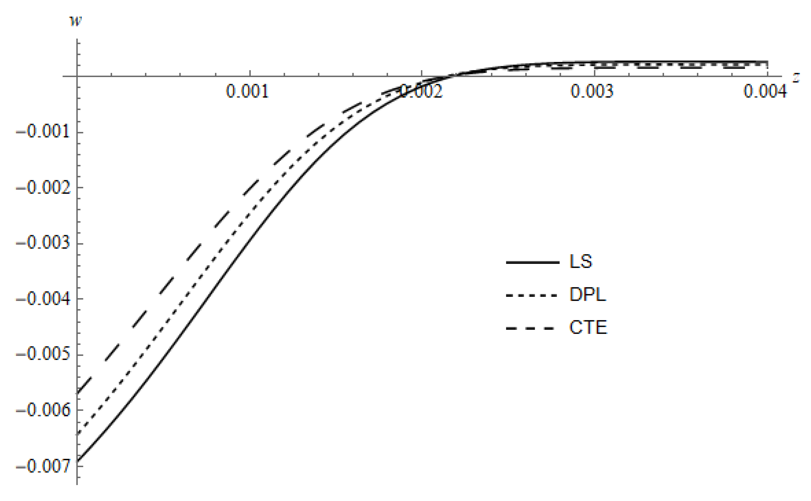
Figure 10 represents the spatial distribution of w for three different models, namely, LS, DPL and CTE; the curves calculated for $h=0$ and $t=4\times {10}^{-3}$, the curve of the DPL model calculated for the value ${\tau }_1=30\times {10}^{-5}$. The figure shows that the value at the irradiated surface is greater for LS and DPL models than the CTE model while the penetration does not affect; this behavior can be interpreted from Figure 5 where the gradient of the temperature of LS and DPL models is smaller than the gradient of the CTE. According to [30], the curves of the CTE and LS for the surface absorption are greater than the case of the volumetric absorption, while the penetration is approximately equal.

Figure 11 represents w for three different models, namely LS, DPL and CTE, the curves calculated for $h\ne 0$ and $t=4\times {10}^{-3}$, the curve of the DPL model calculated for the value ${\tau }_1=30\times {10}^{-5}$. The figure shows that due to cooling, the displacement of the three theories are practically the same. Furthermore, the penetration into the medium is slightly greater in the case of $h\ne 0$ than that of $h=0$ in Figure 10. In the case of cooling, the case of surface absorption shows smaller magnitude and penetration than the case of volumetric absorption [30].

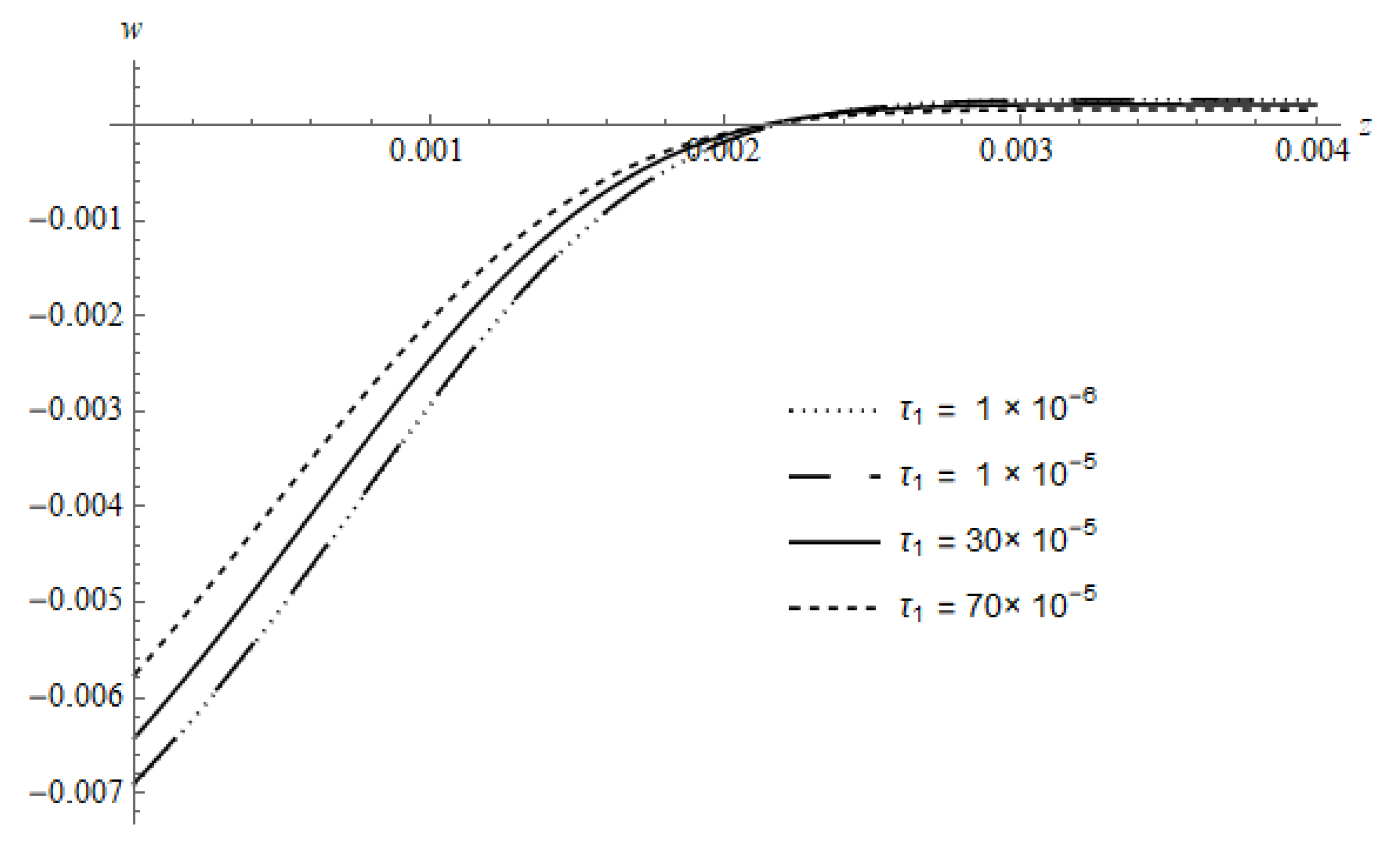
Figure 12 represents the spatial distribution of w of the DPL model calculated for different values of ${\tau }_1$ at a fixed value of ${\tau }_2$ at the time $t=4\times {10}^{-3}$ with $h=0$. It is noted from the figure that the displacement is increased with decreasing ${\tau }_1$, while the penetration is not affected.

Figure 13 represents w of the DPL model calculated for different values of ${\tau }_1$ at a fixed value of ${\tau }_2$ at the time $t=4\times {10}^{-3}$ with $h\ne 0$, from the figure, a very weak effect for ${\tau }_1$ with the existence of cooling being observed, where the curves seem to coincide.

Figure 14 represents the spatial distribution of ${\sigma }_{zz}$ of the DPL model calculated for $h=0$ and ${\tau }_1=30\times {10}^{-5}$ at several times, beside a small figure representing ${\sigma }_{zz}$ near the irradiated surface. According to Equation (13), the behavior of ${\sigma }_{zz}$ is due to the effect of the gradient of the displacement and the temperature. The gradient of the displacement is practically has its effect in a region very close to the irradiated surface and its effect increases with time (see Figure 9). As z increases, the effect of the gradient of w vanishes and then the effect of the temperature appears evidently as in Figure 4. For the times ($t=3\times {10}^{-3}$, $t=3.4\times {10}^{-3}$) or before the temperature reaches its maximum, the stress does not possess a positive peak in the vicinity of the irradiated surface, the positive peak appears for ($t=4\times {10}^{-3}$, $t=5\times {10}^{-3}$).

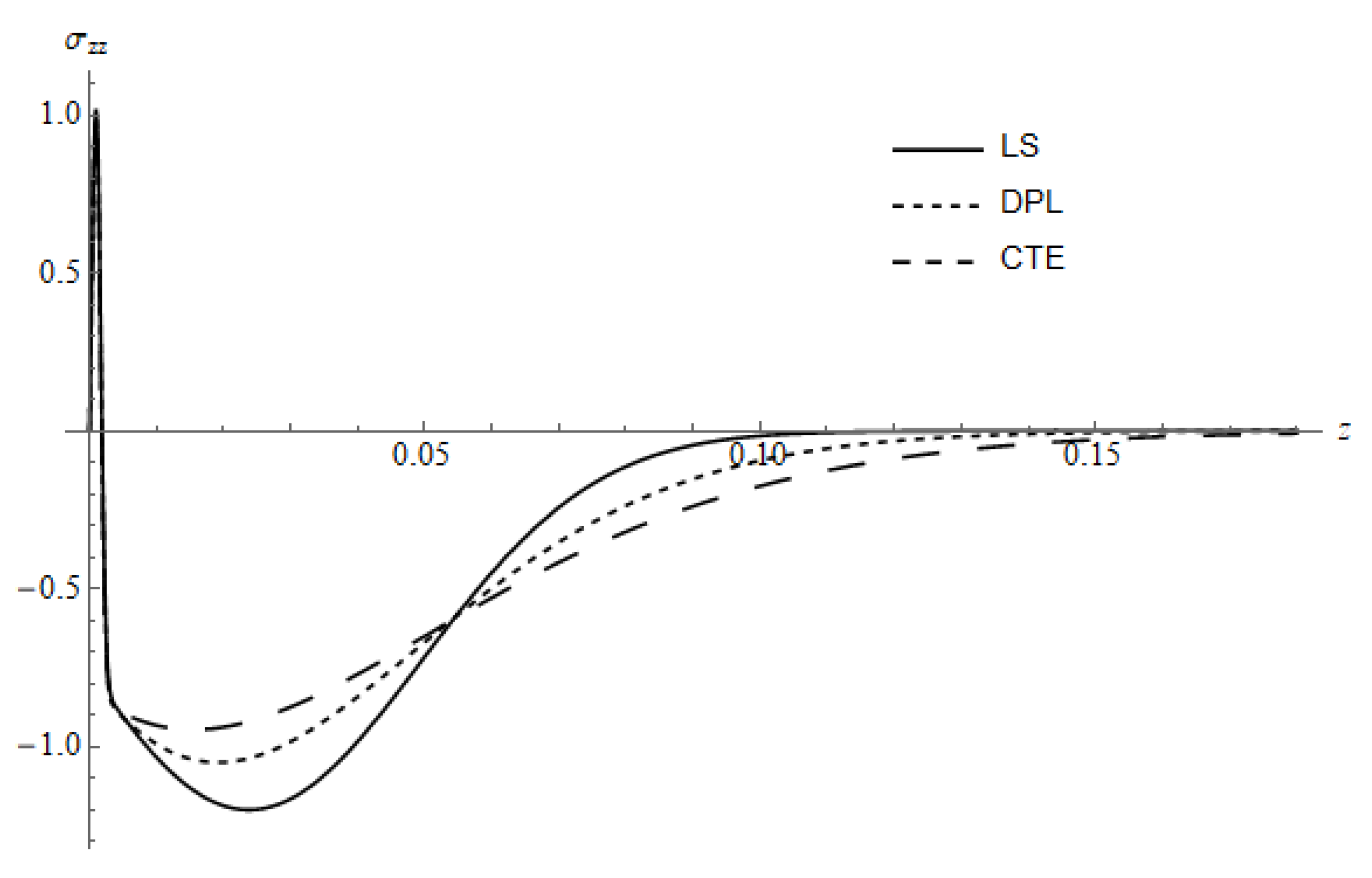
Figure 15 represents ${\sigma }_{zz}$ for three different models, namely LS, DPL and CTE, calculated for $h=0$ and time $t=4\times {10}^{-3}$, the curve of the DPL model calculated for the value ${\tau }_1=30\times {10}^{-5}$. In the vicinity of the irradiated surface, the positive peak of ${\sigma }_{zz}$ is greater for the generalized theories (LS, DPL) than the CTE model. By increasing the z-value, the temperature effect becomes pronounced and shows the same behavior as in Figure 5. According to [30], both positive and negative peaks of the stress ${\sigma }_{zz}$ are greater in the case of surface absorption than the case of the volumetric absorption for LS and CTE models.

Figure 16 represents ${\sigma }_{zz}$ for three different models, namely LS, DPL and CTE, calculated for $h\ne 0$ and time $t=4\times {10}^{-3}$, the curve of the DPL model calculated for the value ${\tau }_1=30\times {10}^{-5}$. This figure agrees with Figure 6 and Figure 11,where in a region closest to the irradiated surface, the cooling has a slight effect on displacement and so its gradient. By increasing the z-value, the behavior of the temperature appears with the cooling effect. The figure agrees with the previous one in terms of the effect of the technique of absorption [30].

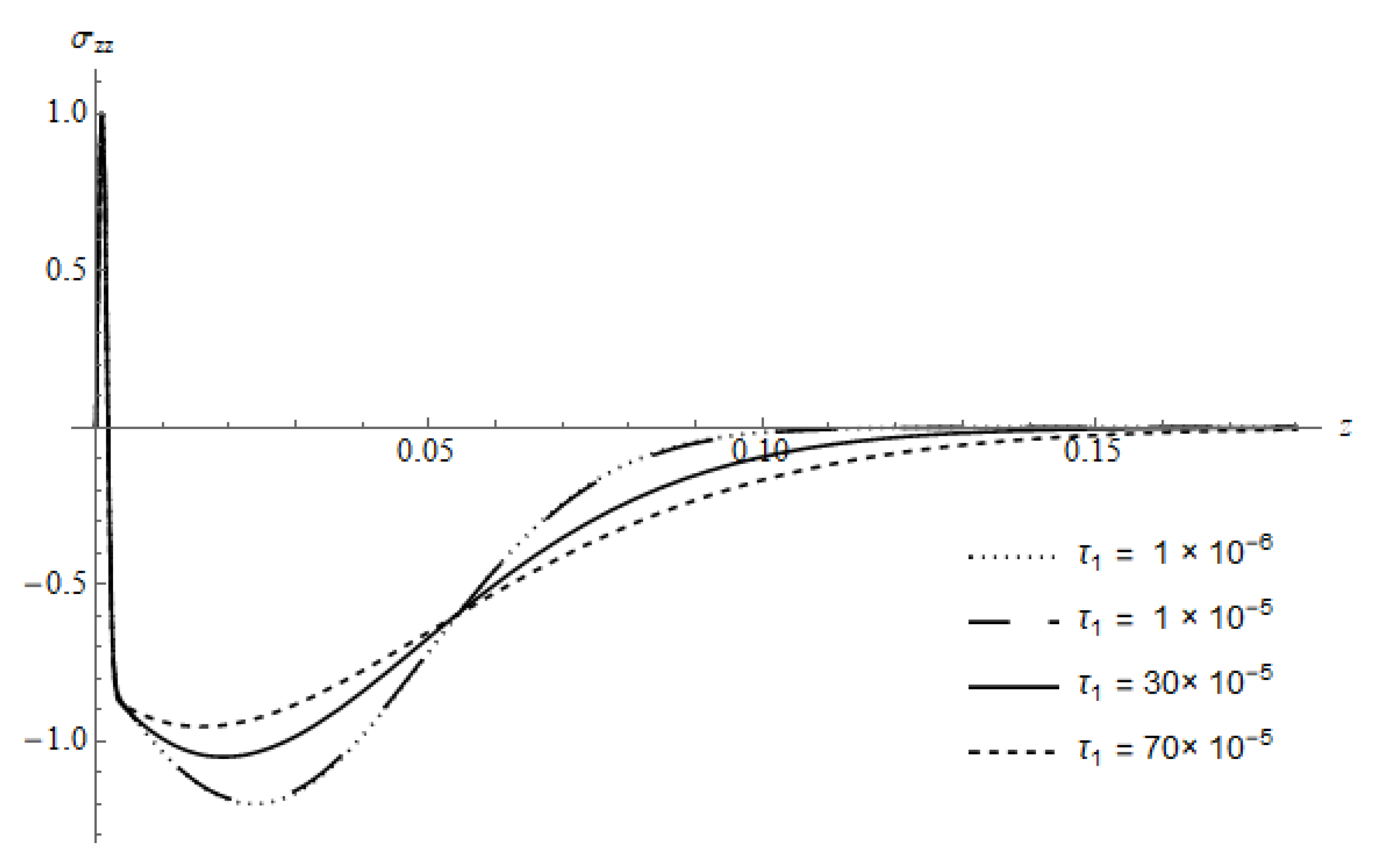
Figure 17 represents the spatial distribution of ${\sigma }_{zz}$ of the DPL model calculated for different values of ${\tau }_1$ at a fixed value of ${\tau }_2$ at the time $t=4\times {10}^{-3}$ with $h=0$. Close to the irradiated surface, the positive peak increases with a decreasing value of ${\tau }_1$. By increasing the z-value ${\sigma }_{zz}$ shows the same behavior of the temperature for the same case (Figure 7).

Figure 18 represents ${\sigma }_{zz}$ of the DPL model calculated for different values of ${\tau }_1$ at a fixed value of ${\tau }_2$ at time $t=4\times {10}^{-3}$ with $h\ne 0$. In the vicinity of the irradiated surface, the stresses seem to coincide with each other, which is due to the cooling effect. By increasing the z-value, the behavior of the temperature with cooling appears evidently.

7. Conclusions

This paper was devoted to study the thermoelastic response induced by volumetric absorption of a uniform laser radiation in a homogeneous and isotropic thermoelastic half-space whose surface is exposed to heat losses. From the above, it can be concluded that:

• The responses induced by the surface absorption are greater than the responses induced by the volumetric absorption, which loses some energy in absorbing the radiation throughout the medium.
• The results obtained by employing the generalized theories are not in contradiction with the well-known physical phenomena, while the results obtained from the CTE model display its nature evidently.
• In both surface and volumetric absorption, the cooling parameter shows a very slight effect on the displacement and its gradient, while it shows a pronounced effect on the temperature, and it can control the influence of the laser power.
• The response of the DPL model appears as if it were a case between the LS and the CTE models.
• A clear effect is seen on all studied fields for the phase lag of the temperature gradient at a specified value of the phase lag of the heat flux.

References

1. Biot, M.A. Thermoelasticity and irreversible thermodynamics. J. Appl. Phys. 1956, 27, 240–253. [Google Scholar] [CrossRef]
2. Hetnarski, R.B. Coupled one-dimensional thermal shock problem for small times. Arch. Mech. Stosow. 1961, 13, 295–306. [Google Scholar]
3. Hetnarski, R.B. Solution of the coupled problem of thermoelasticityi in the form of series of functions. Arch. Mech. Stosow. 1964, 16, 919–941. [Google Scholar]
4. Boley, B.A.; Tolins, I.S. Transient coupled thermoelastic boundary value problems in half-space. J. Appl. Mech. 1962, 29, 637–646. [Google Scholar] [CrossRef]
5. Lord, H.W.; Shulman, Y. A generalized dynamical theory of thermoelasticity. J. Mech. Phys. Solids 1967, 15, 299–309. [Google Scholar] [CrossRef]
6. Ignaczak, J. A uniqueness theorem for stress-temperature equations of dynamic thermoelasticity. J. Therm. Stresses 1978, 1, 163–170. [Google Scholar] [CrossRef]
7. Ignaczak, J. A note on uniqueness in thermoelasticity with one relaxation time. J. Therm. Stresses 1982, 5, 257–263. [Google Scholar] [CrossRef]
8. Sherief, H.; Dhaliwal, R. Generalized one-dimensional thermal shock problem for small times. J. Therm. Stresses 1981, 4, 407–420. [Google Scholar] [CrossRef]
9. Sherif, H. Fundamental solution of the generalized themoelastic problem for short times. J. Therm. Stresses 1986, 9, 151–164. [Google Scholar] [CrossRef]
10. Sherief, H.; Hamza, F. Generalized thermoelastic problem of a thick plate under axisymmetric temperature distribution. J. Therm. Stresses 1994, 17, 435–452. [Google Scholar] [CrossRef]
11. Green, A.E.; Lindsay, K.A. Thermoelasticity. J. Elast. 1972, 2, 1–7. [Google Scholar] [CrossRef]
12. Green, A.E.; Naghdi, P.M. Thermoelasticity without energy dissipation. J. Elast. 1993, 31, 189–208. [Google Scholar] [CrossRef]
13. Hetnarski, R.B.; Ignaczak, J. Soliton-like waves in a low temperature nonlinear thermoelastic solid. Int. J. Eng. Sci. 1996, 34, 1767–1787. [Google Scholar] [CrossRef]
14. Ozisik, M.N.; Tzou, D.Y. On the wave theory of heat conduction. J. Heat Transf. (ASME) 1994, 116, 526–535. [Google Scholar] [CrossRef]
15. Tzou, D.Y. A unified field approach for heat conduction from macro-to micro-scales. J. Heat Transf. 1995, 117, 8–16. [Google Scholar] [CrossRef]
16. Tzou, D.Y. Experimental support for the lagging behavior in heat propagation. J. Thermophys. Heat Transfer 1995, 9, 686–693. [Google Scholar] [CrossRef]
17. RoyChoudhuri, S.K.R. One-dimensional thermoelastic waves in elastic half-space with dual phase-lag effects. J. Mech. Mater. Struct. 2007, 2, 489–503. [Google Scholar] [CrossRef] [Green Version]
18. Abouelregal, A. A problem of a semi-infinite medium subjected to exponential heating using a dual-phase-lag thermoelastic model. Appl. Math. 2011, 2, 619–624. [Google Scholar] [CrossRef] [Green Version]
19. El-Karamany, A.S.; Ezzat, M.A. On the Dual-Phase-Lag thermoelasticity theory. Meccanica 2014, 49, 79–89. [Google Scholar] [CrossRef]
20. Abbas, I.; Zenkour, A.M. Dual-Phase-Lag model on thermoelastic interactions in a semi-infinite medium subjected to ramp-type heating. J. Comput. Theor. Nanos. 2014, 11, 642–645. [Google Scholar] [CrossRef]
21. Marin, M.; Broadbridge, P.; Öchsner, A. Well-posed dual-phase-lag model of a thermoelastic dipolar body. ZAMM Z. Angew. Math. Mech. 2017, 97, 1645–1658. [Google Scholar] [CrossRef]
22. Hassan, A.F.; El-Nicklawy, M.M.; EL-Adwi, M.K.; Nasr, E.M.; Hemida, A.A.; El-Ghaffar, O.A.A. Heating effects induced by a pulsed laser in a semi-ifinite target in view of the theory of linear systems. Opt. Laser Technol. 1996, 28, 337–343. [Google Scholar] [CrossRef]
23. McDonald, F.A. On the precursor in laser-generated ultrasound waveforms in metals. Appl. Phys. Lett. 1990, 56, 230–232. [Google Scholar] [CrossRef]
24. Dubois, M.; Enguehard, F.; Bertrand, L. Modeling of laser thermoelastic generation of ultrasound in an orthotrobic medium. Appl. Phys. Lett. 1994, 64, 554–556. [Google Scholar] [CrossRef]
25. Wang, X.; Xu, X. Thermoelastic wave induced by pulsed laser heating. Appl. Phys. A 2001, 73, 107–114. [Google Scholar] [CrossRef]
26. Henain, E.F.; Hassan, A.F.; Megahed, F.; Tayel, I.M. Thermo-elastic half space under illumination of a laser beam by using Lord and Shulman theory. J. Therm. Stresses 2014, 37, 51–72. [Google Scholar] [CrossRef]
27. Yossef, H.M.; El-Bary, A.A. Thermoelastic material response due to laser pulse heating in context of four theorems of thermoelasticity. J. Therm. Stresses 2014, 37, 1379–1389. [Google Scholar] [CrossRef]
28. Allam, M.N.M.; Tayel, I.M. Generalized thermoelastic functionally graded half space under surface absorption of laser radiation. J. Theor. Appl. Mech. 2017, 55, 155–165. [Google Scholar] [CrossRef]
29. Abbas, I.A.; Marin, M. Analytical solution of thermoelastic interaction in a half-space by pulsed laser heating. Phys. E Low-Dimens. Syst. Nanostruct. 2017, 87, 254–260. [Google Scholar] [CrossRef]
30. Tayel, I.M.; Hassan, A.F. Heating a thermoelastic half space with surface absorption pulsed laser using fractional order theory of thermoelasticity. J. Theor. Appl. Mech. 2019, 57, 489–500. [Google Scholar] [CrossRef]
31. Debnath, L.; Bhatta, D. Integral Transforms and Their Applications; Taylor and Francis: New York, NY, USA, 2015. [Google Scholar]
Figure 1. The irradiating laser pulse profile g ( t ) and the time dependence of the surface temperature θ ( 0 , t ) calculated for three different theories for h = 0 .
Coatings 10 00228 g001
Figure 2. The irradiating laser pulse profile g ( t ) and the time dependence of the surface temperature θ ( 0 , t ) calculated for three different theories for h 0 .
Coatings 10 00228 g002
Figure 3. The irradiating laser pulse profile g ( t ) and the time dependence of the surface temperature θ ( 0 , t ) of the DPL theory calculated for h = 0 and different values of τ 1 .
Coatings 10 00228 g003
Figure 4. The temperature θ ( z , t ) of the DPL theory as a function of z calculated for h = 0 at different times.
Coatings 10 00228 g004
Figure 5. The temperature θ ( z , t ) of three theories as a function of z calculated for h = 0 at t = 4 × 10 3 .
Coatings 10 00228 g005
Figure 6. The temperature θ ( z , t ) of three theories as a function of z calculated for h 0 at t = 4 × 10 3 .
Coatings 10 00228 g006
Figure 7. The temperature θ ( z , t ) of the DPL theory as a function of z calculated for h = 0 and different values of τ 1 at t = 4 × 10 3 .
Coatings 10 00228 g007
Figure 8. The temperature θ ( z , t ) of the DPL theory as a function of z calculated for h 0 and different values of τ 1 at t = 4 × 10 3 .
Coatings 10 00228 g008
Figure 9. The displacement w ( z , t ) of the DPL theory as a function of z calculated for h = 0 at different times.
Coatings 10 00228 g009
Figure 10. The displacement w ( z , t ) of three theories as a function of z calculated for h = 0 at t = 4 × 10 3 .
Coatings 10 00228 g010
Figure 11. The displacement w ( z , t ) of three theories as a function of z calculated for h 0 at t = 4 × 10 3 .
Coatings 10 00228 g011
Figure 12. The displacement w ( z , t ) of the DPL theory as a function of z calculated h = 0 and different values of τ 1 at t = 4 × 10 3 .
Coatings 10 00228 g012
Figure 13. The displacement w ( z , t ) of the DPL theory as a function of z calculated h 0 and different values of τ 1 at t = 4 × 10 3 .
Coatings 10 00228 g013
Figure 14. The stress σ z z ( z , t ) of the DPL theory as a function of z calculated for h = 0 at different times.
Coatings 10 00228 g014
Figure 15. The stress σ z z ( z , t ) of three theories as a function of z calculated for h = 0 at t = 4 × 10 3 .
Coatings 10 00228 g015
Figure 16. The stress σ z z ( z , t ) of three theories as a function of z calculated for h 0 at t = 4 × 10 3 .
Coatings 10 00228 g016
Figure 17. The stress σ z z ( z , t ) of the DPL theory as a function of z calculated h = 0 and different values of τ 1 at t = 4 × 10 3 .
Coatings 10 00228 g017
Figure 18. The stress σ z z ( z , t ) of the DPL theory as a function of z calculated h 0 and different values of τ 1 at t = 4 × 10 3 .
Coatings 10 00228 g018