Article

Modeling and Optimization Approaches of Laser-Based Powder-Bed Fusion Process for Ti-6Al-4V Alloy

by
Behzad Fotovvati
1,
Madhusudhanan Balasubramanian
2 and
Ebrahim Asadi
1,*
1
Department of Mechanical Engineering, The University of Memphis, Memphis, TN 38152, USA
2
Department of Electrical and Computer Engineering, The University of Memphis, Memphis, TN 38152, USA
*
Author to whom correspondence should be addressed.
Coatings 2020, 10(11), 1104; https://doi.org/10.3390/coatings10111104
Submission received: 26 October 2020 / Revised: 10 November 2020 / Accepted: 13 November 2020 / Published: 18 November 2020
(This article belongs to the Special Issue Novel Materials and Processes for Metal Additive Manufacturing)

Abstract

:
Laser-based powder-bed fusion (L-PBF) is a widely used additive manufacturing technology that contains several variables (processing parameters), which makes it challenging to correlate them with the desired properties (responses) when optimizing the responses. In this study, the influence of the five most influential L-PBF processing parameters of Ti-6Al-4V alloy—laser power, scanning speed, hatch spacing, layer thickness, and stripe width—on the relative density, microhardness, and various line and surface roughness parameters for the top, upskin, and downskin surfaces are thoroughly investigated. Two design of experiment (DoE) methods, including Taguchi L25 orthogonal arrays and fractional factorial DoE for the response surface method (RSM), are employed to account for the five L-PBF processing parameters at five levels each. The significance and contribution of the individual processing parameters on each response are analyzed using the Taguchi method. Then, the simultaneous contribution of two processing parameters on various responses is presented using RSM quadratic modeling. A multi-objective RSM model is developed to optimize the L-PBF processing parameters considering all the responses with equal weights. Furthermore, an artificial neural network (ANN) model is designed and trained based on the samples used for the Taguchi method and validated based on the samples used for the RSM. The Taguchi, RSM, and ANN models are used to predict the responses of unseen data. The results show that with the same amount of available experimental data, the proposed ANN model can most accurately predict the response of various properties of L-PBF components.

1. Introduction

Laser-based powder-bed fusion (L-PBF) is a widely adopted additive manufacturing (AM) methodology used to manufacture high-performance metallic parts with complex geometries via selective laser scanning of thin layers of metal powders. Numerous studies have investigated the correlations between the L-PBF processing parameters and various properties of the fabricated parts, such as surface quality, internal porosity, and mechanical performance [1,2,3,4]. Chen [5] categorized AM modeling studies into empirical, analytical, and numerical models, along with machine learning techniques. A full factorial design of experiment (DoE) consists of an equal number of replicates of all the possible combinations of the levels (values) of each of the factors (processing parameters). For instance, for five factors each with five levels, 55 or 3125 experiments are required for this method. The advantage of this approach is having the exact response for the effects of parameters and all of the combinations of their interactions [6]. However, conducting a full factorial DoE to determine L-PBF process parameters for novel materials is practically impossible. The reason is the high costs and time associated with manufacturing and characterizing these samples and modeling the correlations between the characterization and the process parameters. Therefore, fractional factorial DoE methods are required to evaluate the most significant process variables and to optimize the performance of the products.
The Taguchi method with orthogonal arrays is a fractional factorial DoE method that is a simple and powerful tool. It provides a systematic approach to optimize designs for quality and cost [7]. The Taguchi method has been employed to optimize the settings of process parameters in metal AM processes such as directed energy deposition (DED) [8,9,10] and fused deposition modeling (FDM) [11,12]. Liu et al. [8] optimized the DED process parameters, including laser power, scanning speed, powder feeding rate, and shielding gas flow rate, to obtain the highest density of AlSi10 Mg parts using the Taguchi L25 orthogonal array. Manjunath et al. [9] employed a Taguchi L9 orthogonal array design to optimize the DED process of colmonoy 52 SA, which is a hard nickel-chromium-boron alloy. They obtained the best interfacial bonding between the substrate and the deposition material by measuring the hardness variations in these regions. Yang et al. [10] pointed out the limitation of the Taguchi method in optimizing only a single performance characteristic at a time in the DED processing of Inconel 625. Donstov et al. [12] found the application of this method useful in improving the physical, mechanical, and tribological properties of FDM-manufactured metal-polymer composite samples in terms of uniformity of powder mixing as well as the structural uniformity of the produced samples. The Taguchi method has also been used for the L-PBF process optimization for various materials, including SS316 L [13,14], AlSi10 Mg [15,16], CoCrMo [17], Inconel [18], and Titanium alloys [17,19]. Joguet et al. [17] used this method to evaluate the effects of four L-PBF processing parameters, including laser spot size, hatch spacing, exposure time, and laser focal point distance, on porosity content of CoCrMo and Ti40 parts. Using the Taguchi approach, Kuo and Yang [20] obtained optimal laser power, scanning speed, hatch spacing, and layer thickness for fabricating plastic injection molds with higher hardness and better gas permeability. They reported the layer thickness as the most significant parameter affecting the response properties. Rathod and Karia [16] reported a similar conclusion for the significance of the layer thickness in determining the hardness and surface roughness. Sathish et al. [18] employed the Taguchi method to examine the influence of build orientation and heat treatment on the coefficient of friction in Inconel 718 samples fabricated by L-PBF. Jiang et al. [13] examined the effects of three factors—laser power, scanning speed, and hatch spacing—at three levels on three properties of L-PBF parts: top surface roughness, hardness, and density. They reported laser power as the most important parameter affecting all the examined properties. Calignano et al. [15] found that the scanning speed had the biggest impact on the surface roughness of the components fabricated by the L-PBF process. Although the reason for this difference in conclusions is unclear, it may be attributed to differences in the materials (stainless steel vs. aluminum alloys) or differences in the machines (EP250 vs. EOSINT M270) used for these experiments.
The response surface method (RSM) is another DoE method to characterize design parameter settings to enhance system performance or output. The RSM uses a combination of the DoE, regression analysis, and optimization techniques to optimize a stochastic response value. The RSM can be used with a full factorial DoE or fractional factorial DoE. However, a full factorial DoE with many factors requires a very large number of observations, as previously explained. Therefore, reducing the size of a full factorial experiment can be very helpful when more than three factors contribute to a response in an experiment. This is where the fractional factorial design is useful. In this method, known design properties are used to selectively reduce the size of an experiment [21]. Dada et al. [22] employed a full factorial design along with the RSM as an optimization tool for the laser processing of additively manufactured high entropy alloys. They considered microhardness values of the produced samples as the output response by the variation of laser power and scanning speed. Pant et al. [23] implemented the central composite design in RSM to model and optimize the DED processing of 316 L stainless steel. They considered laser power, scanning speed, and powder flow rate as input parameters, and capture efficiency and clad layer height as the response parameters. Read et al. [24] employed the RSM to evaluate the best settings of laser power, scanning speed, hatch spacing, and scanning island size to optimize the porosity level of L-PBF-manufactured AlSi10 Mg parts. They found the critical energy density point that provided the minimum pore fraction for this alloy to be 60 J/m3. El-Sayed et al. [25] used the RSM to propose the optimum process parameters, including laser power, scanning speed, and hatch spacing, for Ti-6Al-4V medical implant applications and concluded that higher energy densities resulted in lower surface roughness and lower porosity levels. Gajera et al. [26] used the Box-Behnken design of the RSM and established a relationship between the L-PBF process parameters and surface roughness values of CL50 WS steel parts to compare two optimization algorithms: a genetic algorithm and the Jaya algorithm. Bartolomeu et al. [27] manufactured Ti-6Al-4V samples by varying three processing parameters (i.e., laser power, scanning speed, and hatch spacing) at three levels in the L-PBF process and used the RSM to analyze the experimental results of shear stress, hardness, and density. They obtained a quadratic model for each of the output properties and presented a response surface for them. They achieved relatively good adequacy for their models with a coefficient of determination R2 of 0.62–0.68. Please note that R2 has values between 0–1 (higher values show higher accuracies) and increases when other higher-order terms are added to the model. Hence, an adjusted R2 is recommended as a criterion for the model adequacy. The adjusted R2 for their models ranged from 0.55–0.61. Krishnan et al. [28] used a full factorial DoE on three levels of three factors—laser power, scanning speed, and hatch spacing—to evaluate the most significant factor affecting the mechanical properties of L-PBF-manufactured AlSi10 Mg samples. They concluded that hatch spacing was the parameter with the most significant influence. Using the same approach, Pawlak et al. [29] fabricated AZ31 magnesium parts with relative densities higher than 99.5% using the L-PBF process. Sharma et al. [30] used the Taguchi method and RSM to investigate the influence of the laser power, scanning speed, and hatch spacing on density and surface roughness of PBF-fabricated AlSi10 Mg samples and reported the hatch spacing as the most significant factor in determining the output responses. Wang et al. [31] combined the two methods, i.e., Taguchi and RSM, to study the effect of the laser power, scanning speed, and hatch spacing, on the mechanical properties and microstructure of nickel-based superalloy samples fabricated by the PBF process. They applied linear, two-factor-interaction, and quadradic models to obtain response surfaces for the tensile strength of the manufactured samples and observed the quadratic modeling of this response yields to the lowest error value among all the tested models.
Machine learning (ML) techniques can carry out complex pattern recognition and regression analysis without constructing and solving the underlying physical models. This method is widely used in modeling, prediction, and analyzing the interaction of parameters in different industries, such as manufacturing, aerospace, and biomedicine [32,33]. Among ML algorithms, artificial neural networks (ANNs), which are mathematical models mapping an input space to an output space, are the most extensively used techniques because of their strong computational power and sophisticated architectures [34]. The architecture of an ANN consists of an input layer, one or more hidden layers, and an output layer [35]. One of the most widely used training methods is back-propagation, in which gradients are computed iteratively for each layer using the mathematical chain rule [36]. Once the ANN is trained, it can predict the responses based on unseen input values. Some of the applications of ML and ANNs to AM have focused on real-time process monitoring. Zhang et al. [37] employed a conventional neural network (CNN) for quality level identification in the L-PBF process through in situ monitoring of laser melt-pool. Paul et al. [38] used an ML technique (decision tree) for computational process modeling of the direct metal deposition process to obtain a predictive tool for temperature profiles in this process. Caggiano et al. [39] developed a deep CNN for in situ material defect-recognition in the L-PBF process. Shevchik et al. [40] combined acoustic emission sensors with ML for in situ quality monitoring in the L-PBF process. Many engineering and manufacturing applications have successfully implemented the ANN methodology as a beneficial empirical modeling method in metal and non-metal AM processes [41,42]. Marmarelis and Ghanem [30] performed an ML technique, called diffusion maps, to infer the dependence structure between laser power, scanning speed, and hatch spacing and mechanical properties of L-PBF-manufactured AlSi10 Mg samples. Guo et al. [43] proposed an ML-based classifier to assess whether a metal cellular structure can be successfully manufactured using a given set of L-PBF processing parameters. Their proposed model works based on classification algorithms and it can classify the failures in the process caused by residual stresses, cracking, and delamination. Nguyen et al. [33] presented an optimization tool that worked based on ML to predict the density of Ti-6Al-4V parts manufactured with any variation in the L-PBF process parameters, including laser power (80–180 W), scanning speed (800–2500 mm/s), layer thickness (20–80 µM), and hatch spacing (30–100 µM). Zhang et al. [44] developed a prediction model for the high-cycle fatigue life of L-PBF-manufactured stainless steel parts using ML approaches. Li and Anand [45] trained a feed-forward back-propagation ANN to predict inherent strain obtained by thermo-mechanical simulation for different given hatch patterns that are adopted during the L-PBF process. Bhardwaj and Shukla [33] simulated a single track deposition in DED of Ti-15 Mo alloy and used their simulation results for training a feed-forward back-propagation ANN with seven hidden layers and Levenberg-Marquardt training algorithm. They used three input parameters, i.e., laser power, scanning speed, and powder feed rate, to predict the track dilution as the single response of the network. The mean square of the prediction error percentage was calculated to evaluate the goodness of the fitted model. Yan [46] proposed an optimization algorithm based on a back-propagation ANN to improve the dimensional precision in the FDM process. Marrey et al. [47] proposed a framework to input the laser power and scanning speed to an ANN and predict the microstructure and mechanical properties of PBF-fabricated 316 L stainless steel parts. Tran and Lo [48] performed finite element heat transfer simulations to correlate the L-PBF process parameters, including laser power and scanning speed, to the melt-pool dimensions and peak temperature in the L-PBF processing of 316 L stainless steel. Then, they used the simulated results to train an ANN to predict the melt-pool characteristics based on the input variables. Also, they extended their work [49] to add hatch spacing and scan length to the input parameters of their model. Rahimi et al. [50] used the combination of a central composite design of RSM and a feed-forward back-propagation ANN to investigate the effect of process parameters in the laser engraving process of Al-SiC composites on the depth, width, and contrast of engraved zone. Mehrpouya et al. [51] presented a an ANN-based prediction model for strain recovery ratios in the AM of NiTi shape memory alloys. Khorasani et al. [52] implemented an ANN with three hidden layers with four, three, and two hidden nodes to predict a single response (output) of the top surface roughness of Ti-6 Al-4V parts based on the input parameters of laser power, scanning speed, hatch spacing, scan pattern increment angle, and heat treatment (HT) condition, i.e., different HT temperatures and cooling times. According to their results, the HT condition, which is a post-process parameter, was the dominant factor in determining the top surface roughness of L-PBF-manufactured parts. Furthermore, they concluded that higher energy densities (higher laser power and lower scanning speed) resulted in parts with lower surface quality. Akhil et al. [53] used an ANN with five hidden nodes in one hidden layer to extract image texture parameters from surface images and predict the top surface roughness of L-PBF-manufactured Ti-6Al-4V parts.
All these studies, similar to DoEs based on the Taguchi method and the RSM, are limited to a single target property for optimization based on the variation in a few AM process parameters. Most notably, layer thickness has been precluded from the list of the L-PBF processing parameters for optimization. However, Hiren et al. [54] reported the layer thickness as the most significant parameter in the L-PBF process. Furthermore, there is a lack of comprehensive studies comparing the optimization of L-PBF processing parameters via the Taguchi method, the RSM, and ANNs. In this study, the five most influential parameters, including laser power, scanning speed, hatch spacing, layer thickness, and stripe width, are taken as the design factors for L-PBF processing of Ti-6Al-4V alloy. The top, upskin, and downskin surface roughness, microhardness, and relative density are considered the target properties for the optimization of the L-PBF processing parameters. First, L25 Taguchi orthogonal arrays are used for the DoE of L-PBF process parameters in five levels. Second, a fractional factorial DoE resulting in 1/125th of the full factorial experiments is used for the RSM and ANN optimizations of the processing parameters. Additionally, the correlations between the L-PBF process parameters and the target properties are modeled and extensively discussed. Finally, the sets of optimum processing parameters predicted by each method are determined and compared.

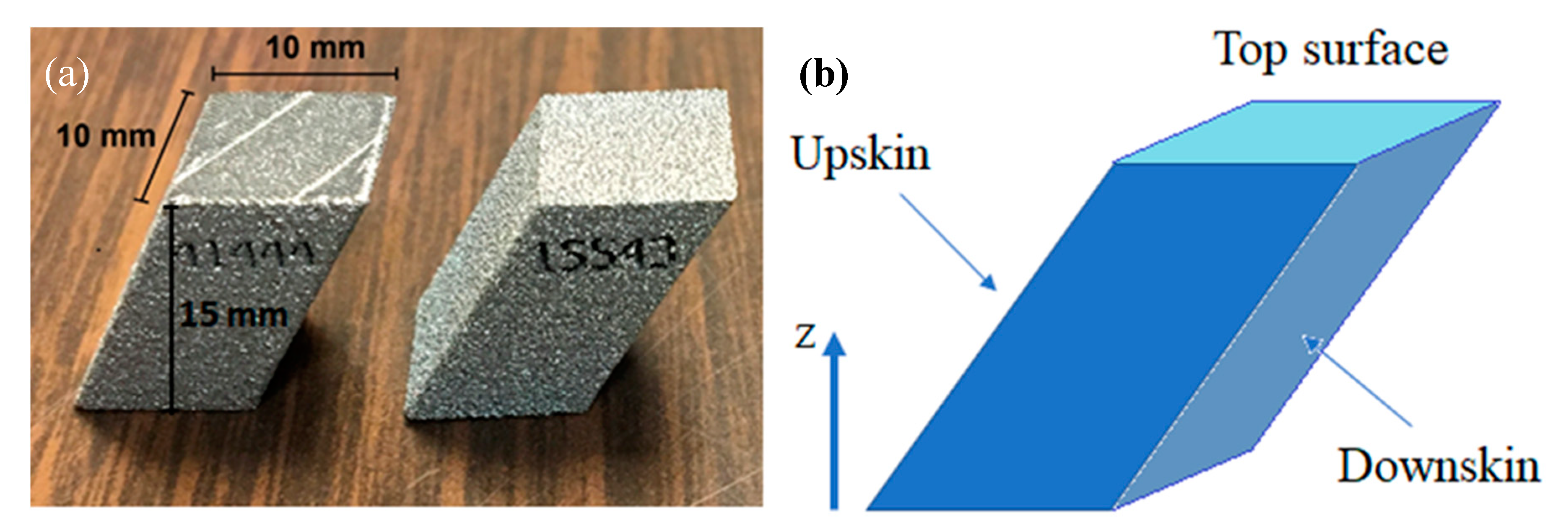
2. Materials and Methods

All L-PBF of the Ti-6Al-4V samples and powder characterization were performed in the University of Memphis Metal Additive Manufacturing Laboratory with a temperature of 23 ± 3 °C and humidity of 30% ± 5%. In our previous studies [55,56] we reported the physical and chemical characterization of the used powders. An EOS M290 machine (EOS GmbH Electro Optical Systems, Krailling, Germany) was used to perform the L-PBF of the Ti-6Al-4V parts. The samples were manufactured when the equipment was only one year old. Therefore, the laser performance is reliable. All the samples were manufactured in five consecutive runs (with five different values for the layer thickness). Therefore, the laser life is very unlikely to be affected from the beginning to the end of the experimentation. The stripe scanning strategy with zero stripe gap and a scan pattern increment angle of 67° was used for manufacturing all the samples. The laser power (p), scanning speed (v), hatch spacing (h), layer thickness (t), and stripe width (s) are the L-PBF parameters, and the effects of these parameters on the surface roughness, density, and microhardness of the manufactured samples were studied in this research.
Figure 1 illustrates the nominal geometry of the samples and two examples of the samples fabricated using the L-PBF process. The samples were rectangular cuboids with a 60° overhang that enabled analysis of the influence of process parameters on the characteristics of the upskin and downskin surfaces in addition to the top surface of the samples. Overall, the following seven roughness parameters—three surface roughness and four line roughness parameters—were measured: top, upskin, and downskin surface roughness and upskin/downskin horizontal/vertical line roughness. The horizontal lines were perpendicular to the z-axis, whereas the vertical lines were oriented in the z-direction. These roughness parameters were measured using a Keyence model VHX-6000 digital microscope (Keyence, Osaka, Japan) following ASME B46.1.
For microhardness testing, the samples were mounted and polished in three levels, i.e., plane grinding to reach a cross-section surface at the center of the sample, fine grinding, and polishing to obtain a mirror finish. A Shimadzu HMV-G microhardness tester (Shimadzu, Kyoto, Japan) with a Vickers indenter was used to perform the tests in rectangular patterns of indentations (3 by 5 points) on each sample. The mean value of these 15 indentations was calculated and considered to be the representing value of the microhardness of each sample. The relative density measurements of the samples were conducted using the Archimedes method following ASTM B311—17 [57].

3. DoE for the L-PBF Process Parameters

The first step in DoE methodologies is to determine the parameters and their levels to be tested. The process parameters and corresponding levels considered for this research are shown in Table 1. The ranges for the process parameters were chosen considering the manufacturability of parts using various combinations of the parameters. The criterion used to evaluate the part manufacturability was the energy density absorbed by the material during the L-PBF process, which can be estimated by E = p/(v·h·t). Too high and too low energy densities result in failure in the manufacturing of the samples. One should note that these ranges may be different when using different manufacturing systems. The recommended values by the equipment manufacturers are within the chosen ranges. If the optimal points fall in the frontiers of the experiment, new DoE should be carried out where the number of factors is reduced to the ones, whose optimum values fall on the range limits, with a new range around their potential optimum value. The experimental design calculations and analysis of this study were carried out using Minitab 18.1 (Minitab Inc., State College, PA, USA).

3.1. Taguchi Method

To obtain the parameter combinations for the experiments of the Taguchi method, orthogonal arrays were used, which can be obtained from any available Taguchi reference manual. For five factors, which have five levels each, the L25 Taguchi orthogonal arrays are used in this study and listed in Table A1 in the Appendix A. The next step was to calculate the signal-to-noise (S/N) ratio. In every DoE, a higher value of the signal and lower value of noise are desired (regardless of the property), so the best design has the largest S/N ratio. The S/N ratio η is defined as follows:
η = 10 × l o g 10 ( M S D )
where MSD is the mean square deviation of the output characteristics and its formulation is determined based on the research objective, which can be minimizing, maximizing, or reducing the discrepancies between the predicted response and the target value. The corresponding MSD formulas are as follows:
MSD = 1 n i = 1 n y i 2
for minimization,
MSD = 1 n i = 1 n 1 y i 2
for maximization, and
MSD = 1 n i = 1 n ( y i m ) 2
for decreased variation, where yi is the ith observed response value, n is the number of test results, and m is the target value of the response.

3.2. Response Surface Method

A fractional factorial design was employed in this study to design the process parameter combinations for the RSM. In general, in an experiment with k factors, each of which has l levels, an lk-p design is a fractional factorial design in lk−p runs. As this study has five factors in five levels, a 55−3 design was chosen, which requires 52 or 25 runs, which is only 1/125th of the full factorial design observations (55 runs). To generate 25 runs for a 55−3 design, the 25 combinations of a 52 full factorial design were placed in the first two columns of the table. The cells of the three remaining columns were generated using the cells in the first two columns according to the following equations [58]:
x 3 = x 1 + x 2 ,   x 4 = x 1 + 2 x 2 ,   x 5 = x 1 + 3 x 2
where xi is the ith column of the table. Mod 5 indicates that the modulus of the operation was 5, which was employed in the construction of five-level designs (under these conditions, any multiple of 5 equals zero). The fractional factorial design combinations of the factor levels for the number of experiments are shown in Table A2 in the appendix.
The objective of the RSM is to formulate the response as a function of contributing factors and to find the best set of factor levels, which provides the optimum response value based on the research goals. Quadratic relationships are of more interest to researchers because of two main reasons: first, linear models are not capable of capturing any two-parameter influence on the response, and second, cubic and higher degree interactions add to the cost of experiments and complexity in determining the RSM functions. In the present study, the results obtained by the Taguchi method indicated that the stripe width had a negligible effect on the measured responses; therefore, this factor was excluded from the rest of the study, i.e., the RSM and ANN. A quadratic behavior of the response of a system of four factors can be modeled as follows:
y = β 0 + β 1 x 1 + β 2 x 2 + β 3 x 3 + β 4 x 4 + β 12 x 1 x 2 + β 13 x 1 x 3 + β 14 x 1 x 4 + β 23 x 2 x 3 + β 24 x 2 x 4 + β 34 x 3 x 4 + β 11 x 1 2 + β 22 x 2 2 + β 33 x 3 2 + β 44 x 4 2
where x 1 through x 4 are the factors and β i are the coefficients to be found using the experimental observations. The response y can be any of the output parameters (e.g., surface roughness, microhardness, etc.) that need to be optimized based on the input processing parameters.

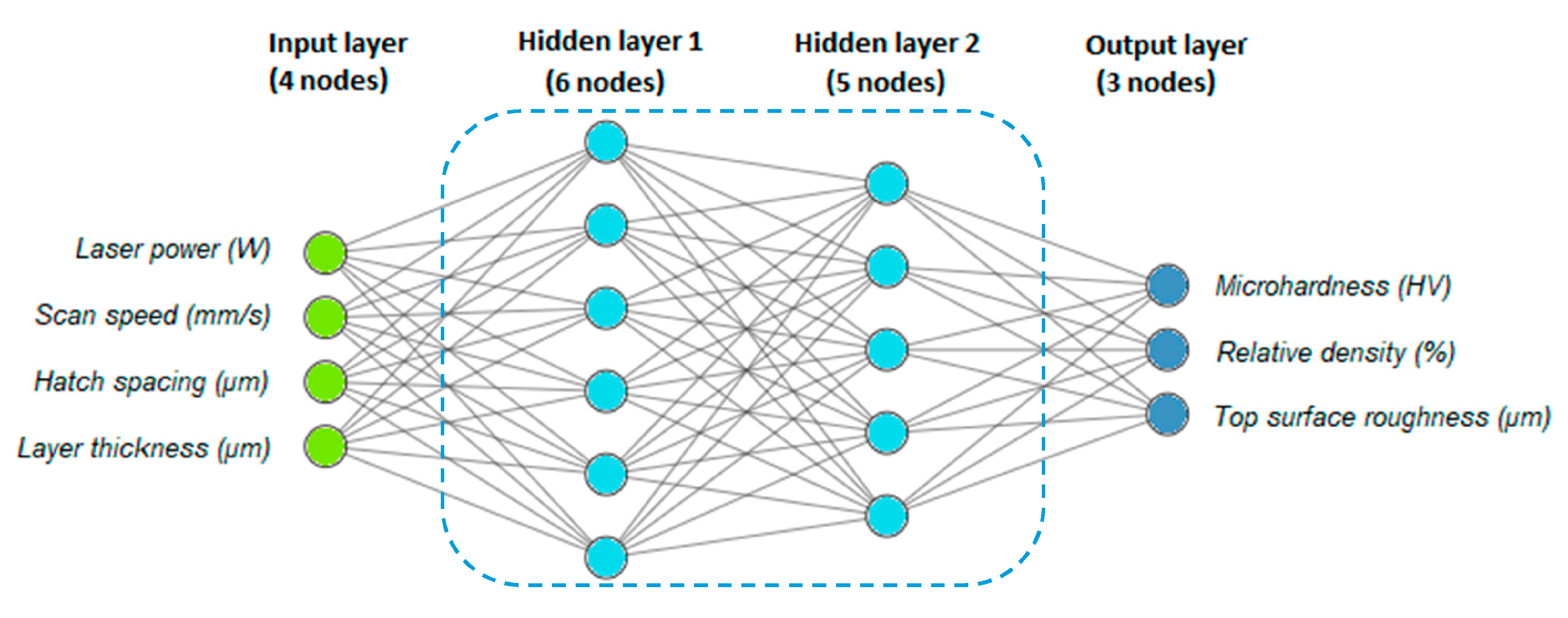
3.3. Artificial Neural Network

Using a trained ANN, all the sample properties can be predicted simultaneously based on the input process parameters. Here, the input layer was designed with four neurons corresponding to the four L-PBF process parameters p, v, t, and h. To reduce the complexity of feed-forward back-propagation ANN, we only considered one of the surface roughness parameters as the network response: top surface roughness. Therefore, the output layer was designed with three neurons to predict microhardness, relative density, and top surface roughness.
The network was trained and tested using raw, unnormalized measures of the input process parameters and output sample properties. A total of 45 samples were used for training and testing the ANN performance. The network was trained using the Bayesian regularization method [59], which, after testing several algorithms, turned out to be the most accurate method for the data used in this study. The Bayesian regularization method does not require a separate group of validation data. Therefore, all available data were divided into a training group and a testing group. To be consistent with the Taguchi method and the RSM and to conduct a fair comparison among them, 25 data samples (55% of all data) were used for training and building the ANN. Therefore, the remaining 20 data samples (45% of all data) that were independent of the training data samples were used for testing the performance of the model.
Figure 2 illustrates the architecture of the feed-forward neural network with two hidden layers implemented in MATLAB (MathWorks, Natick, MA, USA) and used in this study. Qi et al. [34] recommended 5−10 hidden neurons as a starting point for determining the optimal parameters for AM applications. As the number of hidden neurons increases, the training data prediction error decreases, and the network complexity and its capability for capturing more details of data behavior increases. However, with the limited data in this study, increasing the number of hidden neurons makes the network biased to the training data and not capable of predicting new unseen data. After testing several networks with different numbers of hidden layers and different numbers of nodes in each hidden layer, we determined the best performance was exhibited by the model with two hidden layers with six and five neurons in the first and second hidden layers, respectively. Fractional prediction error was used to assess the prediction accuracy and performance of the Taguchi method, the RSM, and the ANN. This parameter is defined as the mean absolute difference between the network predicted output and the true output divided by the true output for each new process parameter combination. For all three methods, 20 new (unseen) data sets were used for testing the model.

4. Results and Discussions
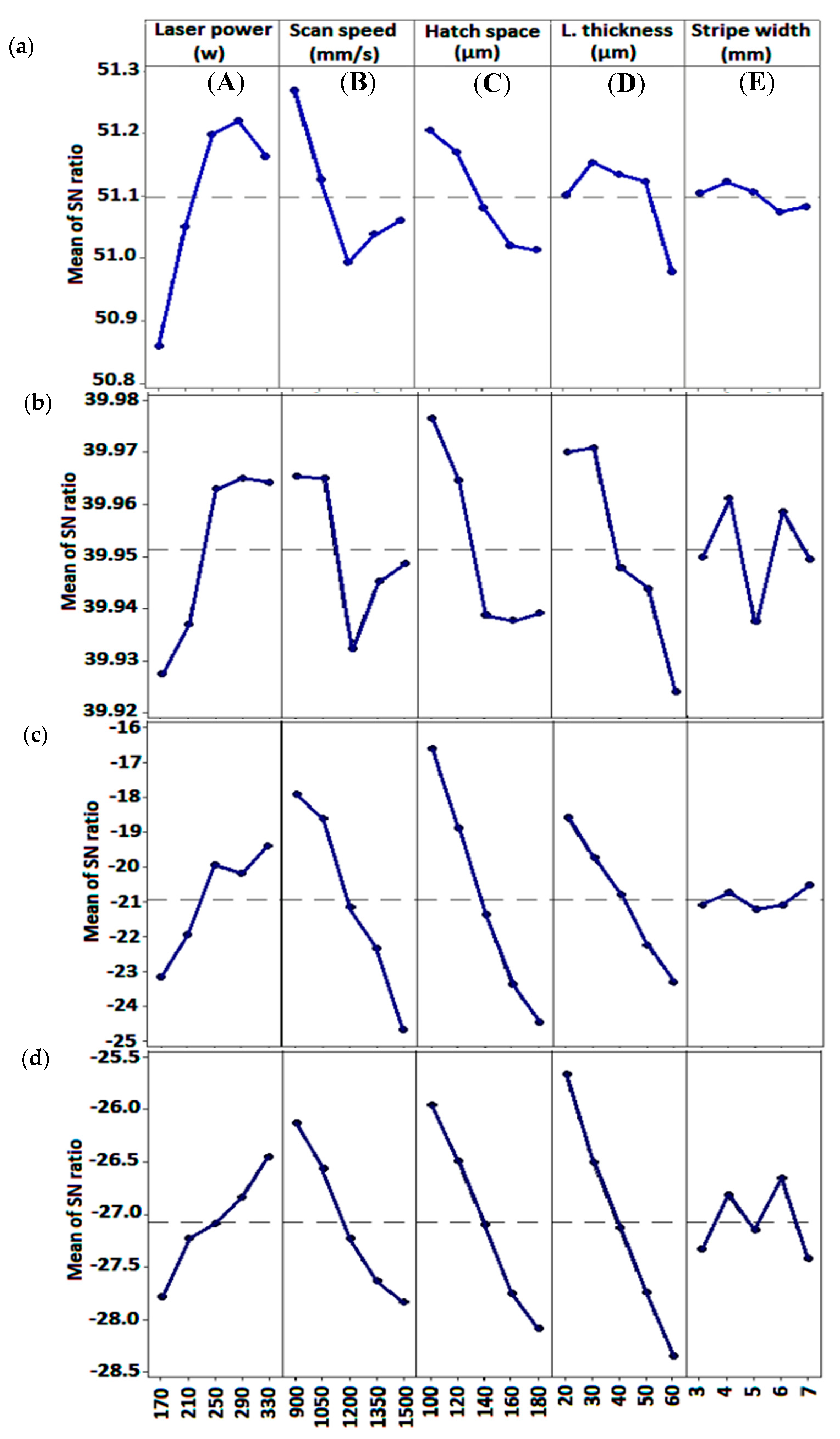
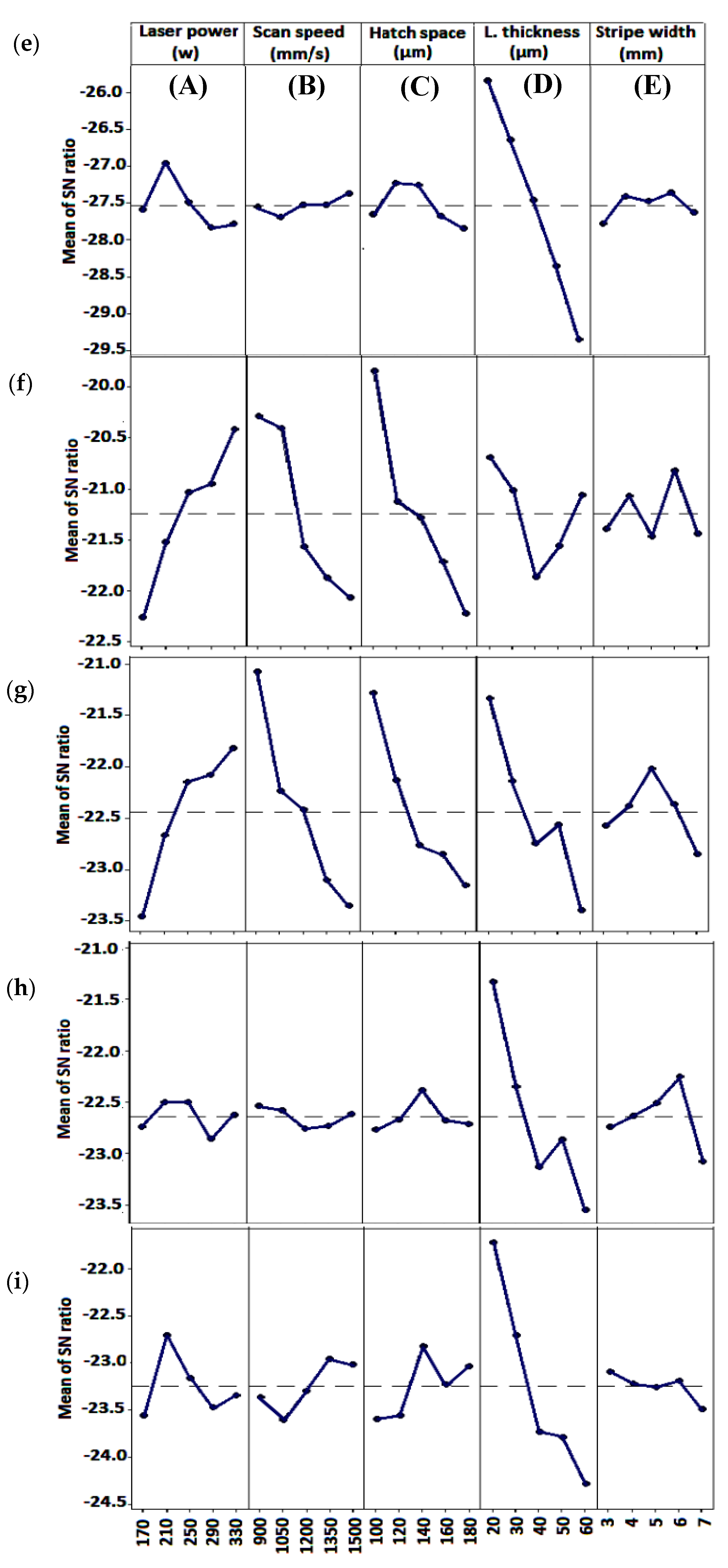
All the raw measurements for all the L-PBF process parameters listed in Table A1 and Table A2 are presented in Table A3 in the appendix. In the next sub-sections, the Taguchi, RSM, and ANN calculations and discussions are presented.

4.1. Taguchi Method

MSD values were calculated using Equations (2) and (3), depending on the measured property: minimization (Equation (2)) for roughness values and maximization (Equation (3)) for density and microhardness values. Hereafter, we refer to these desired values (higher or lower depending on the property) as the optimum values for simplicity. With the MSD values, the S/N ratios were calculated using Equation (1). Figure 3a–i shows the S/N ratios of different factors (A to E) and for different properties (e.g., microhardness and relative density). Every single point on the S/N ratio graph for each factor at each level was the average of the S/N ratios of all the samples manufactured using that factor at that level. For instance, the value of the first point on the left of the graph shown in Figure 3a was the mean S/N ratio of microhardness of all the samples manufactured using a laser power of 170 W.
As previously mentioned, a high S/N ratio is always desired. Therefore, the combination of the parameters that led to the optimum response was obtained by collecting the level of each factor that resulted in the highest S/N ratio for that response. For instance, Figure 3a shows that using the A4-B1-C1-D2-E2 combination of the factors resulted in the highest microhardness value in the given range of the process parameters. This combination corresponds to L-PBF process parameters of p = 290 W, v = 1200 mm/s, h = 100 µM, t = 30 µM, and d = 4 mm.
Table 2 lists the combinations of the L-PBF processing parameters that resulted in the optimum values for all the considered properties based on the S/N ratio plots shown in Figure 3. To investigate the contribution of each factor to the total variation in the response, analysis of variance (ANOVA) was performed. The p-values and contributions of the factors on different responses based on ANOVA linear regression results are presented in Table 3.
In statistical hypothesis testing, a p-value or probability value is the probability under a specified model that a statistical measurement of the data would be equal to or greater than its observed value. Hence, the p-value is the probability of observing test output values at least as high as the values obtained during the actual test, while the so-called “null hypothesis” is presumed to be correct [60]. The null hypothesis often presumes the lack of influence, such as a correlation between a parameter and a response. Therefore, a p-value gives the ability to evaluate the incompatibility between a factor and a proposed model for the data. Smaller p-values show a greater statistical incompatibility of the data with the null hypothesis, meaning a greater significance of the factor for the model. The percent contribution for any parameter was calculated by dividing the sum of squares for that factor by the total sum of squares of all factors and multiplying the result by 100 [27]. The last column of Table 2 summarizes the ANOVA results by ranking the contributions of the factors on the response from the highest to the lowest. The significance of the contribution of each factor to the response can also be inferred from the S/N ratio plots. The factors with higher variations in the S/N ratios have a higher influence on the related response. This behavior is proportional to the contributions of the factors, which are inversely proportional to their p-values shown in Table 3. For instance, factor A (laser power) was the most significant factor, with a 45.3% contribution in predicting the microhardness. The next factors in order of significance were B (23%), C (13.9%), D (7.9%), and E (0.7%).
The results presented in Figure 3 and the last column of Table 2 and Table 3 suggest that the influence of factor D (layer thickness) on all three downskin roughness responses was greater than the influence of all the other four considered factors, i.e., the contributions of all the other factors to the three downskin roughness responses were less than 10%. In all three cases, the optimum layer thickness was the smallest considered layer thickness, which was 20 µM. This observation showed that layer thickness-related mechanisms, such as stair-stepping, were the dominant factors influencing the downskin roughness in the L-PBF process. Debroy et al. [61] reported the same behavior for the surface of L-PBF-manufactured parts. Thus, based on Taguchi analysis, the smallest possible layer thickness was desired in the L-PBF process to minimize the downskin surface roughness. However, there are other considerations for the L-PBF process to set the lower limit of the layer thickness, such as manufacturing time, the upper limit of the powder size distributions, and powder-bed distortion due to the inert gas flow. To optimize the other four factors to achieve optimum downskin roughness, a reasonably small layer thickness must be chosen based on the considerations mentioned above and the tolerable downskin roughness. Then, another DoE, such as Taguchi, with the remaining four factors must be performed to determine the optimum L-PBF processing parameters. Generally, to improve the downskin roughness response, it is expected to have energy densities that are lower than the energy density corresponding to the optimum bulk properties such as relative density or microhardness. The slower cooling mechanism for the downskin compared to the bulk of the part confirms this expectation, i.e., the cooling mechanism changes from faster full conduction through the build plate to partial conduction through the build plate and partial convection through the downskin. On the other hand, at each layer, the laser beam penetrates some lower layers, and in downward-facing surfaces, a beam with very high energy densities absorbs and partially melts surrounding powder particles. This results in these particles attaching to the surface and increasing the roughness. Therefore, the levels of the factors need to be adjusted to result in lower energy densities for the new DoE.
Similar analogies and conclusions apply to the upskin roughness values regarding the role of the layer thickness. However, the layer thickness was not the only factor influencing the upskin roughness values. The hatch spacing, scanning speed, and laser power were the three other factors significantly contributing to the upskin roughness values; this fact also applied to the top surface roughness values. This three-factor combination effect suggests that the chosen ranges of the levels were sufficient to optimize the upskin and top surface roughness given a fixed layer thickness chosen based on the tolerable downskin roughness responses. Interestingly, the optimum factors for all three considered upskin roughness parameters and the top surface roughness were identical: p = 330 W, v = 900 mm/s, and h = 100 µM. These optimum parameter levels correspond to the limits of the levels that result in the highest energy density (183.3 J/mm3) considering all the combinations of the tested levels, i.e., the highest considered laser power and the lowest scanning speed and hatch spacing. Consequently, it can be concluded that the Taguchi method recommends the highest energy density level to obtain the smallest roughness values for the upskin and top surface roughness of L-PBF-manufactured parts. This is in contrast with the findings related to the optimum downskin roughness values where lower values of energy density (~55 J/mm3) correspond to the optimum downskin roughness values. A possible explanation for this observation may be offered by considering the gravitational force that smooths the melt lines on the top and upskin surfaces while coarsening the melt lines that are unsupported for downskin surfaces.
The L-PBF process parameters corresponding to optimum microhardness and relative density responses were identical: p = 290 W, v = 900 mm/s, h = 100 µM, t = 30 µM, and s = 4 mm. However, the significance of the factors and their contributions were different for these responses, suggesting that they were influenced by different mechanisms. The significant factors influencing relative density were laser power (22.6% contribution), scanning speed (14.1% contribution), hatch spacing (23.5% contribution), and layer thickness (28.0% contribution), and there was a slight contribution from stripe width (6.2% contribution). This conclusion from the ANOVA results is in good agreement with several past observations suggesting that relative density is qualitatively correlated with energy density with collective contributions from p, v, h, and t. Bartolomeu et al. [27] reported an increase in relative density by increasing energy density. Also, Sun et al. [62] observed a sharp increment of relative density by increasing energy density due to a decrease in layer thickness. The reported trend in the literature was valid here too, wherein an increase in energy density dramatically increased the relative density due to the removal of the lack of fusion defects to a maximum value, which was followed by a slight decrement due to the creation of entrapped gas porosities at higher energy densities. This phenomenon was evident when considering the S/N ratio behavior for the relative density response in Figure 3b. In this case, there was a sharp increase followed by a slight decrease in the S/N ratio in response to increasing the laser power and decreasing the layer thickness and scanning speed. The S/N ratio for the h factor was an exception, which increased monotonically by decreasing its levels. Finally, the stripe width had a small contribution to the relative density. It appeared that the contribution of stripe width to the total defects in the part was closer to the outer boundary of the parts where the complete stripe width was not observed. For these incomplete stripe width scans, the cooling time before scanning the adjacent line was shorter, which may result in higher energy density and entrapped gas porosities.
Regarding the microhardness response, the correlation explained for energy density and relative density was roughly valid. However, only three factors had a meaningful contribution to the microhardness response. Laser power was the dominant factor (45.3% contribution) influencing the microhardness response, followed by scanning speed (23.3% contribution) and hatch spacing (13.9% contribution). However, the contributions of layer thickness and stripe width were less than the error in the ANOVA (8.8%) for this response and therefore considered insignificant. The dominance of laser power on the microhardness response was an interesting observation that was not justified regarding the energy density factor. According to research done by Calignano et al. [15], a possible explanation can be offered by considering the significant influence of laser power on the fluid flow and recoiling pressure inside the melt-pool. As the laser power increased, the fluid flow inside the melt-pool became stronger, resulting in a more homogenous solid solution after solidification that in turn increased the microhardness. As the laser power increased further, the recoiling pressure increased, resulting in the collapse of the melt-pool and creating defects that in turn decreased the microhardness. Furthermore, the microhardness was determined by Vickers indentations on cross-sections of the parts in the XY direction, with indentation diagonals of ~70 µM, which was larger than the thickness of the thickest layer. Therefore, a single indentation, regardless of the layer thickness, always included more than one layer and was thus always affected by the partial interlayer bonding. This explains the negligible influence of the layer thickness on the microhardness response. Finally, the microhardness indentations were performed away from the boundaries where the contribution of the stripe width on densification was significant; this fact justified the observed insignificant influence of stripe width on the microhardness response.

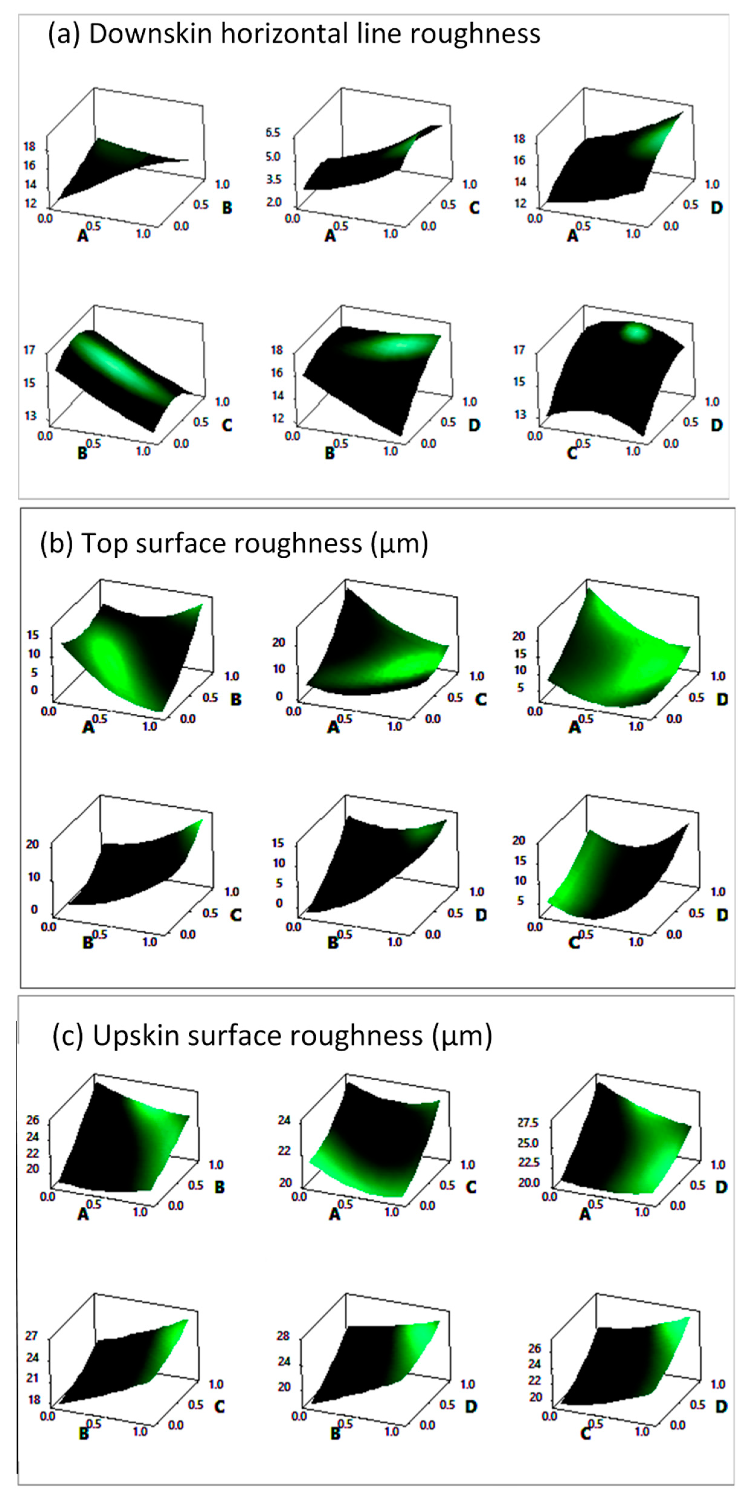
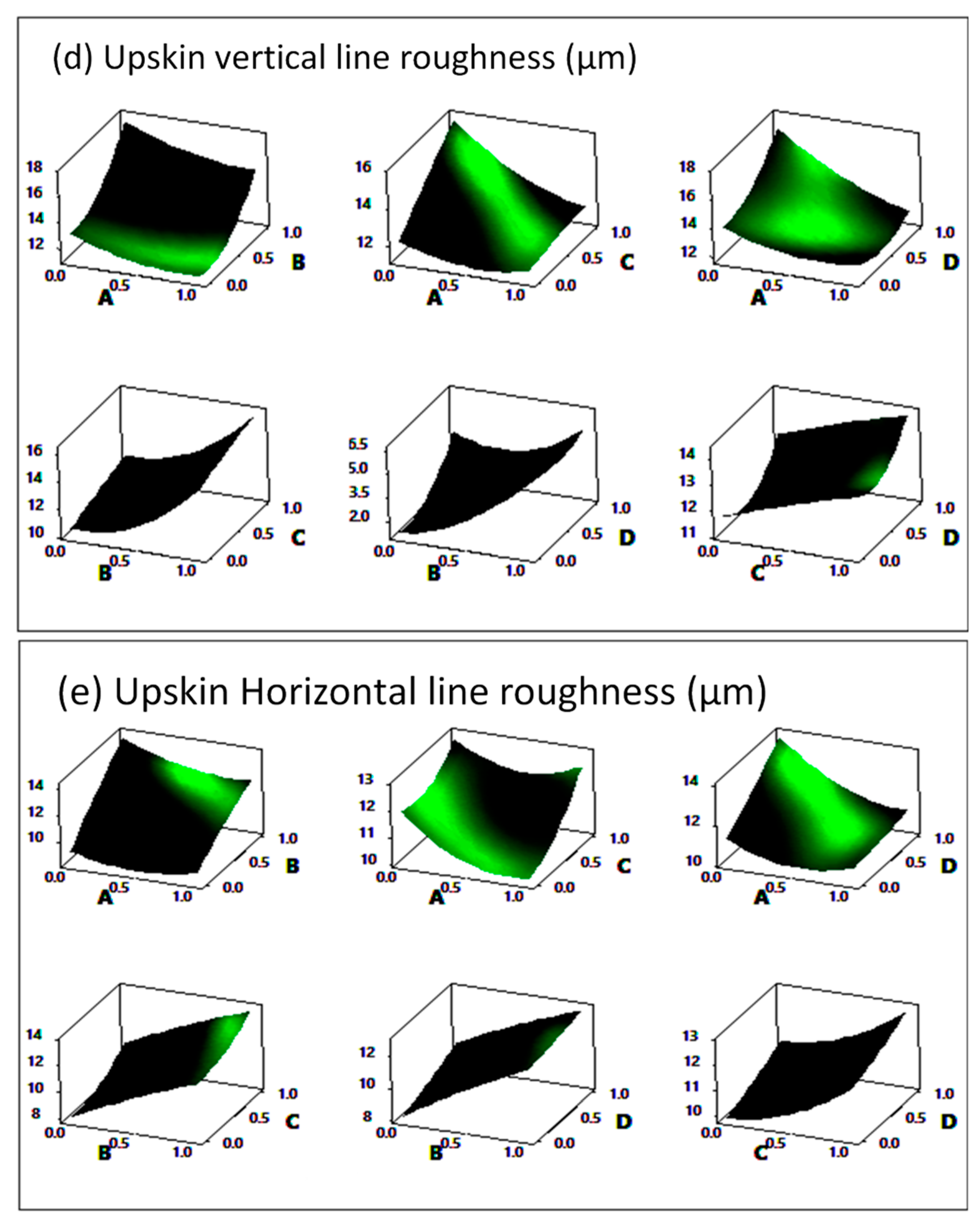
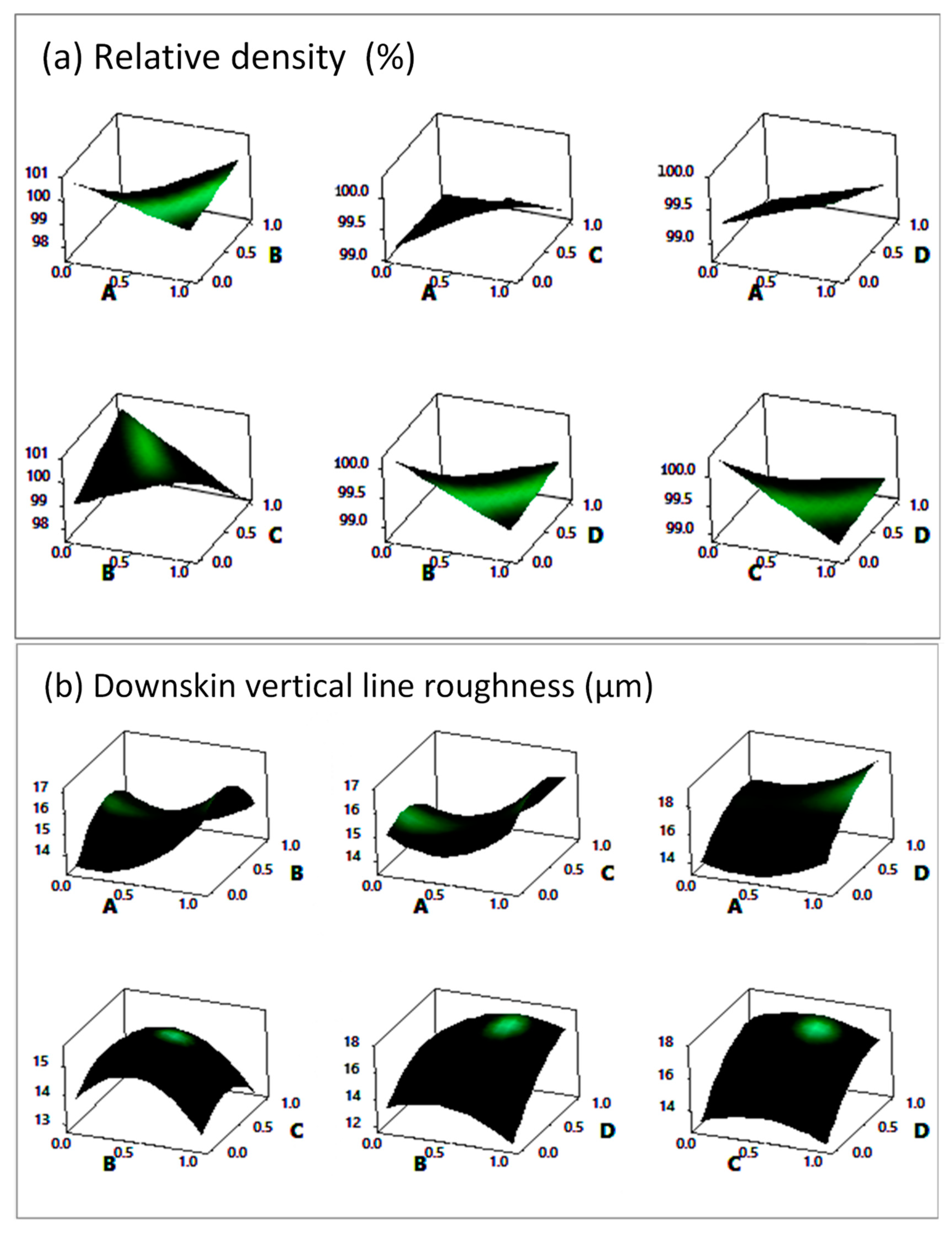
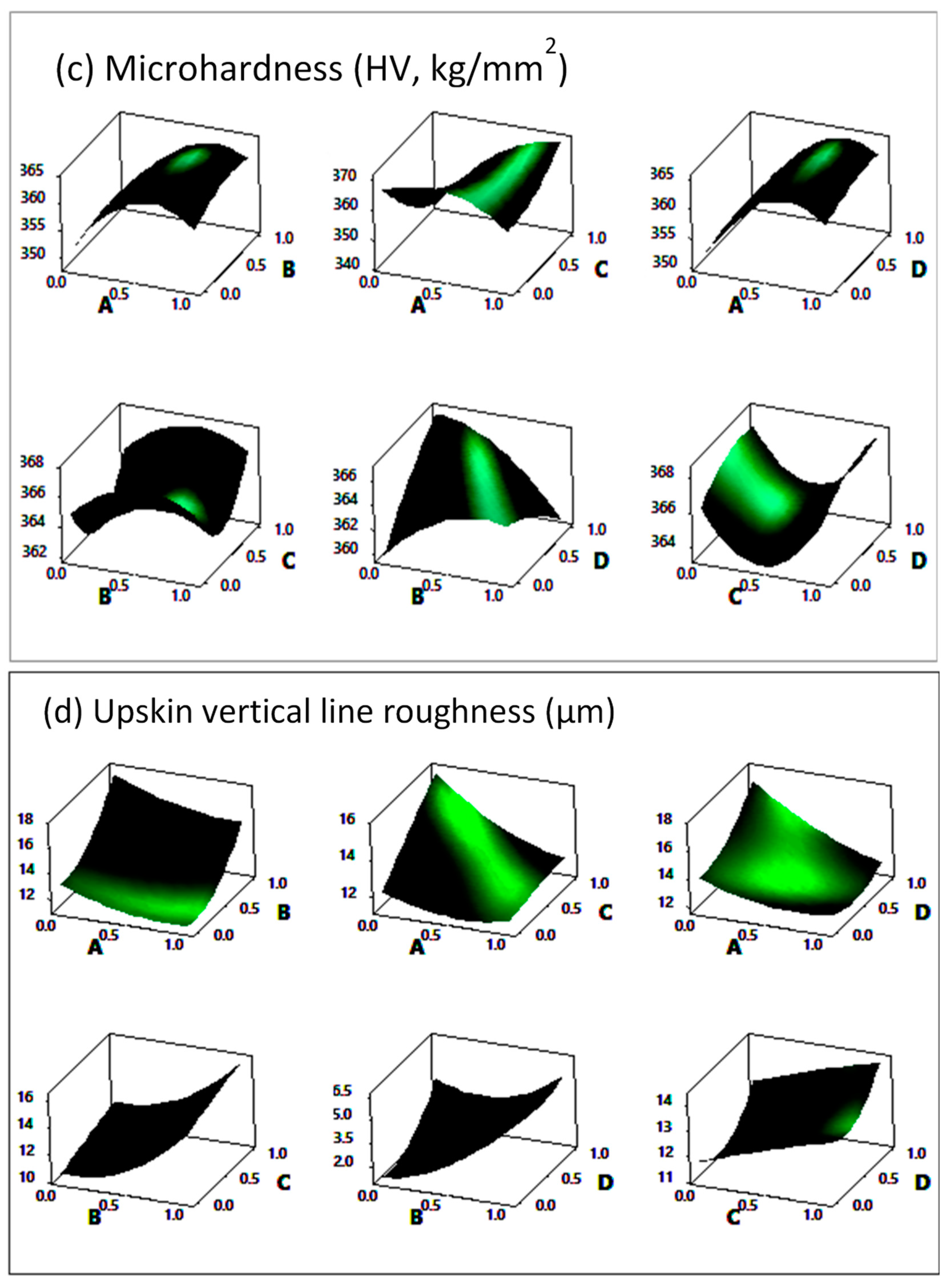
4.2. Response Surface Method

Quadratic models were fitted to Equation (6) to calculate the coefficients ( β i ) for each property. The parameter values were normalized before being used for regression. Table 4 presents the coefficients of the response surface equation of each property (e.g., microhardness) as functions of linear, two-way interaction, and quadratic terms of process parameters. To evaluate the significance of each coefficient, p-values obtained from the ANOVA of quadratic response surface regression for different responses are listed in Table 5. Response surface plots are very useful to evaluate the interaction effects between two parameters in a DoE study. Figure 4 and Figure A1 in the appendix illustrate the response surface plots of each two-parameter combination when the other two parameters were kept constant at their default values, which are presented in the lower right section.
Since normalized parameters were used to form the response equations, the magnitude of their coefficients (Table 4) was an indication of their significance in predicting the response. The response equation obtained for each property can be used to visualize the variations in that response versus the variations in two predictors at a time. Therefore, the rest of the factors should be kept constant when plotting the response surface. Any convolution on the surface plot indicates that the variation in one factor alters the behavior of the other factor. For instance, in Figure 4c, the interaction between laser power and hatch spacing, i.e., the AC plot, shows that when laser power (A) was at its highest level, by increasing the hatch spacing (C), the microhardness value increased; however, when laser power (A) was at its lowest level, the microhardness decreased with increasing hatch spacing (C). Therefore, it can be said that the effect of laser power on microhardness depends on the hatch spacing level. This surface was the most convoluted surface among the microhardness response surfaces (Figure 4c), indicating that these two parameters—laser power and hatch spacing—were the most correlated factors in predicting the microhardness of the fabricated parts. This conclusion can be supported by comparing the coefficient (2nd column of Table 4) and contribution percentage (3rd column of Table 5) of AC with the other interactions, i.e., AB, AD, and BD.
The contribution percentage of the AC interaction in predicting microhardness was 13.9%, which is higher than 0.3%, 0.4%, and 2.2% for AB, AD, and BD, respectively. A similar significance of AC to the other parameter interactions can be seen in predicting the relative density and top surface roughness (Figure 4a and Figure A1b, Table 4 and Table 5). Figure 4a illustrates that the effects of laser scanning speed on relative density at high levels of laser power were negligible; however, when the laser power was low, the response decreased sharply with increasing scanning speed. The interaction of scanning speed and layer thickness in predicting microhardness and relative density (BD interaction) in Figure 4a,c shows that at a low layer thickness, e.g., 20 µM, microhardness increased and relative density decreased in response to increases in the laser scanning speed. However, when the layer thickness was high, increasing the scanning speed had the opposite effect: decreasing the microhardness and increasing the relative density. These behaviors can be justified by considering the optimum values of these properties versus energy density. For instance, take microhardness behavior versus energy density as an example. A low layer thickness generally results in a high energy density (higher than the optimum value that gives the maximum microhardness value), so increasing the scanning speed increased the microhardness toward the maximum value. However, high layer thickness values lead to energy densities lower than the optimum value, so increasing the scanning speed, i.e., decreasing the energy density, decreased the microhardness away from the maximum value.
Table 5 shows that in contrast to microhardness and relative density, in the upskin roughness properties, the interaction between laser power and layer thickness (AD interaction) was the most significant. Figure 4d and Figure A1c,e illustrates this by showing changes in the effect of one parameter on the response when the other parameter was varied. In these cases, when the laser power was low, the roughness value increased drastically with increasing layer thickness, whereas it did not change with increasing layer thickness at high levels of laser power. As described by Fotovvati et al. [63], who critically reviewed melt-pool characteristics in laser welding of metals, this may be ascribed to the fact that high laser powers form deeper melt-pools which penetrate deeper and melt the previously deposited layers regardless of their thickness, concealing the effects of layer thickness on roughness values. However, this is not the case for downward-facing surfaces. Increasing the layer thickness increases the roughness, regardless of the other parameters. This can be verified by the interaction of layer thickness with other parameters (AD, BD, and CD interactions in Figure 4b and Figure A1a,d).
This behavior can be due to the stair-stepping effect, as previously discussed, and it is confirmed by being less observable in downskin horizontal line roughness than in downskin surface roughness and downskin vertical line roughness responses. By comparing the p-values and contribution percentages of quadratic terms with the linear ones in the responses, the behavior type of each response can be realized. For instance, in the proposed model for upskin surfaces, the contribution percentages of the quadratic terms were negligible compared to the linear ones. Additionally, the related response surface presented in Figure 4d and Figure A1c,e exhibited smaller curvature than the other response surfaces. Therefore, since the R2 values of these response equations were relatively high (Table 5), it can be concluded that modeling the upskin roughness parameters using a linear model can be less expensive without missing any significant quadratic effect of the main factors and their interactions.
Response optimization helps to identify the variable settings that optimize a response. Table 6 presents the parameter settings that minimize/maximize each of the response equations (Table 4) along with the optimized responses, which can be obtained using those parameter combinations. The standard error of the fit (SE fit) evaluates the fluctuation in the predicted mean output value for the specified parameter combination and is used to calculate the confidence interval (CI) for the mean response. The 90% CIs are ranges of values that have a 90% probability of containing the mean output value for the population with the obtained values of the parameters in the model.
Table 6 shows that the smallest layer thickness was recommended to achieve superior roughness parameters on all the surfaces investigated in this research. This was consistent with the Taguchi recommendation (Table 2). Similar to the Taguchi optimization, larger values of energy density were recommended for upward-facing surfaces, i.e., top and upskin, rather than for downskin roughness parameters. According to the information presented for the roughness values in Table 6 (columns A and B), the factors can be classified into two groups: (1) downskin surface and vertical line roughness and (2) other surface properties. The recommended scanning speed values for the former were higher than those for the latter. This was also consistent with the Taguchi results.
A parameter combination that is best for one response does not necessarily optimize the other properties. A multi-response optimization can obtain a parameter setting that optimizes all the properties considering their weight. The multi-response optimization of all nine properties (with the same weights) studied in this research is presented in Table 7. The results showed that each of the response values from this multi-response optimization was slightly worse than the ones obtained for their individual optimization. This is a compromise for having all of them optimized using a single set of input parameters. It is worth mentioning that this approach can be implemented with different weights for different responses based on the importance of each response to the specific application of the L-PBF-manufactured component.

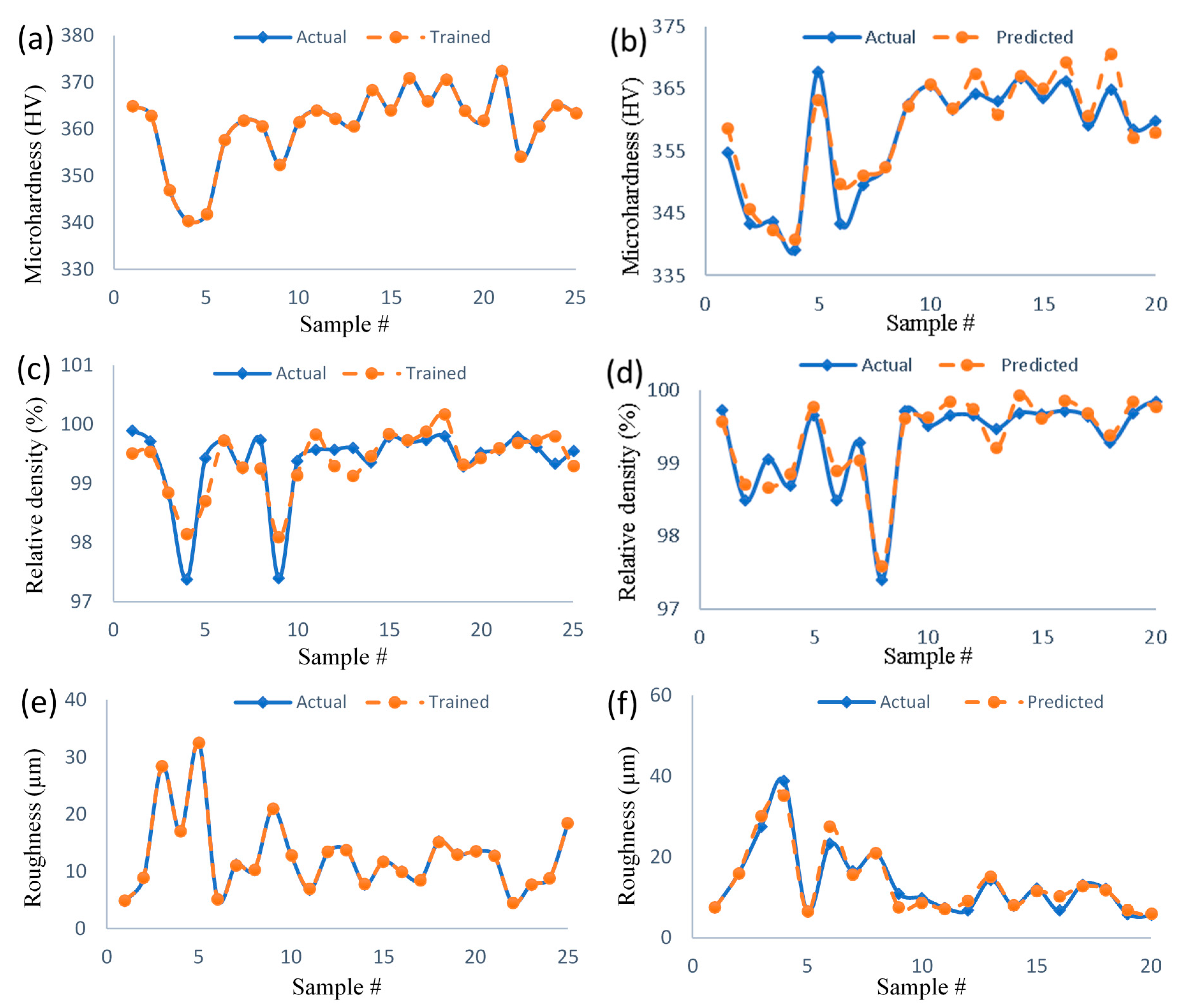
4.3. Artificial Neural Network

After the ANN was trained, all the data were fed to it, and the predictions were compared to the actual values to validate the ANN model. Figure 5 illustrates a comparison of the microhardness, relative density, and roughness training and testing results. The trained ANN models exhibited good accuracy and performance. A quantitative comparison between the predictive accuracy of the network and the other two employed methods is presented next. The weight and bias values of the neural network are presented in Table A4, Table A5 and Table A6 in Appendix A.

4.4. Comparison of the Predictions from the Taguchi Method, the Response Surface Method, and the Artificial Neural Network

To compare the performance of the three proposed methods, 20 new parameter combinations (unseen data) were used as input to each model, and the output was considered to be the predicted response. The difference between the predicted and actual responses was divided by the actual value to obtain the error for each of the 20 unseen data points. The mean absolute values of these errors were then calculated for each response property and for all of them, the results of which are presented in Table 8. According to the results, the Taguchi method showed the largest mean absolute error values in predicting each and all the response properties. This verified that there were nonlinear behaviors in the responses that the Taguchi method was not able to capture as accurately as the quadratic models. Considering the microhardness prediction error values, the RSM performed slightly better than the ANN; however, the ANN showed much better performance in predicting the other properties of the unseen samples. The ANN also had a much lower total mean absolute error than the other two methods, making it superior in terms of the overall performance.

5. Conclusions

In this study, three methodologies were presented to determine five L-PBF processing parameters—laser power, scanning speed, hatch spacing, layer thickness, and stripe width—to optimize nine performance responses—relative density, microhardness, and six line and surface roughness parameters for the top, upskin, and downskin surfaces. First, the application of the Taguchi method and the RSM for the DoE in determining the L-PBF processing parameters to achieve optimum properties was presented. Furthermore, a feed-forward back-propagation ANN with six and five nodes in two hidden layers was established using the Bayesian regularization method for predicting the responses of the L-PBF-manufactured samples. Fractional prediction error for the ANN was calculated and compared to the similar values for the Taguchi and RSM. The major conclusions of this article are:
  • Both Taguchi and RSM approaches were successful in capturing the correlations between the L-PBF processing parameters and responses by using only 1/125th of the observations in full factorial experiments.
  • The Taguchi results showed that the layer thickness was the most significant factor in determining all the three downskin roughness responses, in which the optimum layer thickness was the smallest value, i.e., 20 µM. Therefore, the layer thickness-related mechanisms, such as stair-stepping effect, were the dominant factors influencing the downskin roughness in the L-PBF process.
  • The Taguchi method recommends the highest energy density level to obtain the smallest roughness values for the upskin and top surface roughness of L-PBF-manufactured parts, regardless of all the other properties.
  • Similarly, the parameter combinations recommended by the RSM resulting in the smoothest up-facing surfaces in L-PBF-manufactured parts yields the highest energy densities.
  • Using RSM results, we were able to assess whether two input parameters are independent in determining a response. The results showed that the interaction between the laser power and hatch spacing in predicting microhardness and relative density was the most significant among the two-way interactions between the other parameters. However, in the upskin roughness properties, the most significant interaction was between laser power and layer thickness.
  • A multi-response optimization of all nine properties with the same weights is performed to obtain a single set of L-PBF processing parameters for optimizing all the response properties. The applied weight on each response can be altered based on their importance to the specific application of the L-PBF-manufactured component.
  • Overall, the present analyses by both Taguchi and RSM methods showed that the layer thickness was the dominant factor controlling the downskin surface roughness parameters and was a significant factor influencing the top surface and upskin roughness parameters.
  • The contribution of stripe width on most responses was negligible, which was attributed to its local importance near the boundaries of parts.
  • The microhardness and relative density were both influenced by the energy density calculated based on the laser power, scanning speed, layer thickness, and hatch spacing. However, laser power played a more dominant role on the microhardness response than on the relative density response.
  • The trained ANN model exhibited very good accuracy and performance in predicting the true response values based on the given input processing parameters.
  • The comparison of the prediction errors corresponding to the ANN, the RSM, and the Taguchi method showed that all the three models exhibited reasonable predictive capabilities.
  • Among the three models, the Taguchi method showed the least desirable performance in predicting each and all the response properties. We can conclude that nonlinearity exists in the behavior of the tested response properties of PBF-manufactured parts that the Taguchi method was not able to capture as accurately as the quadratic models.
  • Although the RSM performed slightly better than the ANN in predicting microhardness values, the ANN showed much better performance in predicting the other properties. Therefore, it can be concluded that the ANN outperformed the predictive capabilities of the RSM and the Taguchi method.

Author Contributions

B.F. wrote the manuscript with significant contributions from E.A., M.B. contributed to ANN modeling, writing, and analysis. E.A. and B.F. collaboratively designed the research, while B.F. implemented the methods. E.A. supervised the entire research. All authors have read and agreed to the published version of the manuscript.

Funding

This material was based upon work supported by the Naval Air Station Patuxent River (MD 20670-1906) under contract N6893620C0022 through a subcontract from MRL Materials Resources LLC. This work was also partially funded through the Technology Development Grant by the FedEx Institute of Technology.

Conflicts of Interest

The authors declare no conflict of interest. The funders had no role in the design of the study; in the collection, analyses, or interpretation of data; in the writing of the manuscript, or in the decision to publish the results.

Appendix A

Table A1. The L25 Taguchi orthogonal array for five factors and five levels.
Experiment No.Processing Parameter Level
ABCDE
100000
201111
302222
403333
504444
610123
711234
812340
913401
1014012
1120241
1221302
1322413
1423024
1524130
1630314
1731420
1832031
1933142
2034203
2140432
2241043
2342104
2443210
2544321
Table A2. Fractional factorial design for five five-level factors.
Experiment No.Processing Parameter Level
ABCDE
100000
201123
302241
403314
504432
610111
711234
812302
913420
1014043
1120222
1221340
1322413
1423031
1524104
1630333
1731401
1832024
1933142
2034210
2140444
2241012
2342130
2443203
2544321
Table A3. Raw data of all the experiments carried out for this research.
Sample Code *Relative Density (%)Hardness (HV)Roughness (µm)
Top Surface Upskin Surface Upskin Hor. LineUpskin Ver. LineDownskin SurfaceDownskin Hor. LineDownskin Ver. Line
1111199.893364.914.8616.639.149.8520.5212.1812.99
1222299.726354.807.5419.5511.6213.8619.7313.0014.63
1223499.712362.838.8521.9711.7914.6520.8512.0715.31
1333398.493343.4015.8623.7213.7214.6722.3013.2815.08
1335298.824346.9128.4227.7913.3016.2724.7014.7915.61
1442597.379340.3317.0924.4612.7515.9520.3014.0014.64
1444499.053343.7427.5230.0815.0317.0926.7313.2715.07
1554399.431341.8032.5232.2717.1221.5228.1815.5415.10
1555598.685339.1838.8438.1916.8321.4432.7417.3618.02
2122299.732357.645.2618.967.7412.6623.6415.2613.14
2123499.650367.696.5219.4811.3511.7422.5714.4516.37
2234599.258361.8211.2324.0211.1514.5124.2914.1414.68
2341399.734360.6110.2618.6910.6712.5216.6311.0011.58
2345198.493343.423.3030.0413.6316.5827.0315.0214.56
2451299.277349.5416.5121.2112.1313.4418.2911.0210.65
2453197.399352.4020.9826.7713.6514.8424.7014.9916.37
2512399.712362.5210.9321.4711.4912.2720.3212.4812.77
2515499.383361.5312.8326.6314.1115.2125.4816.4515.91
3133399.571363.986.8119.678.2211.0324.4814.5214.85
3135299.503365.489.8123.6110.0412.7028.4713.8115.31
3241399.650361.677.4220.8710.9411.2121.5812.1513.66
3245199.573362.2013.3925.3111.6215.7127.5915.3716.12
3352499.602360.5913.7222.6911.7513.1621.5512.8513.07
3413599.646364.186.7922.1111.8613.4822.6014.9715.11
3414299.358368.307.7426.4312.1713.8727.1316.5216.63
3521599.789364.0211.7425.0012.5917.8019.4112.1911.94
3524199.470363.0514.3823.9911.8613.6424.8113.0714.98
4142599.684366.777.9619.369.6811.1222.3913.2314.40
4144499.702370.839.9522.4311.5512.3229.1418.4616.36
4251299.735365.988.5423.5411.3614.1424.1514.6613.68
4253199.669363.4412.1724.9412.7814.2727.0914.5015.44
4313599.801370.5615.2419.0210.3510.4624.9314.9715.63
4314299.714366.286.7821.7410.5511.4129.1615.8217.98
4425399.286363.9213.0025.1611.5013.9128.9615.7016.69
4531499.632359.0713.1119.3711.5313.1617.7910.9011.07
4532199.516361.7513.5523.3611.8314.9323.5813.7513.48
5154399.283364.9212.1622.9611.7311.3726.2113.4014.84
5155599.570372.4412.7825.8110.3713.2731.3917.7815.67
5212399.787354.084.4917.818.1810.4926.9615.3814.29
5215499.681358.515.8317.926.9711.2529.8713.6517.58
5321599.830359.805.6918.2910.6411.0520.0412.1012.96
5324199.615360.617.6925.3211.8813.6239.5920.2220.96
5431499.338365.068.8922.7612.1313.5124.0014.2316.04
5432199.600361.159.5522.8311.8113.8123.7414.0213.58
5543299.551363.4218.4623.8112.4114.6323.7614.6114.91
* Sample code is a five-digit code that each digit, from left to right, is representative for the level of factors A, B, C, D, and E, respectively, as shown in Table 2. For instance, the factor levels of the sample 12234 are A1, B2, C2, D3, and E4.
Table A4. Weight and bias values applied to the input layer of the neural network.
WeightBias
−0.8172269311.2743454058−0.4373294332−0.25438937580.0672884998
−0.17427198030.0407326757−0.9436160018−0.0765179160.7709497912
0.46185497110.1455196574−0.2580787273−0.8655356556−0.1703290546
0.44209872840.90075289461.0511498950.71401463120.5015783122
0.9768443561−0.4022851406−0.6007116257−0.0787949740.9597908008
0.3804623429−0.86450488490.279432945−0.47447033920.5012114738
Table A5. Weight and bias values applied to the first hidden layer of the neural network.
WeightBias
0.69163044−0.29082017−0.689155160.016574950.530584970.62056222−0.29844372
−0.49439060.56887031−0.02349223−0.7047001−1.191402180.17356839−0.17197129
−0.1946129−0.094545160.01747523−1.29675660.125823570.47763527−0.12213046
0.226372720.11649799−0.096554290.84722914−0.746405280.25596798−0.30446552
−0.25275280.7461884960.8990364940.833783850.256524716−0.0999083−0.0819088467
Table A6. Weight and bias values applied to second hidden layer of the neural network.
WeightBias
−0.0951860163−0.58475616820.2450872866−0.5658932656−0.07128147030.280699756
0.8474751074−1.33452361560.6504012392−0.39313963630.0672525452−0.47777086
−0.9487583799−0.3165275189−0.8272228144−0.5577874479−1.0364007486−0.26500424
Figure A1. Response surface plots of each two-parameter combination for (a) downskin horizontal line roughness, (b) top surface roughness, (c) upskin surface roughness, (d) downskin surface roughness, and (e) upskin horizontal line roughness. Constant parameters kept at: A (laser power) = 280 w, B (scan speed) = 1200 mm/s, C (hatch spacing) = 140 µM, and D (layer thickness) = 30 µM. Each surface shows the variations of the response (vertical axis) versus variations of two process parameters (horizontal axes) at a time, while the other two parameters are kept constant at their default values mentioned in the figure legend. For simplicity, and to increase the figure readability, the parameter values are normalized as 0 represents the value of the first level and 1 represents the value of the highest level.
Coatings 10 01104 g0a1aCoatings 10 01104 g0a1b

References

  1. Qiu, C.; Al Kindi, M.; Aladawi, A.S.; Al Hatmi, I. A Comprehensive Study on Microstructure and Tensile Behaviour of a Selectively Laser Melted Stainless Steel. Sci. Rep. 2018, 8, 1–16. [Google Scholar] [CrossRef]
  2. Charles, A.; Elkaseer, A.; Thijs, L.; Hagenmeyer, V.; Scholz, S.G. Effect of Process Parameters on the Generated Surface Roughness of Down-Facing Surfaces in Selective Laser Melting. Appl. Sci. 2019, 9, 1256. [Google Scholar] [CrossRef] [Green Version]
  3. Perevoshchikova, N.; Rigaud, J.; Sha, Y.; Heilmaier, M.; Finnin, B.; Labelle, E.; Wu, X. Optimisation of Selective Laser Melting Parameters for the Ni-Based Superalloy IN-738 LC Using Doehlert’s Design. Rapid Prototyp. J. 2017, 23, 881–892. [Google Scholar] [CrossRef] [Green Version]
  4. Fox, J.C.; Moylan, S.P.; Lane, B. Effect of Process Parameters on the Surface Roughness of Overhanging Structures in Laser Powder Bed Fusion Additive Manufacturing. Procedia CIRP 2016, 45, 131–134. [Google Scholar] [CrossRef] [Green Version]
  5. Chen, Z. Understanding of the Modeling Method in Additive Manufacturing. IOP Conf. Ser. Mater. Sci. Eng. 2020, 711. [Google Scholar] [CrossRef]
  6. Fisher, R.A. Design of Experiments. BMJ 1936, 1, 554. [Google Scholar] [CrossRef]
  7. Nath, R.; Murugesan, K. Optimization of Double Diffusive Mixed Convection in a Bfs Channel Filled With Alumina Nanoparticle Using Taguchi Method and Utility Concept. Sci. Rep. 2019, 9, 1–19. [Google Scholar] [CrossRef]
  8. Liu, Y.; Liu, C.; Liu, W.; Ma, Y.; Tang, S.; Liang, C.; Cai, Q.; Zhang, C. Optimization of Parameters in Laser Powder Deposition AlSi10Mg Alloy Using Taguchi Method. Opt. Laser Technol. 2019, 111, 470–480. [Google Scholar] [CrossRef]
  9. Manjunath, B.; Vinod, A.; Abhinav, K.; Verma, S.; Sankar, M.R. Optimisation of Process Parameters for Deposition of Colmonoy Using Directed Energy Deposition Process. Mater. Today Proc. 2020, 26, 1108–1112. [Google Scholar] [CrossRef]
  10. Yang, B.; Lai, Y.; Yue, X.; Wang, D.; Zhao, Y. Parametric Optimization of Laser Additive Manufacturing of Inconel 625 Using Taguchi Method and Grey Relational Analysis. Scanning 2020, 2020, 1–10. [Google Scholar] [CrossRef]
  11. Cherkia, H.; Kar, S.; Singh, S.S.; Satpathy, A. Fused Deposition Modelling and Parametric Optimization of ABS-M30. In Advances in Materials and Manufacturing Engineering; Springer: Singapore, 2020; pp. 1–15. [Google Scholar]
  12. Dontsov, Y.V.; Panin, S.; Buslovich, D.G.; Berto, F. Taguchi Optimization of Parameters for Feedstock Fabrication and FDM Manufacturing of Eear-Resistant UHMWPE-Based Composites. Materials 2020, 13, 2718. [Google Scholar] [CrossRef]
  13. Jiang, H.-Z.; Li, Z.-Y.; Feng, T.; Wu, P.-Y.; Chen, Q.-S.; Feng, Y.-L.; Li, S.-W.; Gao, H.; Xu, H.-J. Factor Analysis of Selective Laser Melting Process Parameters With Normalised Quantities and Taguchi Method. Opt. Laser Technol. 2019, 119, 105592. [Google Scholar] [CrossRef]
  14. Campanelli, S.; Casalino, G.; Contuzzi, N.; Ludovico, A. Taguchi Optimization of the Surface Finish Obtained by Laser Ablation on Selective Laser Molten Steel Parts. Procedia CIRP 2013, 12, 462–467. [Google Scholar] [CrossRef]
  15. Calignano, F.; Manfredi, D.; Ambrosio, E.P.; Iuliano, L.; Fino, P. Influence of Process Parameters on Surface Roughness of Aluminum Parts Produced by DMLS. Int. J. Adv. Manuf. Technol. 2013, 67, 2743–2751. [Google Scholar] [CrossRef] [Green Version]
  16. Rathod, M.K.R.; Karia, M.M.C. Experimental Study for Effects of Process Parameters of Selective Laser Sintering for alsi10mg. Int. J. Technol. Res. Eng. 2020, 7, 6957–6960. [Google Scholar]
  17. Joguet, D.; Costil, S.; Liao, H.; Danlos, Y. Porosity Content Control of CoCrMo and Titanium Parts by Taguchi Method Applied to Selective Laser Melting Process Parameter. Rapid Prototyp. J. 2016, 22, 20–30. [Google Scholar] [CrossRef]
  18. Sathish, S.; Anandakrishnan, V.; Dillibabu, V.; Muthukannan, D.; Balamuralikrishnan, N. Optimization of Coefficient of Friction for Direct Metal Laser Sintered Inconel 718. Adv. Manuf. Technol. 2019, 371–379. [Google Scholar] [CrossRef]
  19. Dong, G.; Marleau-Finley, J.; Zhao, Y.F. Investigation of Electrochemical Post-Processing Procedure for Ti-6AL-4V Lattice Structure Manufactured by Direct Metal Laser Sintering (DMLS). Int. J. Adv. Manuf. Technol. 2019, 104, 3401–3417. [Google Scholar] [CrossRef]
  20. Kuo, C.-C.; Yang, X.-Y. Optimization of Direct Metal Printing Process Parameters for Plastic Injection Mold With Both Gas Permeability and Mechanical Properties Using Design of Experiments Approach. Int. J. Adv. Manuf. Technol. 2020, 109, 1219–1235. [Google Scholar] [CrossRef]
  21. Gunst, R.F.; Mason, R.L. Fractional Factorial Design. Wiley Interdiscip. Rev. Comput. Stat. 2009, 1, 234–244. [Google Scholar] [CrossRef]
  22. Dada, M.; Popoola, P.; Mathe, N.; Pityana, S.; Adeosun, S. Parametric Optimization of Laser Deposited High Entropy Alloys Using Response Surface Methodology (RSM). Int. J. Adv. Manuf. Technol. 2020, 109, 2719–2732. [Google Scholar] [CrossRef]
  23. Pant, P.; Chatterjee, D.; Nandi, T.; Samanta, S.K.; Lohar, A.K.; Changdar, A. Statistical Modelling and Optimization of Clad Characteristics in Laser Metal Deposition of Austenitic Stainless Steel. J. Braz. Soc. Mech. Sci. Eng. 2019, 41, 283. [Google Scholar] [CrossRef]
  24. Read, N.; Wang, W.; Essa, K.; Attallah, M.M. Selective Laser Melting of ALSi10Mg Alloy: Process Optimisation and Mechanical Properties Development. Mater. Des. 2015, 65, 417–424. [Google Scholar] [CrossRef] [Green Version]
  25. El-Sayed, M.A.; Ghazy, M.; Youssef, Y.; Essa, K. Optimization of SLM Process Parameters for Ti6Al4V Medical Implants. Rapid Prototyp. J. 2019, 25, 433–447. [Google Scholar] [CrossRef] [Green Version]
  26. Gajera, H.M.; Darji, V.; Dave, K. Application of Fuzzy Integrated JAYA Algorithm for the Optimization of Surface Roughness of DMLS Made Specimen: Comparison with GA. In Advances in Intelligent Systems and Computing; Springer Science and Business Media LLC: Amsterdam, The Netherlands, 2019; Volume 949, pp. 137–152. [Google Scholar]
  27. Bartolomeu, F.; Faria, S.; Carvalho, O.; Pinto, E.; Alves, N.; Silva, F.S.; Miranda, G. Predictive Models for Physical and Mechanical Properties of Ti6Al4V Produced by Selective Laser Melting. Mater. Sci. Eng. A 2016, 663, 181–192. [Google Scholar] [CrossRef]
  28. Krishnan, M.; Atzeni, E.; Canali, R.; Calignano, F.; Manfredi, D.G.; Ambrosio, E.P.; Iuliano, L. On the Effect of Process Parameters on Properties of AlSi10Mg Parts Produced by DMLS. Rapid Prototyp. J. 2014, 20, 449–458. [Google Scholar] [CrossRef]
  29. Pawlak, A.; Rosienkiewicz, M.; Chlebus, E. Design of Experiments Approach in AZ31 Powder Selective Laser Melting Process Optimization. Arch. Civ. Mech. Eng. 2017, 17, 9–18. [Google Scholar] [CrossRef]
  30. Marmarelis, M.G.; Ghanem, R.G. Data-Driven Stochastic Optimization on Manifolds for Additive Manufacturing. Comput. Mater. Sci. 2020, 181, 109750. [Google Scholar] [CrossRef]
  31. Wang, G.; Huang, L.; Liu, Z.; Qin, Z.; He, W.; Liu, F.; Chen, C.; Nie, Y. Process Optimization and Mechanical Properties of Oxide Dispersion Strengthened Nickel-Based Superalloy by Selective Laser Melting. Mater. Des. 2020, 188, 108418. [Google Scholar] [CrossRef]
  32. Okaro, I.A.; Jayasinghe, S.; Sutcliffe, C.; Black, K.; Paoletti, P.; Green, P.L. Automatic Fault Detection for Laser Powder-Bed Fusion Using Semi-Supervised Machine Learning. Addit. Manuf. 2019, 27, 42–53. [Google Scholar] [CrossRef]
  33. Nguyen, D.S.; Park, H.-S.; Lee, C.-M. Optimization of Selective Laser Melting Process Parameters for Ti-6Al-4V Alloy Manufacturing Using Deep Learning. J. Manuf. Process. 2020, 55, 230–235. [Google Scholar] [CrossRef]
  34. Qi, X.; Chen, G.; Li, Y.; Cheng, X.; Li, C. Applying Neural-Network-Based Machine Learning to Additive Manufacturing: Current Applications, Challenges, and Future Perspectives. Engineering 2019, 5, 721–729. [Google Scholar] [CrossRef]
  35. Sood, A.K.; Ohdar, R.K.; Mahapatra, S.S. Experimental Investigation and Empirical Modelling of FDM Process for Compressive Strength Improvement. J. Adv. Res. 2012, 3, 81–90. [Google Scholar] [CrossRef] [Green Version]
  36. Rumelhart, D.E.; Hinton, G.E.; Williams, R.J. Learning Representations by Back-Propagating Errors. Nature 1986, 323, 533–536. [Google Scholar] [CrossRef]
  37. Zhang, Y.; Hong, G.S.; Ye, D.; Zhu, K.; Fuh, J. Extraction and Evaluation of Melt Pool, Plume and Spatter Information for Powder-Bed Fusion AM Process Monitoring. Mater. Des. 2018, 156, 458–469. [Google Scholar] [CrossRef]
  38. Paul, A.; Mozaffar, M.; Yang, Z.; Liao, W.-K.; Choudhary, A.; Cao, J.; Agrawal, A. A Real-Time Iterative Machine Learning Approach for Temperature Profile Prediction in Additive Manufacturing Processes. In Proceedings of the 2019 IEEE International Conference on Data Science and Advanced Analytics (DSAA), Washington, DC, USA, 5–8 October 2019; pp. 541–550. [Google Scholar]
  39. Caggiano, A.; Zhang, J.; Alfieri, V.; Caiazzo, F.; Gao, R.X.; Teti, R. Machine Learning-Based Image Processing for on-Line Defect Recognition in Additive Manufacturing. CIRP Ann. 2019, 68, 451–454. [Google Scholar] [CrossRef]
  40. Shevchik, S.A.; Kenel, C.; Leinenbach, C.; Wasmer, K. Acoustic Emission for in Situ Quality Monitoring in Additive Manufacturing Using Spectral Convolutional Neural Networks. Addit. Manuf. 2018, 21, 598–604. [Google Scholar] [CrossRef]
  41. Ali, T.K.; Balasubramanian, E. Study on Compressive Strength Characteristics of Selective Inhibition Sintered UHMWPE Specimens Based on ANN and RSM Approach. CIRP J. Manuf. Sci. Technol. 2020. [Google Scholar] [CrossRef]
  42. Li, M.; Han, Y.; Zhou, M.; Chen, P.; Gao, H.; Zhang, Y.; Zhou, H. Experimental Investigating and Numerical Simulations of the Thermal Behavior and Process Optimization for Selective Laser Sintering of PA6. J. Manuf. Process. 2020, 56, 271–279. [Google Scholar] [CrossRef]
  43. Guo, Y.; Lu, W.F.; Fuh, J. Semi-Supervised Deep Learning Based Framework for Assessing Manufacturability of Cellular Structures in Direct Metal Laser Sintering Process. J. Intell. Manuf. 2020, 1–13. [Google Scholar] [CrossRef]
  44. Zhang, M.; Sun, C.-N.; Zhang, X.; Goh, P.C.; Wei, J.; Hardacre, D.; Li, H. High Cycle Fatigue Life Prediction of Laser Additive Manufactured Stainless Steel: A Machine Learning Approach. Int. J. Fatigue 2019, 128, 105194. [Google Scholar] [CrossRef]
  45. Li, L.; Anand, S. Hatch Pattern Based Inherent Strain Prediction Using Neural Networks for Powder Bed Fusion Additive Manufacturing. J. Manuf. Process. 2020, 56, 1344–1352. [Google Scholar] [CrossRef]
  46. Yan, J. 3D Printing Optimization Algorithm Based on Back-Propagation Neural Network. J. Eng. Des. Technol. 2020, 18, 1223–1230. [Google Scholar] [CrossRef]
  47. Marrey, M.; Malekipour, E.; El-Mounayri, H.; Faierson, E.J. A Framework for Optimizing Process Parameters in Powder Bed Fusion (PBF) Process Using Artificial Neural Network (ANN). Procedia Manuf. 2019, 34, 505–515. [Google Scholar] [CrossRef]
  48. Tran, H.-C.; Lo, Y.-L. Systematic Approach for Determining Optimal Processing Parameters to Produce Parts With High Density in Selective Laser Melting Process. Int. J. Adv. Manuf. Technol. 2019, 105, 4443–4460. [Google Scholar] [CrossRef]
  49. Lo, Y.-L.; Liu, B.-Y.; Tran, H.-C. Optimized Hatch Space Selection in Double-Scanning Track Selective Laser Melting Process. Int. J. Adv. Manuf. Technol. 2019, 105, 2989–3006. [Google Scholar] [CrossRef]
  50. Rahimi, M.H.; Shayganmanesh, M.; Noorossana, R.; Pazhuheian, F. Modelling and Optimization of Laser Engraving Qualitative Characteristics of Al-SiC Composite Using Response Surface Methodology and Artificial Neural Networks. Opt. Laser Technol. 2019, 112, 65–76. [Google Scholar] [CrossRef]
  51. Mehrpouya, M.; Gisario, A.; Rahimzadeh, A.; Nematollahi, M.; Baghbaderani, K.S.; Elahinia, M. A Prediction Model for Finding the Optimal Laser Parameters in Additive Manufacturing of NiTi Shape Memory Alloy. Int. J. Adv. Manuf. Technol. 2019, 105, 4691–4699. [Google Scholar] [CrossRef]
  52. Khorasani, A.M.; Gibson, I.; Ghasemi, A.; Ghaderi, A. Modelling of Laser Powder Bed Fusion Process and Analysing the Effective Parameters on Surface Characteristics of Ti-6Al-4V. Int. J. Mech. Sci. 2020, 168, 105299. [Google Scholar] [CrossRef]
  53. Akhil, V.; Raghav, G.; Arunachalam, N.; Srinivasu, D.S. Image Data-Based Surface Texture Characterization and Prediction Using Machine Learning Approaches for Additive Manufacturing. J. Comput. Inf. Sci. Eng. 2020, 20, 1–39. [Google Scholar] [CrossRef]
  54. Hiren, M.; Gajera, M.E.; Dave, K.G.; Jani, V.P. Experimental Investigation and Analysis of Dimensional Accuracy of Laser-Based Powder Bed Fusion Made Specimen by Application of Response Surface Methodology. Prog. Addit. Manuf. 2019, 4, 371–382. [Google Scholar] [CrossRef]
  55. Fotovvati, B.; Etesami, S.A.; Asadi, E. Process-Property-Geometry Correlations for Additively-Manufactured Ti–6Al–4V Sheets. Mater. Sci. Eng. A 2019, 760, 431–447. [Google Scholar] [CrossRef]
  56. Fotovvati, B.; Asadi, E. Size Effects on Geometrical Accuracy for Additive Manufacturing of Ti-6Al-4V ELI Parts. Int. J. Adv. Manuf. Technol. 2019, 104, 2951–2959. [Google Scholar] [CrossRef]
  57. ASTM B311-17. Standard Test Method for Density of Powder Metallurgy (PM) Materials Containing Less Than Two Percent Porosity; ASTM International: West Conshohocken, PA, USA, 2017; Available online: www.astm.org (accessed on 26 October 2020).
  58. Wu, C.-F.; Hamada, M. Experiments: Planning, Analysis, and Optimization; Wiley: Hoboken, NJ, USA, 2009; ISBN 9780471699460. [Google Scholar]
  59. Beale, H.D.; Demuth, H.B.; Hagan, M.T. Neural Network Design; Pws: Boston, MA, USA, 1996. [Google Scholar]
  60. Wasserstein, R.L.; Lazar, N.A. The ASA Statement on p-Values: Context, Process, and Purpose. Am. Stat. 2016, 70, 129–133. [Google Scholar] [CrossRef] [Green Version]
  61. Debroy, T.; Wei, H.; Zuback, J.; Mukherjee, T.; Elmer, J.; Milewski, J.; Beese, A.; Wilson-Heid, A.; De, A.; Zhang, W. Additive Manufacturing of Metallic Components–Process, Structure and Properties. Prog. Mater. Sci. 2018, 92, 112–224. [Google Scholar] [CrossRef]
  62. Sun, J.; Yang, Y.; Wang, D. Parametric Optimization of Selective Laser Melting for Forming Ti6Al4V Samples by Taguchi Method. Opt. Laser Technol. 2013, 49, 118–124. [Google Scholar] [CrossRef]
  63. Fotovvati, B.; Wayne, S.F.; Lewis, G.; Asadi, E. A Review on Melt-Pool Characteristics in Laser Welding of Metals. Adv. Mater. Sci. Eng. 2018, 2018, 1–18. [Google Scholar] [CrossRef] [Green Version]
Figure 1. (a) The dimensions of two examples of manufactured samples using various L-PBF parameters and (b) illustration of the geometry and surfaces of the samples used in this study.
Coatings 10 01104 g001
Figure 2. The ANN architecture used in this research with six and five nodes in two hidden layers. Four input parameters enter the network and after processing, three response properties are predicted as the output values.
Coatings 10 01104 g002
Figure 3. Main effects plot for S/N ratios versus each process parameter, i.e., A-E that are shown at five levels each, for different output responses, including (a) microhardness, (b) relative density, (c) top surface roughness, (d) upskin surface roughness, (e) downskin surface roughness, (f) upskin horizontal line roughness, (g) upskin vertical line roughness, (h) downskin horizontal line roughness, and (i) downskin vertical line roughness. The values of the input parameters at each level are mentioned on the horizontal axes at the bottom of the figure.
Coatings 10 01104 g003aCoatings 10 01104 g003b
Figure 4. Response surface plots of each two-parameter combination for (a) relative density, (b) downskin vertical line roughness, (c) microhardness, and (d) upskin vertical line roughness. Constant parameters kept at: A (laser power) = 280 w, B (scan speed) = 1200 mm/s, C (hatch spacing) = 140 µM, and D (layer thickness) = 30 µM. Each surface shows the variations of the response (vertical axis) versus variations of two process parameters (horizontal axes) at a time, while the other two parameters are kept constant at their default values mentioned in the figure legend. For simplicity, and to increase the figure readability, the parameter values are normalized as 0 represents the value of the first level and 1 represents the value of the highest level. Identical figures for other response parameters are shown in Figure A1 at the appendix.
Coatings 10 01104 g004aCoatings 10 01104 g004b
Figure 5. Comparison between the actual and ANN predicted results of training (a,c,e) and test data (b,d,f) for microhardness (a,b), relative density (c,d), and top surface roughness (e,f). A batch of 25 samples was used for training (left figures) and another batch of 20 samples was used for testing of the network performance (right figures). The higher conformity of the solid and dashed lines means the higher accuracy of the network prediction.
Coatings 10 01104 g005
Table 1. L-PBF processing parameters and their levels used in this study.
Process ParameterSymbolLevel 0Level 1Level 2Level 3Level 4
Laser power (W)A170210250290330
Scan speed (mm/s)B9001050120013501500
Hatch spacing (µM)C100120140160180
Layer thickness (µM)D2030405060
Stripe width (mm)E34567
Table 2. Rankings and best combinations of the factors based on the Taguchi analysis.
ResponseThe Best Combination of L-PBF Parameters *Energy Density (J/mm3)Significance Ranking
MicrohardnessA4
290
B1
900
C1
100
D2
30
E2
4
107.4A > B > C > D > E
Relative densityA4
290
B1
900
C1
100
D2
30
E2
4
107.4D > C > A > B > E
Top surface roughnessA5
330
B1
900
C1
100
D1
20
E5
7
183.3C > B > D > A > E
Upskin surface roughnessA5
330
B1
900
C1
100
D1
20
E4
6
183.3D > C > B > A > E
Downskin surface roughnessA2
210
B5
1500
C2
120
D1
20
E4
6
58.3D > A > C > E > B
Upskin H. line roughnessA5
330
B1
900
C1
100
D1
20
E4
6
183.3C > A > B > D > E
Upskin V. line roughnessA5
330
B1
900
C1
100
D1
20
E3
5
183.3B > D > C > A > E
Downskin H. line roughnessA2
210
B1
900
C3
140
D1
20
E4
6
83.3D > E > A > C > B
Downskin V. line roughnessA2
210
B4
1350
C3
140
D1
20
E1
3
55.6D > A > C > B > E
* A: laser power (W), B: scan speed (mm/s), C: hatch spacing (µM), D: layer thickness (µM), E: stripe width (mm).
Table 3. p-values and contribution percent of the process parameters in different responses based on ANOVA linear regression results.
ParameterMicrohardnessRelative DensityTop Surface Roughness
p-ValueContribution (%)p-ValueContribution (%)p-ValueContribution (%)
A (laser power)0.07145.30.10322.60.00419.0
B (scan speed)0.18523.30.19714.10.00227.7
C (hatch spacing)0.33413.90.09823.50.00133.6
D (layer thickness)0.5427.90.07528.00.00417.6
E (stripe width)0.9840.70.4646.20.2821.3
Error8.85.60.7
ParameterUpskin SurfaceUpskin Horizontal LineUpskin Vertical Line
p-ValueContribution (%)p-ValueContribution (%)p-ValueContribution (%)
A (laser power)0.30411.40.19222.60.03520.4
B (scan speed)0.19616.60.1527.30.0228.2
C (hatch spacing)0.11424.80.13130.00.03420.8
D (layer thickness)0.06535.90.58.80.02922.8
E (stripe width)0.6244.70.8782.50.2585.2
Error6.68.82.6
ParameterDownskin SurfaceDownskin Horizontal LineDownskin Vertical Line
p-ValueContribution (%)p-ValueContribution (%)p-ValueContribution (%)
A (laser power)0.6465.60.9562.90.6947.6
B (scan speed)0.9960.30.991.20.8793.6
C (hatch spacing)0.7723.70.9722.20.7057.3
D (layer thickness)0.02481.20.14164.70.07166.9
E (stripe width)0.9740.90.7699.00.9661.6
Error8.320.013.0
Table 4. Coefficients of the response equations.
ParameterMicro-HardnessRel. DensityTop SurfaceUpskin SurfaceUpskin Hor. LineUpskin Ver. LineDownskin SurfaceDownskin Hor. LineDownskin Ver. Line
Constant364.05100.314.7216.448.57210.5519.3211.6612.15
A16.11.45−15.78−1.25−3.16−1.743.593.89−2.13
B7.1−0.23−9.36.985.910.43−5.40.315.82
C−35.3−2.130.350.07−1.063.875.732.832.20
D7.2−0.2613.316.112.781.672.552.804.88
A2−26.74−2.00714.672.612.702.317.441.793.97
B2−6.7−0.7711.421.21−0.745.152.120.72−5.43
C212.30.5020.12.431.94−0.29−1.753.77−3.43
D2−2.650.4177.312.620.313.58−0.49−3.19−3.97
AB5.41.2118.8−3.27−1.60−0.49−3.85−7.38−2.49
AC34.31.89−21.61.031.48−3.03−8.071.021.35
AD3.79−0.277−10.62−3.90−2.22−3.284.071.451.48
BD−11.2−0.50−11.94−2.95−0.89−3.856.714.742.90
Table 5. p-values and contribution % associated with different coefficients obtained from ANOVA of response surface regression for different responses.
Downskin
Ver. Line
Cont. %-13.50.90.927.75.96.81.63.80.80.30.91.9Fitting coefficients70.741.4
p-Value0.0700.0520.5780.5840.0090.1800.1520.4660.2740.5990.7580.5860.428
Downskin
Hor. Line
Cont. %-32.10.20.519.41.10.11.82.36.90.20.84.876.953.8
p-Value0.0240.0040.7760.6500.0160.5170.8360.4060.3580.1220.8080.5780.189
Downskin
Surface
Cont. %-31.21.60.029.63.80.20.10.00.41.91.31.977.855.6
p-Value0.0200.0030.4170.9800.0040.2230.7780.8570.9460.6950.3810.4720.379
Upskin
Ver. Line
Cont. %-19.523.09.45.91.44.50.02.30.01.13.32.581.563.0
p-Value0.0080.0120.0080.0650.1310.4400.1860.9520.3370.9190.5060.2530.314
Upskin
Hor. Line
Cont. %-10.147.69.07.73.10.10.60.00.40.42.30.287.875.5
p-Value0.0010.0250.0000.0320.0450.1800.7650.5440.8990.6190.6200.2410.719
Upskin
Surface
Cont. %-3.726.510.430.51.00.10.30.60.50.12.40.885.470.8
p-Value0.0020.1920.0030.0390.0020.4940.8010.6950.5790.6030.8590.2870.541
Top
Surface
Cont. %-14.56.019.917.95.72.14.00.93.45.33.32.486.773.4
p-Value0.0010.0040.0450.0020.0020.0490.2060.0920.3980.1160.0570.1200.186
RelativeDensityCont. %-19.915.18.51.516.30.80.30.52.13.20.40.871.737.7
p-Value0.1230.0290.0510.1270.5010.0440.6150.7720.6850.4260.3290.7260.630
Micro-HardnessCont. %-30.61.37.70.119.80.81.60.10.313.90.42.287.073.9
p-Value0.0010.0010.4050.0590.7810.0060.5210.3660.7940.6920.0160.6260.290
Source ModelABCDA2B2C2D2ABACADBDR2 (%)R2adj (%)
Table 6. Optimization results of the RSM for different output properties.
Response Parameters CombinationOptimized ResponseEnergy DensitySE Fit90% CI
ABCD
Microhardness330102418054372.533.23.72(365.88, 379.15)
Relative Density1709001802099.9952.51.69(97.07, 103.17)
Top surface Roughness250900138200.1100.63.77(−6.59, 6.83)
Upskin Surface Roughness2089001002016.29115.61.49(13.65, 18.94)
Upskin Horizontal Line Roughness262900104207.64140.00.893(6.051, 9.233)
Upskin Vertical Line Roughness2309001002010.23127.81.20(8.08, 12.37)
Downskin Surface Roughness17315001802016.0832.04.07(7.71, 24.45)
Downskin Horizontal Line Roughness1709001802010.3252.54.38(2.51, 18.13)
Downskin Vertical Line Roughness23615001802010.6443.71.56(6.84, 14.43)
Table 7. Multi-parameter multi-response optimization results achieved using the following parameters combination: laser power = 239.5 W, scan speed = 1500 mm/s, hatch spacing = 100 µM, and layer thickness = 20 µM.
Micro-Hardness (HV)Rel. Density (%)Top Surface (µm)Upskin Surface (µm)Upskin Hor. Line (µm)Upskin Ver. Line (µm)Downskin Surface (µm)Downskin Hor. Line (µm)Downskin Ver. Line (µm)
362.999.897.7618.1810.4411.2217.5710.9510.75
Table 8. Comparison of fractional prediction error (%) in prediction performance of the Taguchi method, RSM, and the ANN using the testing data presented in this research.
MethodMean Fractional Error of Prediction in Percentage (95% CI)
MicrohardnessRelative DensityTop Surface RoughnessAll
Taguchi1.68
(1.15, 2.21)
0.41
(0.19, 0.62)
32.59
(15.54, 49.65)
11.56
(4.8, 18.32)
RSM1.06
(0.68, 1.44)
0.30
(0.20, 0.39)
30.16
(16.73, 43.59)
10.51
(4.85, 16.16)
ANN1.16
(0.78, 1.54)
0.23
(0.13, 0.32)
10.80
(4.80, 16.80)
4.06
(1.75, 6.38)
Publisher’s Note: MDPI stays neutral with regard to jurisdictional claims in published maps and institutional affiliations.

