A Multibranch of Convolutional Neural Network Models for Electroencephalogram-Based Motor Imagery Classification


Abstract
:1. Introduction
- Develop an end-to-end EEG MI classification model using deep learning that can deal with the subject-specific problem.
- Investigate which kernel size or filter size can extract good features for classification from all subjects.
- Use multiple datasets to validate the proposed model.
2. Background
2.1. Related Works
2.2. BCI Competition IV-2a Dataset
2.3. High Gamma Dataset
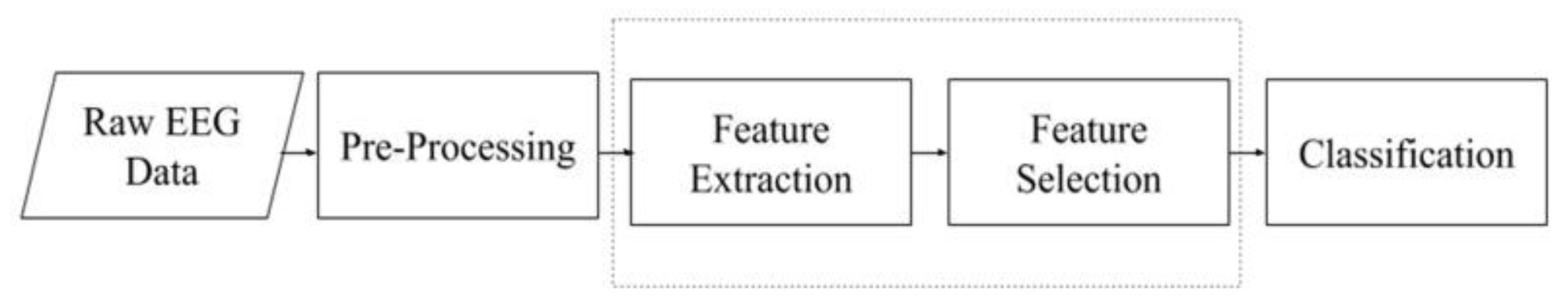
3. Methodology
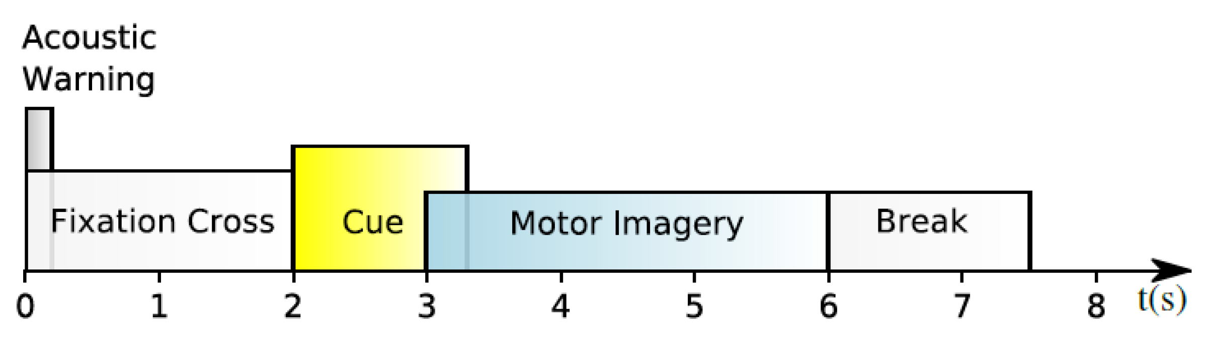
3.1. Data Preprocessing
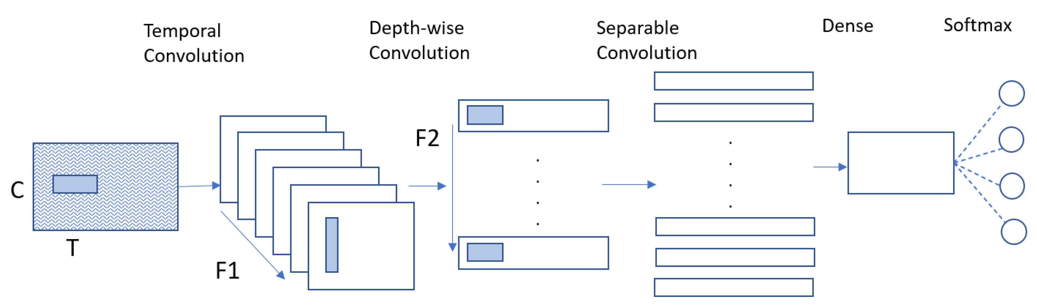
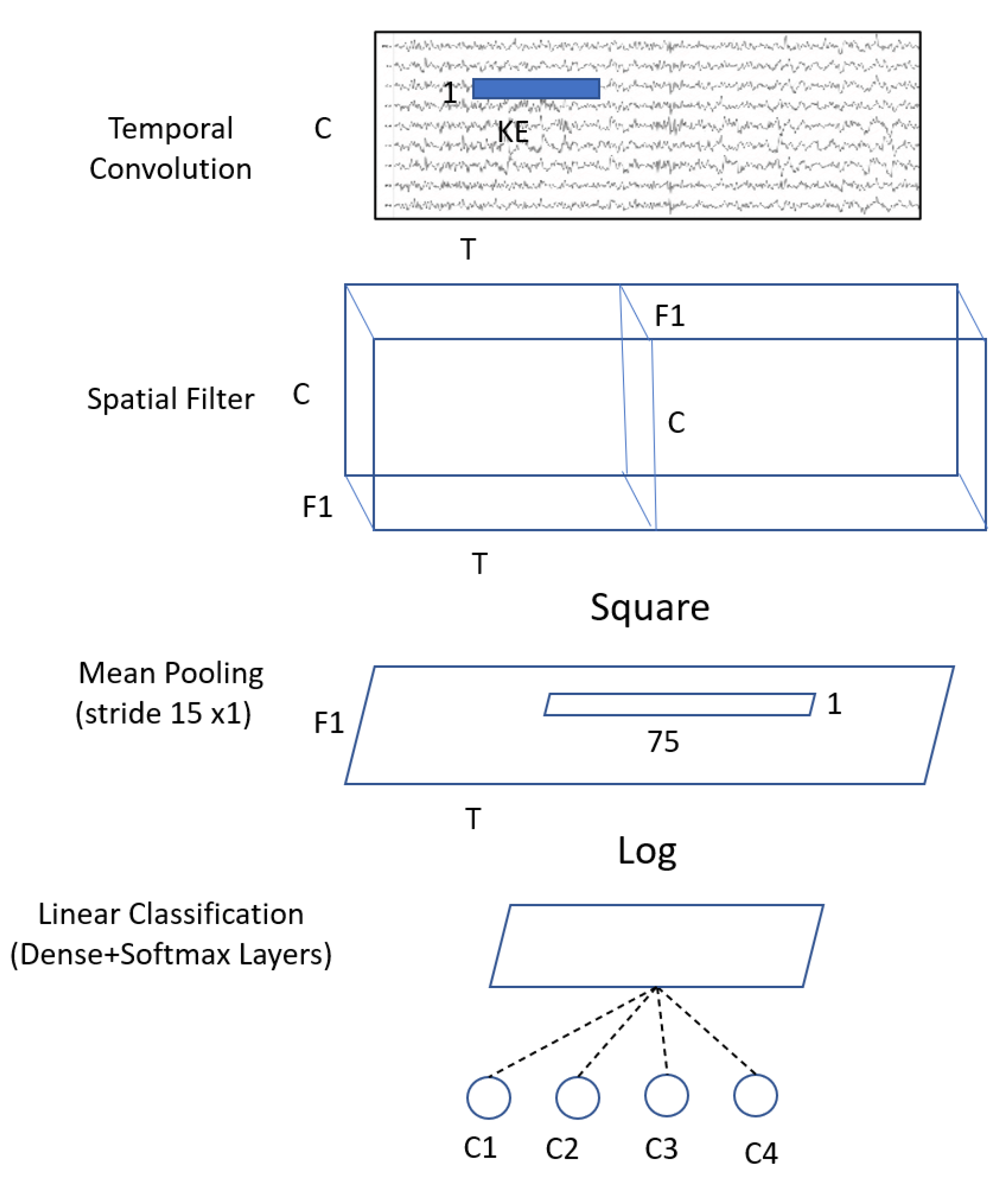
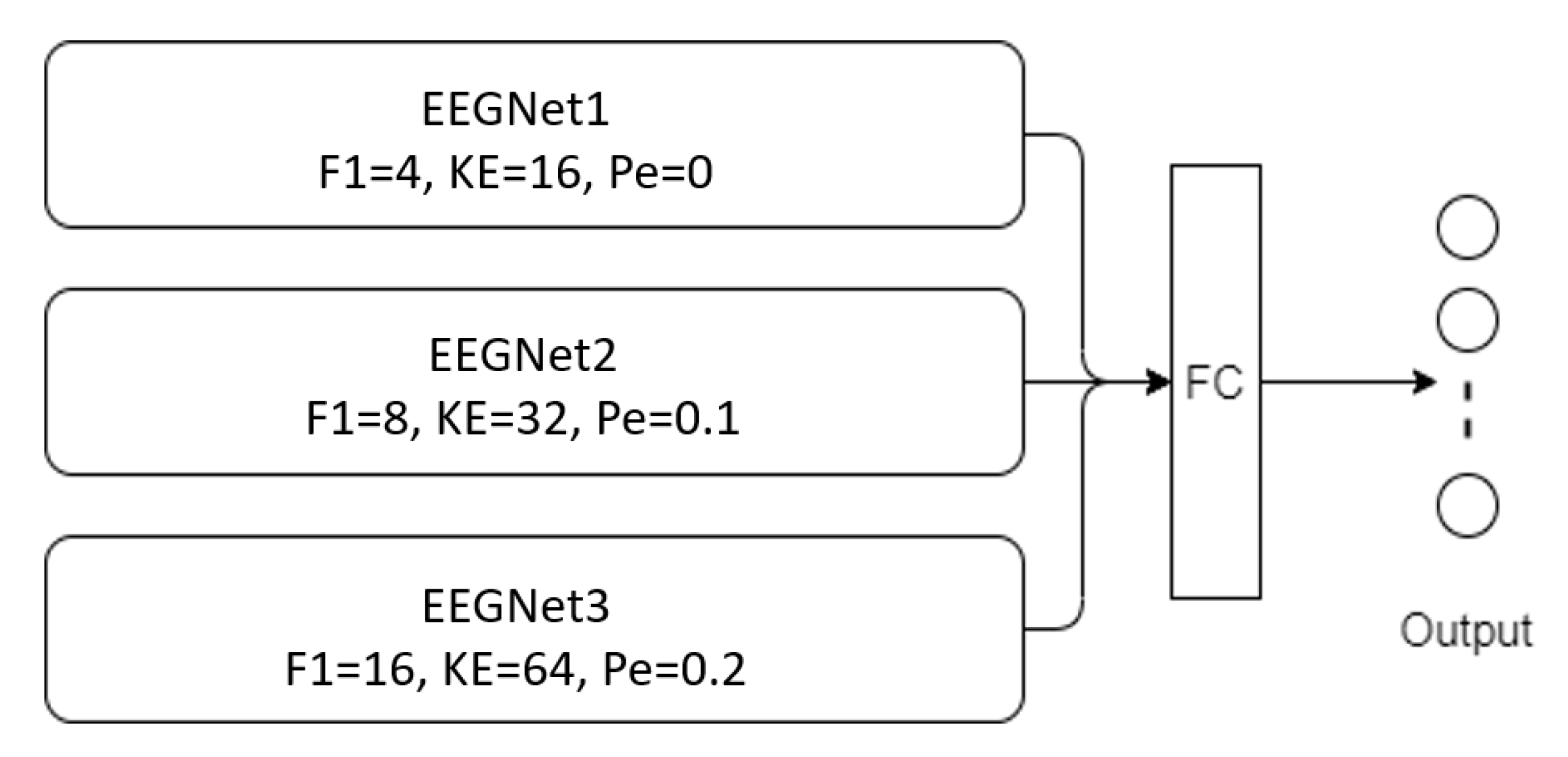
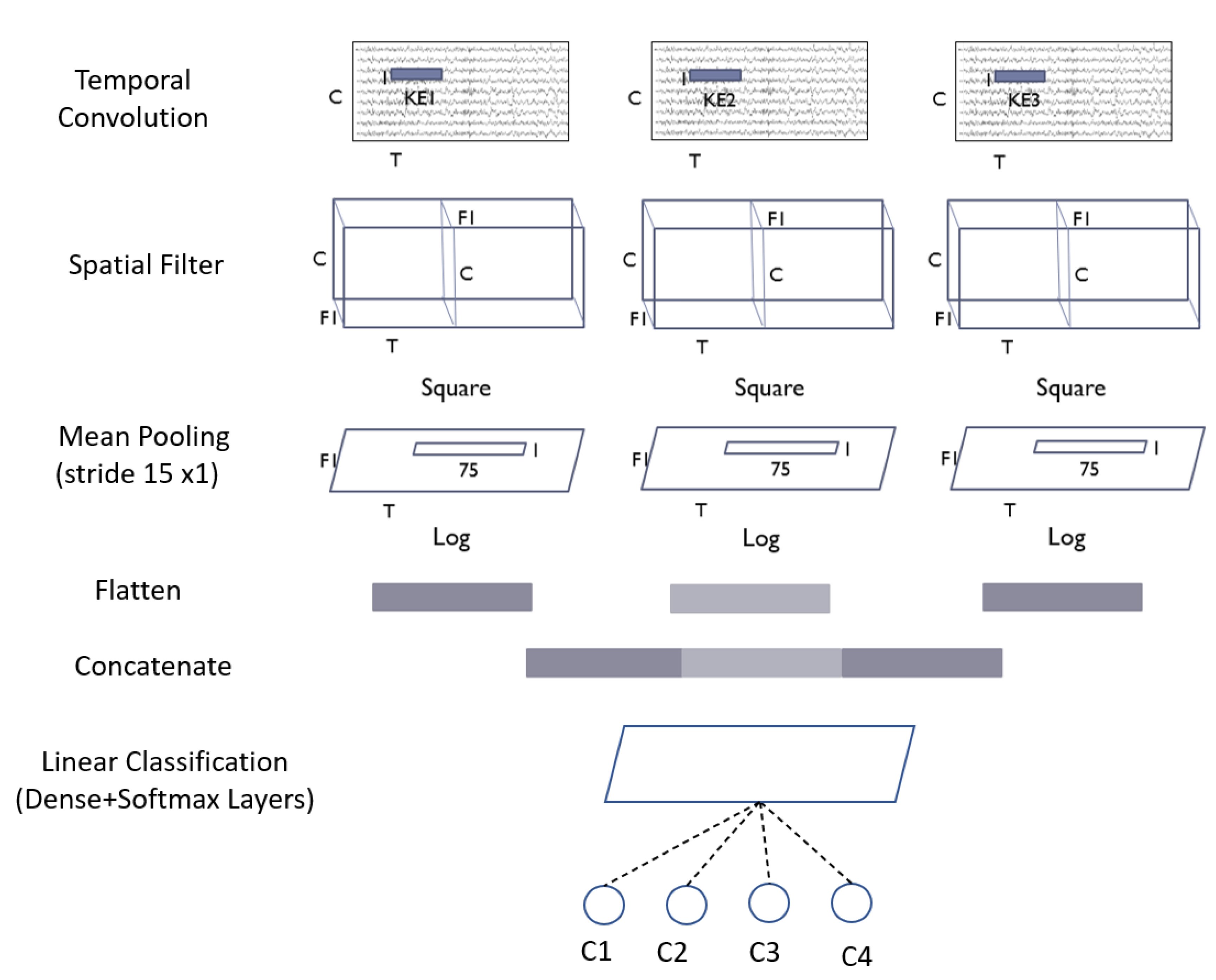
3.2. Proposed Models
3.3. Training Procedure
4. Experimental Results
4.1. Performance Metrics
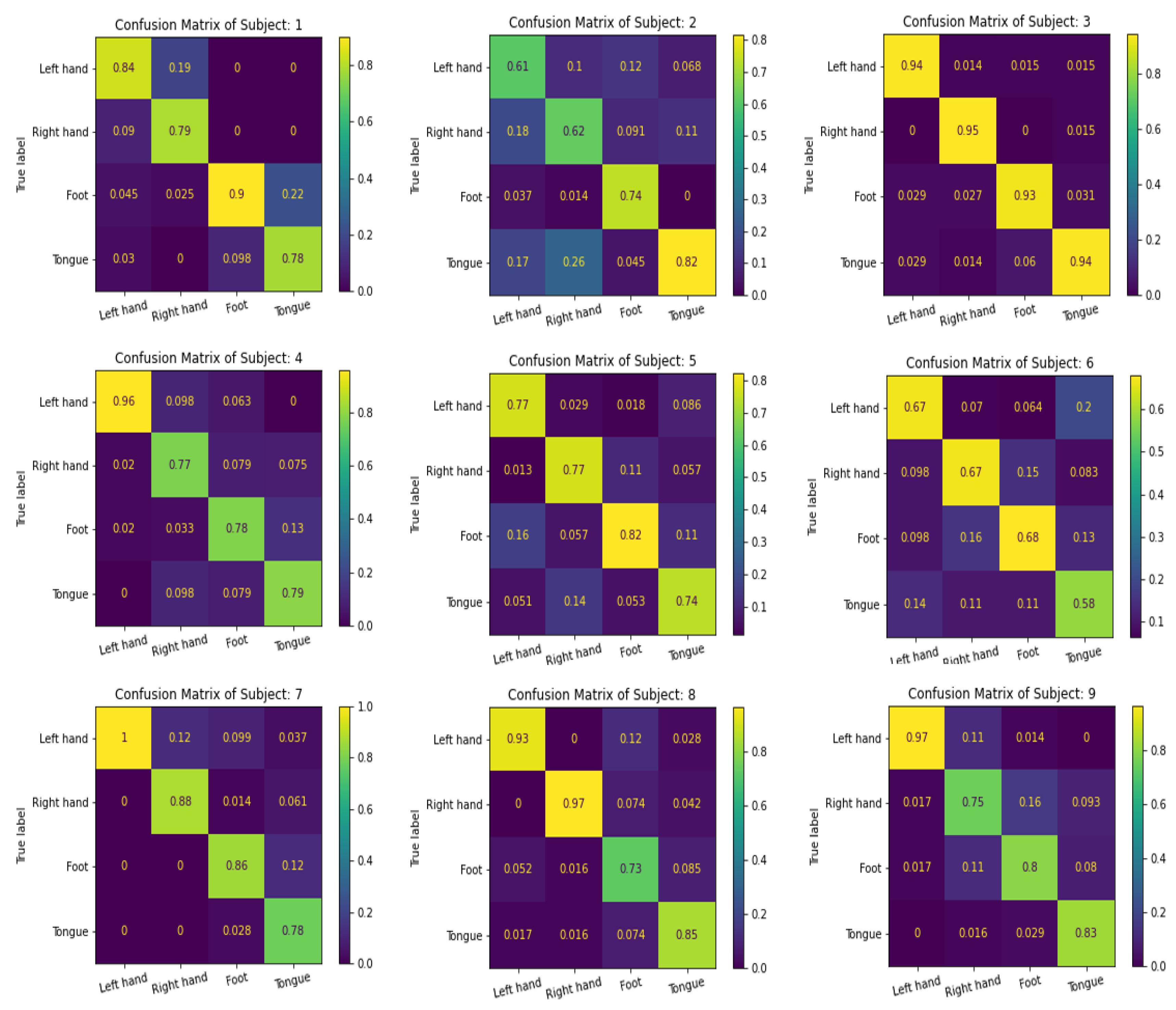
4.2. Results of BCI Competition IV-2a Dataset
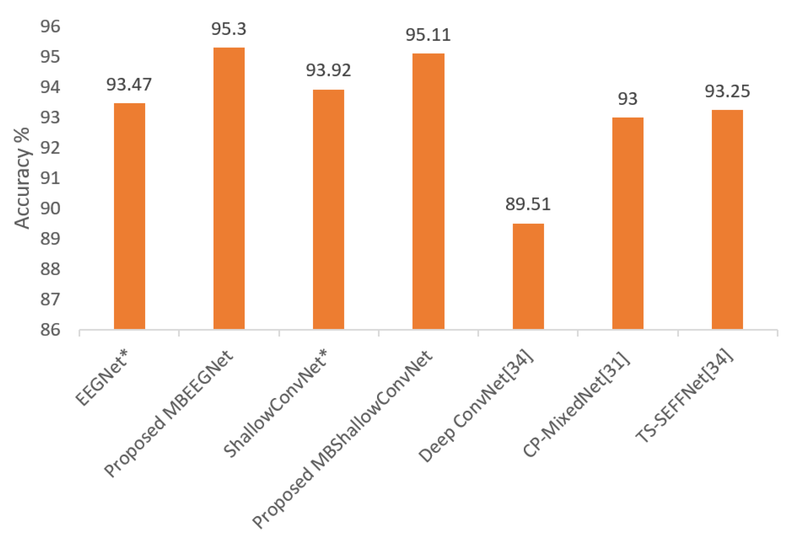
4.3. Results of HGD
5. Conclusions
Author Contributions
Funding
Institutional Review Board Statement
Informed Consent Statement
Data Availability Statement
Acknowledgments
Conflicts of Interest
References
- Muhammad, G.; Alshehri, F.; Karray, F.; El Saddik, A.; Alsulaiman, M.; Falk, T.H. A comprehensive survey on multimodal medical signals fusion for smart healthcare systems. Inf. Fusion 2021, 76, 355–375. [Google Scholar] [CrossRef]
- Alshehri, F.; Muhammad, G. A Comprehensive Survey of the Internet of Things (IoT) and AI-Based Smart Healthcare. IEEE Access 2020, 9, 3660–3678. [Google Scholar] [CrossRef]
- Musallam, Y.K.; AlFassam, N.I.; Muhammad, G.; Amin, S.U.; Alsulaiman, M.; Abdul, W.; Altaheri, H.; Bencherif, M.A.; Algabri, M. Electroencephalography-based motor imagery classification using temporal convolutional network fusion. Biomed. Signal Process. Control. 2021, 69, 102826. [Google Scholar] [CrossRef]
- Padfield, N.; Zabalza, J.; Zhao, H.; Masero, V.; Ren, J. EEG-Based Brain-Computer Interfaces Using Motor-Imagery: Techniques and Challenges. Sensors 2019, 19, 1423. [Google Scholar] [CrossRef] [Green Version]
- Caldwell, J.A.; Prazinko, B.; Caldwell, J. Body posture affects electroencephalographic activity and psychomotor vigilance task performance in sleep-deprived subjects. Clin. Neurophysiol. 2003, 114, 23–31. [Google Scholar] [CrossRef]
- Guideline Thirteen: Guidelines for Standard Electrode Position Nomenclature. J. Clin. Neurophysiol. 1994, 11, 111–113. [CrossRef]
- Altaheri, H.; Muhammad, G.; Alsulaiman, M.; Amin, S.U.; Altuwaijri, G.A.; Abdul, W.; Bencherif, M.A.; Faisal, M. Deep learning techniques for classification of electroencephalogram (EEG) motor imagery (MI) signals: A review. Neural Comput. Appl. 2021, 1–42. [Google Scholar] [CrossRef]
- Jung, R.; Berger, W. Hans Bergers Entdeckung des Elektrenkephalogramms und seine ersten Befunde 1924?1931. Eur. Arch. Psychiatry Clin. Neurosci. 1979, 227, 279–300. [Google Scholar] [CrossRef]
- Lotte, F.; Guan, C. Regularizing Common Spatial Patterns to Improve BCI Designs: Unified Theory and New Algorithms. IEEE Trans. Biomed. Eng. 2010, 58, 355–362. [Google Scholar] [CrossRef] [Green Version]
- Ang, K.K.; Chin, Z.Y.; Wang, C.; Guan, C.; Zhang, H. Filter Bank Common Spatial Pattern Algorithm on BCI Competition IV Datasets 2a and 2b. Front. Behav. Neurosci. 2012, 6, 39. [Google Scholar] [CrossRef] [Green Version]
- Elstob, D.; Secco, E.L. A Low Cost Eeg Based Bci Prosthetic Using Motor Imagery. Int. J. Inf. Technol. Converg. Serv. 2016, 6, 23–36. [Google Scholar] [CrossRef] [Green Version]
- Müller-Putz, G.R.; Ofner, P.; Schwarz, A.; Pereira, J.; Luzhnica, G.; di Sciascio, C.; Veas, E.; Stein, S.; Williamson, J.; Murray-Smith, R.; et al. Moregrasp: Restoration of Upper Limb Function in Individuals with High Spinal Cord Injury by Multimodal Neuroprostheses for Interaction in Daily Activities. In Proceedings of the 7th Graz Brain-Computer Interface Conference, Graz, Austria, 18 September 2017; pp. 338–343. [Google Scholar]
- Gomez-Rodriguez, M.; Grosse-Wentrup, M.; Hill, J.; Gharabaghi, A.; Scholkopf, B.; Peters, J. Towards brain-robot interfaces in stroke rehabilitation. In Proceedings of the 2011 IEEE International Conference on Rehabilitation Robotics, Zurich, Switzerland, 29 June–1 July 2011; Volume 2011, pp. 1–6. [Google Scholar]
- Al-Nasheri, A.; Muhammad, G.; Alsulaiman, M.; Ali, Z. Investigation of Voice Pathology Detection and Classification on Different Frequency Regions Using Correlation Functions. J. Voice 2017, 31, 3–15. [Google Scholar] [CrossRef]
- Wang, Z.; Yu, Y.; Xu, M.; Liu, Y.; Yin, E.; Zhou, Z. Towards a Hybrid BCI Gaming Paradigm Based on Motor Imagery and SSVEP. Int. J. Hum.-Comput. Interact. 2018, 35, 197–205. [Google Scholar] [CrossRef]
- Lawhern, V.J.; Solon, A.J.; Waytowich, N.R.; Gordon, S.M.; Hung, C.P.; Lance, B.J. EEGNet: A compact convolutional neural network for EEG-based brain–computer interfaces. J. Neural Eng. 2018, 15, 056013. [Google Scholar] [CrossRef] [PubMed] [Green Version]
- Schirrmeister, R.T.; Springenberg, J.T.; Fiederer, L.D.J.; Glasstetter, M.; Eggensperger, K.; Tangermann, M.; Hutter, F.; Burgard, W.; Ball, T. Deep learning with Convolutional Neural Networks for EEG decoding and visualization. Hum. Brain Mapp. 2017, 38, 5391–5420. [Google Scholar] [CrossRef] [PubMed] [Green Version]
- Bashivan, P.; Rish, I.; Yeasin, M.; Codella, N. Learning Representations from EEG with Deep Recurrent-Convolutional Neural Networks. arXiv 2015, arXiv:1511.06448v3. [Google Scholar]
- Tabar, Y.R.; Halici, U. A novel deep learning approach for classification of EEG motor imagery signals. J. Neural Eng. 2017, 14, 016003. [Google Scholar] [CrossRef] [PubMed]
- Tang, Z.; Li, C.; Sun, S. Single-trial EEG classification of motor imagery using deep Convolutional Neural Networks. Optik 2017, 130, 11–18. [Google Scholar] [CrossRef]
- Zhao, X.; Zhang, H.; Zhu, G.; You, F.; Kuang, S.; Sun, L. A Multi-Branch 3D Convolutional Neural Network for EEG-Based Motor Imagery Classification. IEEE Trans. Neural Syst. Rehabil. Eng. 2019, 27, 2164–2177. [Google Scholar] [CrossRef]
- Dose, H.; Møller, J.S.; Iversen, H.K.; Puthusserypady, S. An end-to-end deep learning approach to MI-EEG signal classification for BCIs. Expert Syst. Appl. 2018, 114, 532–542. [Google Scholar] [CrossRef]
- Sakhavi, S.; Guan, C.; Yan, S. Learning Temporal Information for Brain-Computer Interface Using Convolutional Neural Networks. IEEE Trans. Neural Netw. Learn. Syst. 2018, 29, 5619–5629. [Google Scholar] [CrossRef] [PubMed]
- Xu, B.; Zhang, L.; Song, A.; Wu, C.; Li, W.; Zhang, D.; Xu, G.; Li, H.; Zeng, H. Wavelet Transform Time-Frequency Image and Convolutional Network-Based Motor Imagery EEG Classification. IEEE Access 2018, 7, 6084–6093. [Google Scholar] [CrossRef]
- Amin, S.U.; Alsulaiman, M.; Muhammad, G.; Mekhtiche, M.A.; Hossain, M.S. Deep Learning for EEG motor imagery classification based on multi-layer CNNs feature fusion. Futur. Gener. Comput. Syst. 2019, 101, 542–554. [Google Scholar] [CrossRef]
- Zhou, H.; Zhao, X.; Zhang, H.; Kuang, S. The Mechanism of a Multi-Branch Structure for EEG-Based Motor Imagery Classification. In Proceedings of the 2019 IEEE International Conference on Robotics and Biomimetics (ROBIO), Dali, China, 6–8 December 2019; pp. 2473–2477. [Google Scholar]
- Jin, J.; Dundar, A.; Culurciello, E. Flattened Convolutional Neural Networks for feedforward acceleration. arXiv 2015, arXiv:1412.5474v4. [Google Scholar]
- Cecotti, H.; Graser, A. Convolutional Neural Networks for P300 Detection with Application to Brain-Computer Interfaces. IEEE Trans. Pattern Anal. Mach. Intell. 2011, 33, 433–445. [Google Scholar] [CrossRef]
- Riyad, M.; Khalil, M.; Adib, A. Incep-EEGNet: A ConvNet for Motor Imagery Decoding. In Proceedings of the 9th International Conference on Image and Signal Processing (ICISP), Marrakesh, Morocco, 4–6 June 2020; pp. 103–111. [Google Scholar]
- Ingolfsson, T.M.; Hersche, M.; Wang, X.; Kobayashi, N.; Cavigelli, L.; Benini, L. EEG-TCNet: An Accurate Temporal Convolutional Network for Embedded Motor-Imagery Brain–Machine Interfaces. In Proceedings of the 2020 IEEE International Conference on Systems, Man, and Cybernetics (SMC), Toronto, ON, Canada, 11–14 October 2020; pp. 2958–2965. [Google Scholar]
- Li, Y.; Zhang, X.-R.; Zhang, B.; Lei, M.-Y.; Cui, W.-G.; Guo, Y.-Z. A Channel-Projection Mixed-Scale Convolutional Neural Network for Motor Imagery EEG Decoding. IEEE Trans. Neural Syst. Rehabil. Eng. 2019, 27, 1170–1180. [Google Scholar] [CrossRef]
- Liu, X.; Shen, Y.; Liu, J.; Yang, J.; Xiong, P.; Lin, F. Parallel Spatial–Temporal Self-Attention CNN-Based Motor Imagery Classification for BCI. Front. Neurosci. 2020, 14, 587520. [Google Scholar] [CrossRef]
- Dai, G.; Zhou, J.; Huang, J.; Wang, N. HS-CNN: A CNN with hybrid convolution scale for EEG motor imagery classification. J. Neural Eng. 2019, 17, 016025. [Google Scholar] [CrossRef]
- Li, Y.; Guo, L.; Liu, Y.; Liu, J.; Meng, F. A Temporal-Spectral-Based Squeeze-and- Excitation Feature Fusion Network for Motor Imagery EEG Decoding. IEEE Trans. Neural Syst. Rehabil. Eng. 2021, 29, 1534–1545. [Google Scholar] [CrossRef]
- Brunner, C.; Leeb, R.; Muller-Putz, G.; Schlogl, A.; Pfurtscheller, G. BCI Competition 2008—Graz Data Set A; Institute for Knowledge Discovery (Laboratory of Brain-Computer Interfaces); Graz University of Technology: Graz, Austria, 2008; Volume 16, pp. 1–6. [Google Scholar]
- Roots, K.; Muhammad, Y.; Muhammad, N. Fusion Convolutional Neural Network for Cross-Subject EEG Motor Imagery Classification. Computers 2020, 9, 72. [Google Scholar] [CrossRef]
- Muhammad, G.; Hossain, M.S.; Kumar, N. EEG-Based Pathology Detection for Home Health Monitoring. IEEE J. Sel. Areas Commun. 2021, 39, 603–610. [Google Scholar] [CrossRef]
- Ioffe, S.; Szegedy, C. Batch Normalization: Accelerating Deep Network Training by Reducing Internal Covariate Shift. In Proceedings of the 32nd International Conference on Machine Learning, Lille, France, 6–11 July 2015; Volume 37, pp. 448–456. [Google Scholar]


| Related Work | Methods | Database | Acc% | Comment |
|---|---|---|---|---|
| Tang et al. [20] | 5-layer CNN | Private, with two subjects and two classes | 86.41% ± 0.77 | It is one of the first papers that used a deep learning model to classify EEG-based MI. The method was tested on a private database. |
| Dose et al. [22] | Shallow CNN | Physionet EEG Motor Movement/MI Dataset | 2classes 80.38% 3classes 69.8% 4classes 58.6% | As the number of classes increased, the accuracy dropped. |
| Sakhavi et al. [23] | FBCSP, C2CM | BCI competition IV-2a dataset | 74.46% (0.659 kappa) | The authors used the DL model as a classifier only after they extracted features using a handcrafted approach. |
| Xu et al. [24] | Wavelet transform time-frequency images, two-layer CNN | Dataset III from BCI competition II and dataset 2a from BCI competition IV | 92.75% 85.59% | This paper also used CNN as a classifier, and extracted the features from a combination of time-frequency images using wavelet transforms. |
| Zhao et al. [21] | Multi-branch 3D CNN | BCI competition IV-2a dataset | 75.02% (0.644 kappa) | The 3D filter has more complexity, which makes it difficult to implement in real-time applications. |
| Amin et al. [25] | Multi-layer CNN-based fusion models: MLP +CNN (MCNN) autoencoder + CNN (CCNN) | BCI competition IV-2a dataset and HGD | 75.7–95.4% 73.8–93.2% | Good accuracy using fixed parameters. |
| M. Riyad et al. [29] | Incep-EEGNet | BCI competition IV-2a | 74.07% | They preprocessed the data (resample the signals at 128 Hz, and filter with a bandpass filter between 1 Hz and 32 Hz); also used cropping as data augmentation, and they trained the model with different learning rates in a large number of epochs. |
| T. M. Ingolfsson et al. [30] | EEG-TCNET | BCI competition IV-2a | 77.35% | Good paper with good accuracy using fixed and variable parameters. |
| Y. Li et al. [31] | CP-MixedNet | BCI competition IV-2a dataset and HGD | 74.6% 93.7% | It is a good model that has a multiscale in a part of it, but has a large number of parameters (836 K). |
| X. Liu et al. [32] | Parallel spatial-temporal self-attention CNN | BCI competition IV-2a dataset and HGD | 78.51% 97.68% | A good paper that used self-attention in two parts. |
| Y. Li et al. [34] | TS-SEFFNet | BCI competition IV-2a dataset and HGD | 74.71% 93.25% | It is a big model that has a large number of parameters (282 K). |
| Branch | Hyperparameter | Value |
|---|---|---|
| First branch | Kernel size | 16 |
| Number of temporal filters | 4 | |
| Dropout rate | 0 | |
| Second branch | Kernel size | 32 |
| Number of temporal filters | 8 | |
| Dropout rate | 0.1 | |
| Third branch | Kernel size | 64 |
| Number of temporal filters | 16 | |
| Dropout rate | 0.2 |
| ←Subject | EEGNet [30] | EEG-TCNet [30] | Incep-EEGNet [29] | Variable EEGNet [30] | Our Proposed MBEEGNet | ShallowConvNet [30] | Our Proposed MBShallow CovNet | |||||||
|---|---|---|---|---|---|---|---|---|---|---|---|---|---|---|
| Acc. | κ | Acc. | κ | Acc. | κ | Acc. | κ | Acc. | κ | Acc. | κ | Acc. | κ | |
| S1 | 84.34 | 0.79 | 85.77 | 0.81 | 78.47 | 0.71 | 86.48 | 0.82 | 89.59 | 0.86 | 79.51 | 0.73 | 82.58 | 0.77 |
| S2 | 54.06 | 0.39 | 65.02 | 0.53 | 52.78 | 0.37 | 61.84 | 0.49 | 68.06 | 0.57 | 56.25 | 0.42 | 70.01 | 0.60 |
| S3 | 87.54 | 0.83 | 94.51 | 0.93 | 89.93 | 0.87 | 93.41 | 0.91 | 94.58 | 0.93 | 88.89 | 0.85 | 93.79 | 0.92 |
| S4 | 63.59 | 0.51 | 64.91 | 0.53 | 66.67 | 0.56 | 73.25 | 0.64 | 79.88 | 0.73 | 80.90 | 0.75 | 82.60 | 0.77 |
| S5 | 67.39 | 0.57 | 75.36 | 0.67 | 61.11 | 0.48 | 76.81 | 0.69 | 76.92 | 0.69 | 57.29 | 0.43 | 77.81 | 0.70 |
| S6 | 54.88 | 0.39 | 61.40 | 0.49 | 60.42 | 0.47 | 59.07 | 0.45 | 66.10 | 0.55 | 53.28 | 0.38 | 64.79 | 0.53 |
| S7 | 88.80 | 0.85 | 87.36 | 0.83 | 90.63 | 0.88 | 90.25 | 0.87 | 91.57 | 0.89 | 91.67 | 0.89 | 88.02 | 0.84 |
| S8 | 76.75 | 0.69 | 83.76 | 0.78 | 82.29 | 0.76 | 87.45 | 0.83 | 87.71 | 0.84 | 81.25 | 0.75 | 86.91 | 0.83 |
| S9 | 74.24 | 0.65 | 78.03 | 0.71 | 84.38 | 0.79 | 82.95 | 0.77 | 83.69 | 0.78 | 79.17 | 0.72 | 83.83 | 0.78 |
| Mean | 72.40 | 0.63 | 77.35 | 0.70 | 74.07 | 0.65 | 79.06 | 0.72 | 82.01 | 0.76 | 74.31 | 0.66 | 81.15 | 0.75 |
| S. D. | 13.27 | 0.18 | 11.57 | 0.15 | 14.06 | 0.19 | 12.28 | 0.16 | 10.13 | 0.13 | 14.54 | 0.19 | 9.04 | 0.12 |
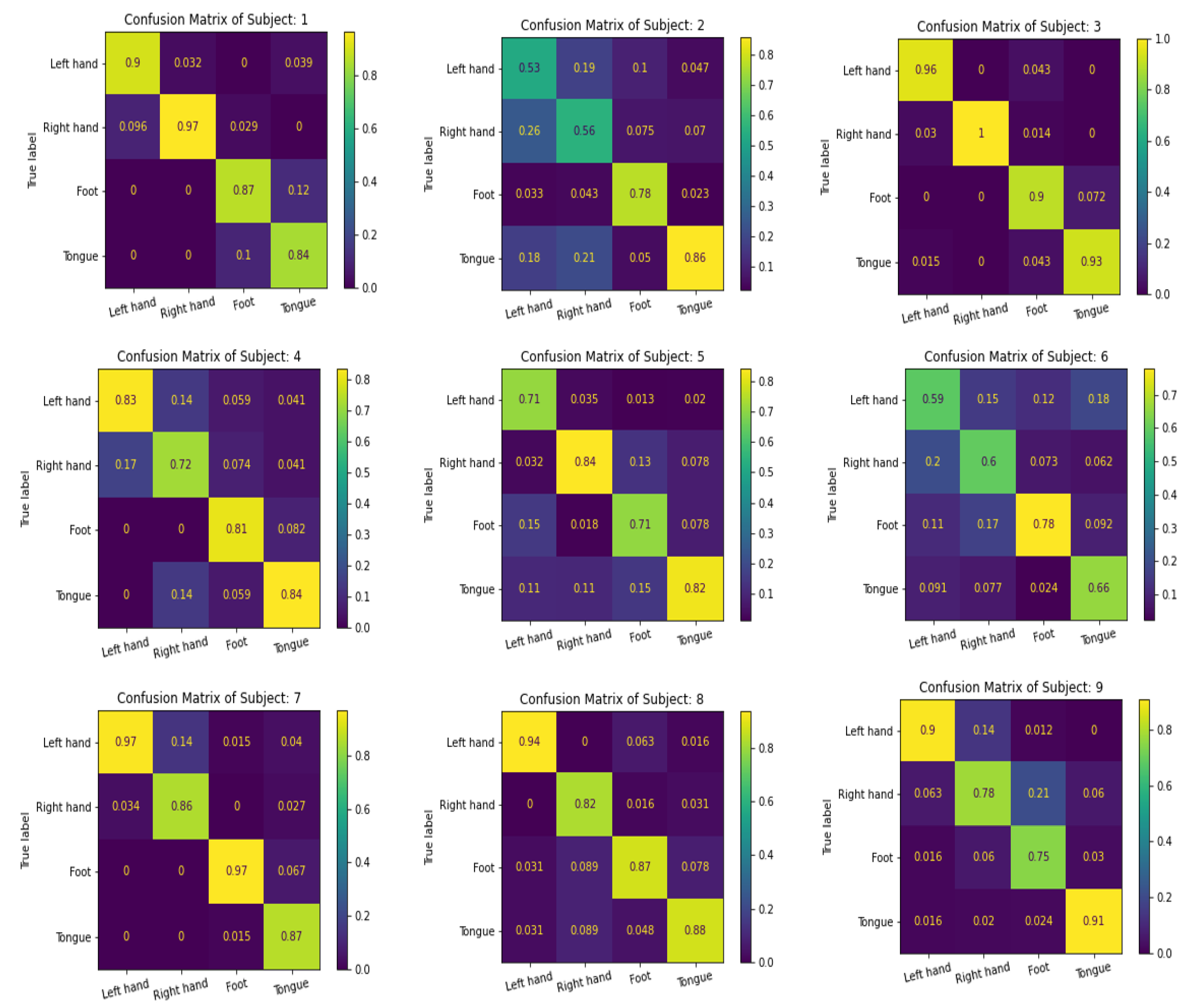
| 1 | 2 | 3 | 4 | 5 | 6 | 7 | 8 | 9 | Average | ||
|---|---|---|---|---|---|---|---|---|---|---|---|
| Precision | LH | 90.36 | 52.84 | 95.52 | 83.00 | 70.86 | 59.54 | 96.61 | 93.81 | 90.45 | 81.44 |
| RH | 96.81 | 55.83 | 100 | 72.00 | 83.75 | 60.18 | 86.00 | 82.16 | 78.00 | 79.41 | |
| F | 87.09 | 77.61 | 90.00 | 80.84 | 70.79 | 78.23 | 97.00 | 87.26 | 75.30 | 82.68 | |
| Tou. | 84.08 | 86.00 | 92.81 | 83.67 | 82.33 | 66.40 | 86.65 | 87.56 | 91.00 | 84.50 | |
| Avg. | 89.58 | 68.07 | 94.58 | 79.88 | 76.93 | 66.09 | 91.57 | 87.70 | 83.69 | 82.01 | |
| Recall | LH | 92.69 | 61.13 | 95.71 | 77.57 | 91.26 | 56.73 | 83.26 | 92.25 | 85.55 | 81.79 |
| RH | 88.58 | 58.03 | 95.78 | 71.64 | 77.78 | 64.17 | 93.38 | 94.58 | 70.08 | 79.34 | |
| F | 87.88 | 88.74 | 92.59 | 90.81 | 74.27 | 67.71 | 93.54 | 81.46 | 87.62 | 84.96 | |
| Tou. | 89.36 | 66.15 | 94.13 | 80.85 | 68.91 | 77.46 | 98.30 | 83.97 | 93.81 | 83.66 | |
| Avg. | 89.63 | 68.51 | 94.55 | 80.22 | 78.05 | 66.52 | 92.12 | 88.06 | 84.27 | 82.44 | |
| F1 Score | Avg. | 89.61 | 68.29 | 94.57 | 80.05 | 77.49 | 66.30 | 91.84 | 87.88 | 83.98 | 82.22 |
| 1 | 2 | 3 | 4 | 5 | 6 | 7 | 8 | 9 | AVG. | ||
|---|---|---|---|---|---|---|---|---|---|---|---|
| Precision | LH | 83.58 | 61.18 | 94.19 | 96.00 | 77.46 | 66.60 | 100 | 93.09 | 96.61 | 85.41 |
| RH | 78.61 | 62.37 | 94.53 | 77.08 | 77.31 | 66.34 | 88.00 | 96.81 | 76.06 | 79.68 | |
| F | 90.18 | 74.30 | 92.54 | 77.92 | 81.92 | 67.73 | 85.91 | 73.15 | 79.76 | 80.39 | |
| Tou. | 78.00 | 82.16 | 93.91 | 79.40 | 74.52 | 58.41 | 78.16 | 84.58 | 82.75 | 79.10 | |
| Avg. | 82.59 | 70.00 | 93.79 | 82.60 | 77.80 | 64.77 | 88.02 | 86.91 | 83.80 | 81.14 | |
| Recall | LH | 81.55 | 67.93 | 95.53 | 85.64 | 85.27 | 66.73 | 79.62 | 86.27 | 88.66 | 81.91 |
| RH | 89.77 | 61.94 | 98.45 | 81.57 | 81.05 | 66.93 | 92.15 | 89.32 | 73.53 | 81.63 | |
| F | 75.63 | 93.55 | 91.44 | 81.00 | 71.49 | 63.67 | 87.75 | 82.67 | 79.44 | 80.74 | |
| Tou. | 85.90 | 63.32 | 90.12 | 81.70 | 75.20 | 61.70 | 96.53 | 88.82 | 94.86 | 82.02 | |
| Avg. | 83.21 | 71.68 | 93.89 | 82.47 | 78.25 | 64.76 | 89.01 | 86.77 | 84.12 | 81.58 | |
| F1 Score | Avg. | 82.90 | 70.83 | 93.84 | 82.54 | 78.03 | 64.76 | 88.51 | 86.84 | 83.96 | 81.36 |
| Methods | Hyperparameters | Activation Function | Average Accuracy (%) |
|---|---|---|---|
| MBEEGNet | B1:F1 = 8, KE = 32, Pe = 0.2 B2:F1 = 16, KE = 64, Pe = 0.1 B3:F1 = 32, KE = 128, Pe = 0 | Relu | 77.03 |
| B1:F1 = 8, KE = 32, Pe = 0.2 B2:F1 = 16, KE = 64, Pe = 0.1 B3:F1 = 32, KE = 128, Pe = 0 | elu | 80.30 | |
| B1:F1 = 4, KE = 16, Pe = 0 B2:F1 = 8, KE = 32, Pe = 0.1 B3:F1 = 16, KE = 64, Pe = 0.2 | Relu | 78.63 | |
| B1:F1 = 4, KE = 16, Pe = 0 B2:F1 = 8, KE = 32, Pe = 0.1 B3:F1 = 16, KE = 64, Pe = 0.2 | elu | 82.01 | |
| MBShallowConvNet | KE1 = 10, KE2 = 20, KE3 = 30 | - | 80.36 |
| KE1 = 15, KE2 = 25, KE3 = 35 | - | 78.63 | |
| KE1 = 5, KE2 = 15, KE3 = 20 | - | 81.15 |
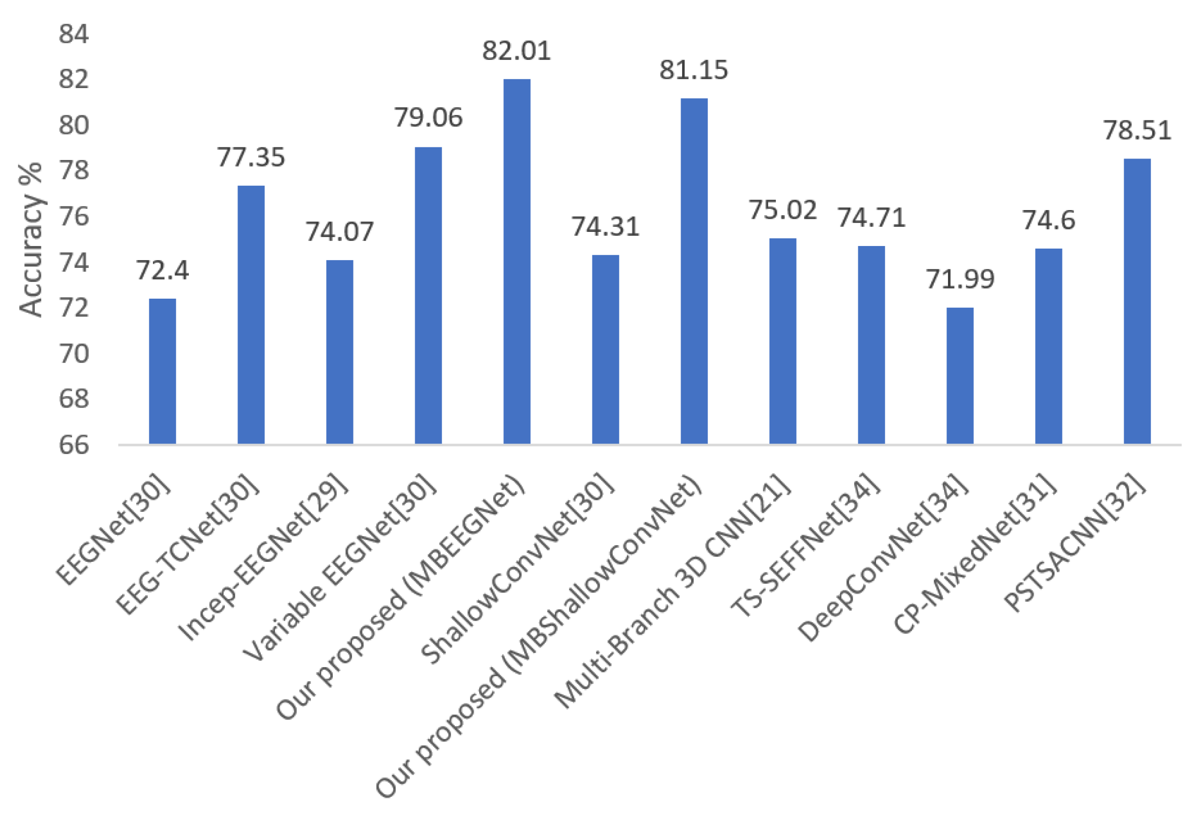
| Methods | Mean Accuracy (%) | Number of Parameters |
|---|---|---|
| DeepConvNet [32] | 71.99 | 284 × 103 |
| EEGNet [29] | 72.40 | 2.63 × 10³ |
| ShallowConvNet [29] | 74.31 | 47.31 × 10³ |
| TS-SEFFNet [32] | 74.71 | 282 × 103 |
| CP-MixedNet [32] | 74.60 | 836 × 103 |
| EEG-TCNet [29] | 77.35 | 4.27 × 10³ |
| Variable EEGNet [29] | 79.06 | 15.6 × 10³ |
| Our proposed (MBEEGNet) | 82.01 | 8.908 × 10³ |
| Our proposed (MBShallowConvNet) | 81.15 | 147.22 × 10³ |
| Methods/Subj. | 1 | 2 | 3 | 4 | 5 | 6 | 7 | 8 | 9 | 10 | 11 | 12 | 13 | 14 | Mean | Std. Dev. |
|---|---|---|---|---|---|---|---|---|---|---|---|---|---|---|---|---|
| EEGNet * | 94.37 | 92.50 | 100 | 96.25 | 96.87 | 98.12 | 93.07 | 96.87 | 98.12 | 91.25 | 80.00 | 96.25 | 95.60 | 79.37 | 93.47 | 6.30 |
| MBEEGNet | 95.02 | 95.02 | 100 | 99.40 | 98.17 | 98.80 | 93.13 | 95.52 | 98.18 | 92.14 | 89.43 | 96.02 | 94.45 | 88.88 | 95.30 | 3.50 |
| ShallowConvNet * | 96.87 | 93.75 | 99.37 | 98.12 | 98.12 | 93.12 | 92.45 | 96.87 | 98.12 | 90.62 | 76.25 | 95.00 | 94.96 | 91.25 | 93.92 | 5.79 |
| MBShallowConvNet | 98.25 | 96.23 | 98.80 | 98.18 | 97.65 | 96.90 | 93.80 | 97.00 | 97.52 | 92.50 | 80.78 | 96.25 | 95.62 | 92.04 | 95.11 | 4.62 |
| DeepConvNet [34] | 81.88 | 91.88 | 93.13 | 92.50 | 90.63 | 93.13 | 84.28 | 90.80 | 96.88 | 85.00 | 88.13 | 91.25 | 89.94 | 83.75 | 89.51 | 4.32 |
| TS-SEFFNet [34] | 90.69 | 93.53 | 98.53 | 96.88 | 92.90 | 93.53 | 92.40 | 91.78 | 96.88 | 89.88 | 92.78 | 95.40 | 93.03 | 87.34 | 93.25 | 2.97 |
| 1 | 2 | 3 | 4 | 5 | 6 | 7 | 8 | 9 | 10 | 11 | 12 | 13 | 14 | AVG. | ||
|---|---|---|---|---|---|---|---|---|---|---|---|---|---|---|---|---|
| Precision | LH | 92.81 | 95.19 | 100 | 100 | 95.19 | 97.61 | 92.54 | 97.10 | 97.61 | 95.00 | 79.56 | 100 | 92.09 | 84.34 | 94.22 |
| RH | 94.81 | 97.49 | 100 | 100 | 100 | 100 | 90.27 | 85.00 | 95.10 | 93.00 | 88.56 | 100 | 88.09 | 83.08 | 93.96 | |
| F | 97.39 | 94.72 | 100 | 100 | 97.49 | 100 | 95.00 | 100 | 100 | 93.91 | 95.19 | 87.00 | 100 | 88.09 | 96.34 | |
| Tou. | 95.10 | 92.72 | 100 | 97.61 | 100 | 97.61 | 94.71 | 100 | 100 | 86.61 | 94.38 | 97.10 | 97.61 | 100 | 96.67 | |
| Avg. | 95.03 | 95.03 | 100 | 99.40 | 98.17 | 98.80 | 93.13 | 95.52 | 98.18 | 92.13 | 89.42 | 96.02 | 94.45 | 88.88 | 95.30 | |
| Recall | LH | 97.28 | 97.44 | 100 | 100 | 100 | 100 | 92.72 | 86.61 | 100 | 95.38 | 93.71 | 100 | 90.64 | 81.47 | 95.38 |
| RH | 92.77 | 97.59 | 100 | 100 | 97.66 | 97.66 | 94.74 | 96.70 | 97.54 | 100 | 81.65 | 100 | 91.76 | 84.35 | 95.17 | |
| F | 93.00 | 90.73 | 100 | 97.66 | 97.58 | 97.66 | 94.72 | 100 | 95.33 | 81.95 | 97.04 | 96.77 | 95.42 | 92.15 | 95.00 | |
| Tou. | 97.34 | 94.61 | 100 | 100 | 97.56 | 100 | 90.56 | 100 | 100 | 93.38 | 87.04 | 88.18 | 100 | 97.66 | 96.17 | |
| Avg. | 95.10 | 95.09 | 100 | 99.41 | 98.20 | 98.83 | 93.18 | 95.83 | 98.22 | 92.68 | 89.86 | 96.24 | 94.46 | 88.91 | 95.43 | |
| F1 Score | Avg. | 95.06 | 95.06 | 100 | 99.41 | 98.18 | 98.82 | 93.16 | 95.68 | 98.20 | 92.40 | 89.64 | 96.13 | 94.45 | 88.89 | 95.36 |
| κ-Score | Avg. | 93.37 | 93.36 | 100 | 99.40 | 97.56 | 98.40 | 90.84 | 94.03 | 97.57 | 89.52 | 85.90 | 94.70 | 92.60 | 85.18 | 93.73 |
| 1 | 2 | 3 | 4 | 5 | 6 | 7 | 8 | 9 | 10 | 11 | 12 | 13 | 14 | AVG. | ||
|---|---|---|---|---|---|---|---|---|---|---|---|---|---|---|---|---|
| Precision | LH | 100 | 97.61 | 100 | 97.61 | 93.09 | 97.39 | 86.00 | 97.29 | 95.19 | 92.81 | 73.15 | 97.39 | 97.39 | 91.91 | 94.06 |
| RH | 93.00 | 97.39 | 100 | 97.49 | 100 | 100 | 94.28 | 90.73 | 97.49 | 92.72 | 65.59 | 97.61 | 92.54 | 83.75 | 93.04 | |
| F | 100 | 94.81 | 100 | 100 | 100 | 95 | 97.49 | 100 | 97.39 | 91.91 | 90.27 | 95.00 | 97.39 | 92.54 | 96.56 | |
| Tou. | 100 | 95.10 | 95.19 | 97.61 | 97.49 | 95.19 | 97.49 | 100 | 100 | 92.54 | 94.00 | 95.00 | 95.19 | 100 | 96.77 | |
| Avg. | 98.25 | 96.23 | 98.80 | 98.18 | 97.65 | 96.90 | 93.81 | 97.00 | 97.52 | 92.50 | 80.75 | 96.25 | 95.63 | 92.05 | 95.11 | |
| Recall | LH | 97.75 | 100 | 100 | 100 | 100 | 95.10 | 93.78 | 91.25 | 100 | 97.48 | 72.35 | 95.19 | 95.10 | 86.55 | 94.61 |
| RH | 100 | 95.10 | 100 | 97.59 | 97.75 | 97.47 | 87.04 | 97.12 | 97.59 | 95.09 | 75.23 | 100 | 92.45 | 88.79 | 94.37 | |
| F | 100 | 92.68 | 95.42 | 95.33 | 95.42 | 95.19 | 97.49 | 100 | 95.19 | 86.14 | 92.98 | 94.91 | 95.19 | 93 | 94.92 | |
| Tou. | 95.51 | 97.34 | 100 | 100 | 97.68 | 100 | 97.49 | 100 | 97.47 | 91.99 | 82.10 | 95.00 | 100 | 100 | 96.75 | |
| Avg. | 98.32 | 96.28 | 98.85 | 98.23 | 97.71 | 96.94 | 93.95 | 97.09 | 97.56 | 92.68 | 80.66 | 96.27 | 95.68 | 92.09 | 95.17 | |
| F1 Score | Avg. | 98.28 | 96.25 | 98.83 | 98.20 | 97.68 | 96.92 | 93.88 | 97.05 | 97.54 | 92.59 | 80.71 | 96.26 | 95.66 | 92.07 | 95.14 |
| κ-Score | Avg. | 97.67 | 94.97 | 98.40 | 97.57 | 96.86 | 95.86 | 91.74 | 96.00 | 96.69 | 89.99 | 74.37 | 95.00 | 94.16 | 89.39 | 93.48 |
Publisher’s Note: MDPI stays neutral with regard to jurisdictional claims in published maps and institutional affiliations. |
© 2022 by the authors. Licensee MDPI, Basel, Switzerland. This article is an open access article distributed under the terms and conditions of the Creative Commons Attribution (CC BY) license (https://creativecommons.org/licenses/by/4.0/).
Share and Cite
Altuwaijri, G.A.; Muhammad, G. A Multibranch of Convolutional Neural Network Models for Electroencephalogram-Based Motor Imagery Classification. Biosensors 2022, 12, 22. https://doi.org/10.3390/bios12010022
Altuwaijri GA, Muhammad G. A Multibranch of Convolutional Neural Network Models for Electroencephalogram-Based Motor Imagery Classification. Biosensors. 2022; 12(1):22. https://doi.org/10.3390/bios12010022
Chicago/Turabian StyleAltuwaijri, Ghadir Ali, and Ghulam Muhammad. 2022. "A Multibranch of Convolutional Neural Network Models for Electroencephalogram-Based Motor Imagery Classification" Biosensors 12, no. 1: 22. https://doi.org/10.3390/bios12010022
APA StyleAltuwaijri, G. A., & Muhammad, G. (2022). A Multibranch of Convolutional Neural Network Models for Electroencephalogram-Based Motor Imagery Classification. Biosensors, 12(1), 22. https://doi.org/10.3390/bios12010022