

FeCo: Hysteresis, Pseudo-Critical, and Compensation Temperatures on Quasi-Spherical Nanoparticle


Abstract
1. Introduction
2. Model and Computational Method
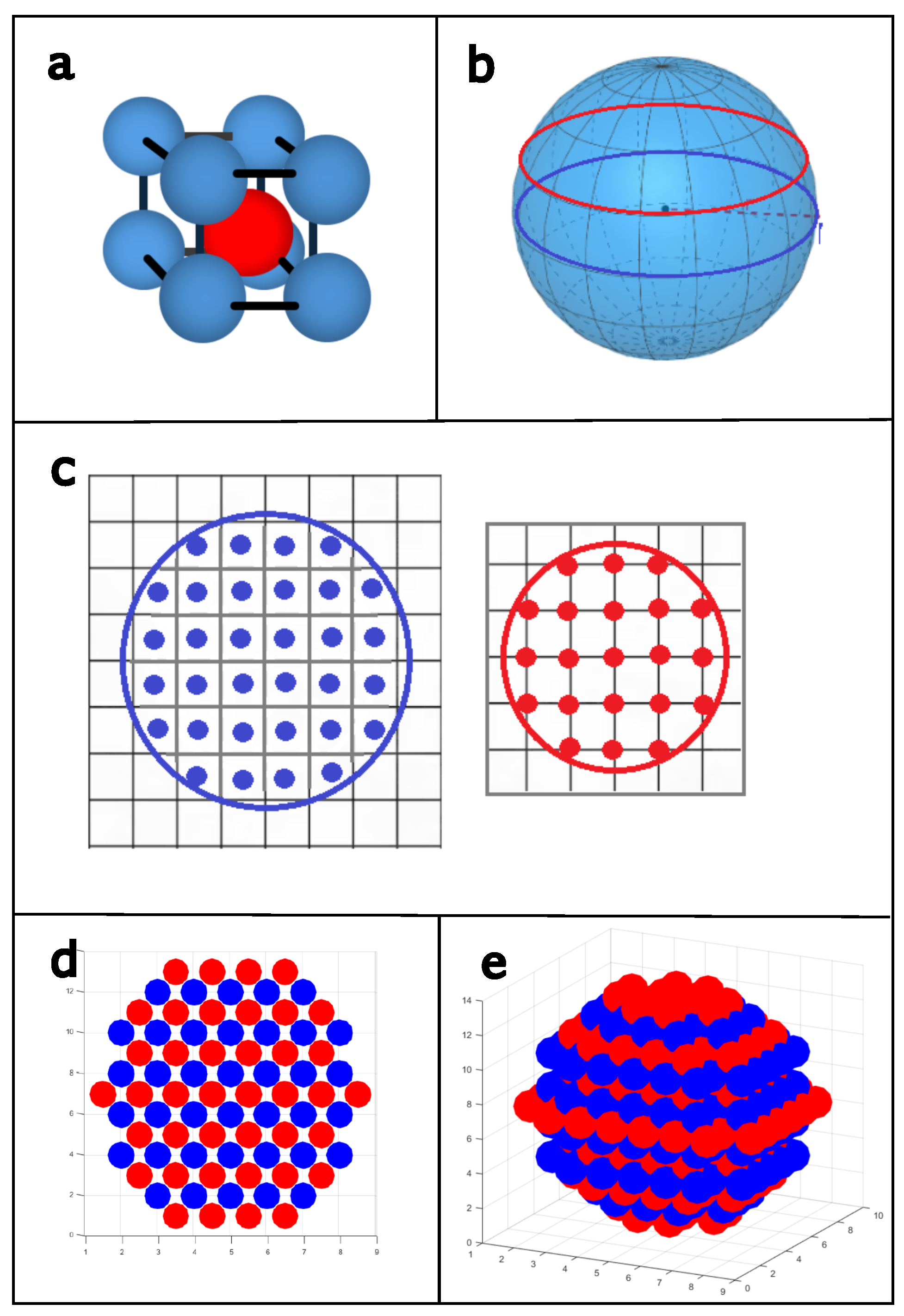
2.1. Model
2.2. Monte Carlo Simulations
3. Results
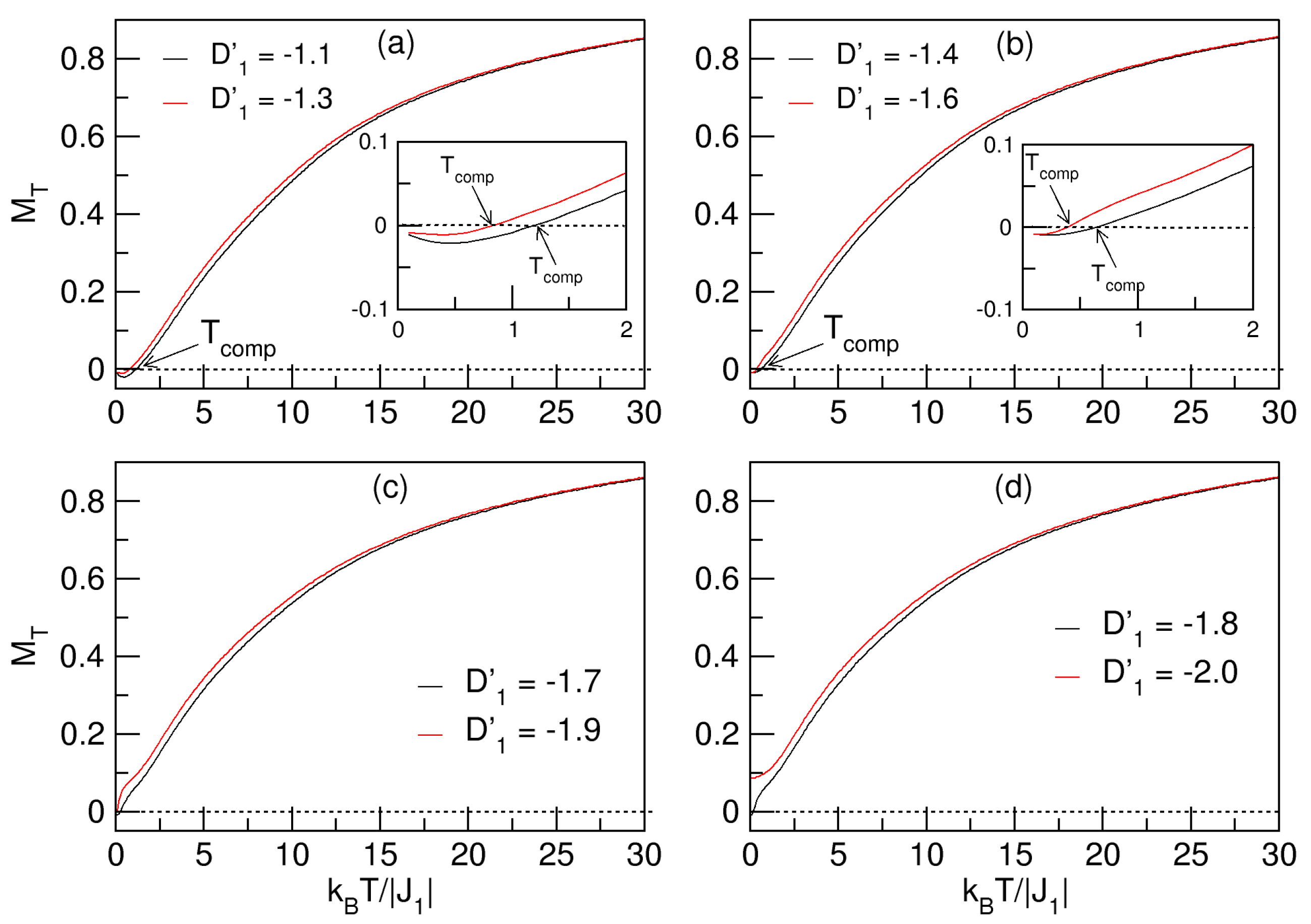
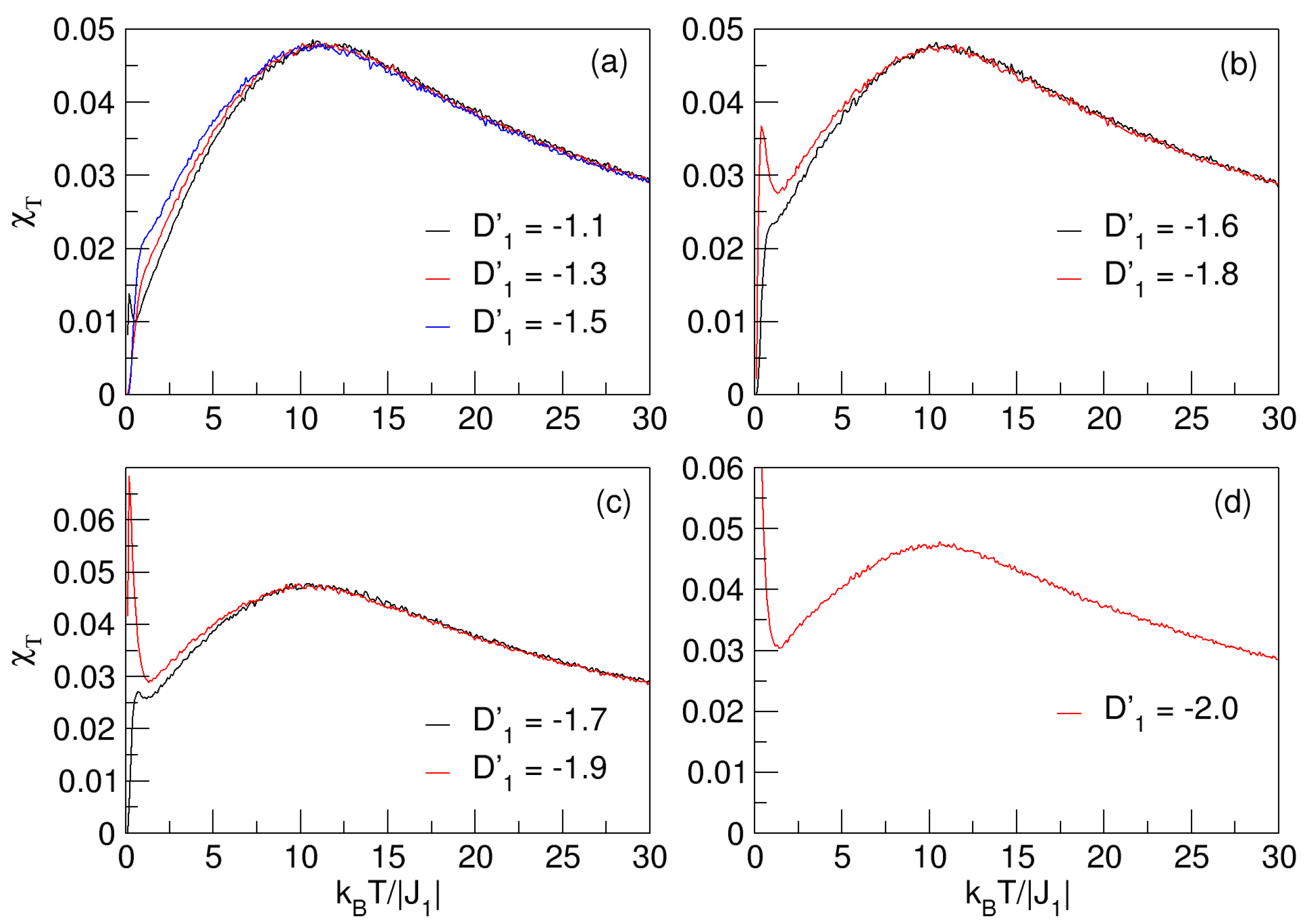
3.1. –– Model: Effects of
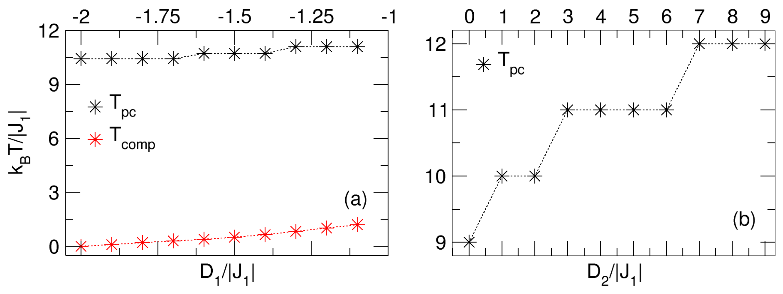
3.2. –– Model: Effects of
3.3. –– Model: Effects of
3.4. Hysteresis Behavior at Different Temperatures
3.4.1. Influences of Anisotropy:
3.4.2. Influences of Anisotropy:
3.4.3. Influences of Anisotropy:
4. Discussion
Author Contributions
Funding
Data Availability Statement
Acknowledgments
Conflicts of Interest
References
- Vatansever, E. Monte Carlo simulation of dynamic phase transitions and frequency dispersions of hysteresis curves in core/shell ferrimagnetic cubic nanoparticle. Phys. Lett. A 2017, 381, 1535–1542. [Google Scholar] [CrossRef]
- Saber, N.; Fadil, Z.; Mhirech, A.; Kabouchi, B.; Bahmad, L.; Ousi, B.W. Magnetic properties of the ternary FeCoxNi1−x alloy: Monte Carlo simulations. Philos. Mag. 2022, 102, 1725–1738. [Google Scholar] [CrossRef]
- Kima, K.J.; Leeb, S.J.; Lynch, D.W. Study of optical properties and electronic structure of ferromagnetic FeCo. Solid State Commun. 2000, 114, 457–460. [Google Scholar] [CrossRef]
- Lucas, M.S.; Muñoz, J.A.; Mauger, L.; Chen, W.L.; Sheets, A.O.; Turgut, Z.; Horwath, J.; Abernathy, D.L.; Stone, M.B.; Delaire, O.; et al. Effects of chemical composition and B2 order on phonons in bcc Fe-Co alloys. J. Appl. Phys. 2010, 108, 023519. [Google Scholar] [CrossRef]
- Sundar, R.S.; Deevi, S.C. Soft magnetic FeCo alloys: Alloy development, processing, and properties. Int. Mater. Rev. 2005, 50, 157–192. [Google Scholar] [CrossRef]
- Seo, W.S.; Lee, J.H.; Sun, X.; Suzuki, Y.; Mann, D.; Liu, Z.; Terashima, M.; Yang, P.C.; McConnell, M.V.; Nishimura, D.G.; et al. FeCo/graphitic-shell nanocrystals as advanced magnetic-resonance-imaging and near-infrared agents. Nat. Mater. 2006, 5, 971–976. [Google Scholar] [CrossRef] [PubMed]
- Moores, B.A.; Eichler, A.; Tao, Y.; Takahashi, H.; Navaretti, P.; Degen, C.L. Accelerated nanoscale magnetic resonance imaging through phase multiplexing. Appl. Phys. Lett. 2015, 106, 213101. [Google Scholar] [CrossRef]
- Hütten, A.; Sudfeld, D.; Ennen, I.; Reiss, G.; Hachmann, W.; Heinzmann, U.; Wojczykowski, K.; Jutzi, P.; Saikaly, W.; Thomas, G. New magnetic nanoparticles for biotechnology. J. Biotechnol. 2004, 112, 47–63. [Google Scholar] [CrossRef] [PubMed]
- Mehdaoui, B.; Carrey, J.; Stadler, M.; Cornejo, A.; Nayral, C.; Delpech, F.; Chaudret, B.; Respaud, M. Influence of a transverse static magnetic field on the magnetic hyperthermia properties and high-frequency hysteresis loops of ferromagnetic FeCo nanoparticles. Appl. Phys. Lett. 2012, 100, 052403. [Google Scholar] [CrossRef]
- Snyder, R.L.; Nguyen, V.Q.; Ramanujan, R.V. Design parameters for magneto-elastic soft actuators. Smart Mater. Struct. 2010, 19, 055017. [Google Scholar] [CrossRef]
- Ahmed, A.S.; Ramanujan, R.V. Hysteretic Buckling for Actuation of Magnet–Polymer Composites. Macromol. Chem. Phys. 2015, 216, 1594–1602. [Google Scholar] [CrossRef]
- Tang, Y.J.; Parker, F.T.; Harper, H.; Berkowitz, A.E.; Jiang, Q.; Smith, D.J.; Brand, M.; Wang, F. Co/sub 50/Fe/sub 50/ fine particles for power frequency applications. IEEE Trans. Magn. 2004, 40, 2002–2004. [Google Scholar] [CrossRef]
- Li, D.; Wang, Z.; Han, X.; Li, Y.; Guo, X.; Zuo, Y.; Xi, L. Improved high-frequency soft magnetic properties of FeCo films on organic ferroelectric PVDF substrate. J. Magn. Magn. Mater. 2015, 375, 33–37. [Google Scholar] [CrossRef]
- Lv, R.; Kang, F.; Gu, J.; Gui, X.; Wei, J.; Wang, K.; Wu, D. Carbon nanotubes filled with ferromagnetic alloy nanowires: Lightweight and wideband microwave absorber. Appl. Phys. Lett. 2008, 93, 223105. [Google Scholar] [CrossRef]
- Zhang, Y.; Wang, P.; Wang, Y.; Qiao, L.; Wang, T.; Li, F. Synthesis and excellent electromagnetic wave absorption properties of parallel aligned FeCo@C core–shell nanoflake composites. J. Mater. Chem. C 2015, 3, 10813–10818. [Google Scholar] [CrossRef]
- Bian, B.; Jin, L.; Zheng, Q.; Wang, F.; Xu, X.; Du, J. Exchange-coupled nanocomposites with novel microstructure and enhanced remanence by a new approach. J. Mater. Sci. Technol. 2021, 79, 118–122. [Google Scholar] [CrossRef]
- Vadillo, V.; Insaustia, M.; Gutiérrez, J. FexCo1−x alloy nanoparticles: Synthesis, structure, magnetic characterization and magnetorheological application. J. Magn. Magn. Mater. 2022, 563, 169975. [Google Scholar] [CrossRef]
- Kolhatkar, A.G.; Nekrashevich, I.; Litvinov, D.; Willson, R.C.; Lee, T.R. Cubic Silica-Coated and Amine-Functionalized FeCo Nanoparticles with High Saturation Magnetization. Chem. Mater. 2013, 25, 1092–1097. [Google Scholar] [CrossRef] [PubMed]
- Dalavi, S.B.; Raja, M.M.; Panda, R.N. FTIR, magnetic and Mössbauer investigations of nano-crystalline FexCo1−x (0.4 ⩽ x ⩽ 0.8) alloys synthesized via a superhydride reduction route. New J. Chem. 2015, 39, 9641–9649. [Google Scholar] [CrossRef]
- Kandapallil, B.; Colborn, R.E.; Bonitatibus, P.J.; Johnson, F. Synthesis of high magnetization Fe and FeCo nanoparticles by high temperature chemical reduction. J. Magn. Magn. Mater. 2015, 378, 535–538. [Google Scholar] [CrossRef]
- Kodama, D.; Shinoda, K.; Sato, K.; Konno, Y.; Joseyphus, R.J.; Motomiya, K.; Takahashi, H.; Matsumoto, T.; Sato, Y.; Tohji, K.; et al. Chemical Synthesis of Sub-micrometer- to Nanometer-Sized Magnetic FeCo Dice. Adv. Mater. 2006, 18, 3154–3159. [Google Scholar] [CrossRef]
- Karipoth, P.; Thirumurugan, A.; Velaga, S.; Greneche, J.-M.; Joseyphus, R.J. Magnetic properties of FeCo alloy nanoparticles synthesized through instant chemical reduction. J. Appl. Phys. 2016, 120, 123909. [Google Scholar] [CrossRef]
- Reiss, G.; Hütten, A. Applications beyond data storage. Nat. Mater. 2005, 4, 725–726. [Google Scholar] [CrossRef] [PubMed]
- Çelik, Ö.; Fırat, T. Synthesis of FeCo magnetic nanoalloys and investigation of heating properties for magnetic fluid hyperthermia. J. Magn. Magn. Mater. 2018, 456, 11–16. [Google Scholar] [CrossRef]
- Kim, D.; Kim, J.; Lee, J.; Kang, M.K.; Kim, S.; Park, S.H.; Kim, J.; Choa, Y.-H.; Lim, J.-H. Enhanced Magnetic Properties of FeCo Alloys by Two-Step Electroless Plating. J. Electrochem. Soc. 2019, 166, D131–D136. [Google Scholar] [CrossRef]
- Sánchez-De Jesús, F.; Bolarín-Miró, A.M.; Cortés Escobedo, C.A.; Torres-Villaseñor, G.; Vera-Serna, P. Structural Analysis and Magnetic Properties of FeCo Alloys Obtained by Mechanical Alloying. J. Metall. 2016, 2016, 1–8. [Google Scholar] [CrossRef]
- Madera, J.C.; De La Espriella, N.; Restrepo-Parra, E. Phase Diagrams to Finite Temperatures of an Ising-Type Ferrimagnet of 3/2 and 2 Spins: A Monte Carlo Investigation. IEEE Trans. Magn. 2025, 61, 1000111. [Google Scholar] [CrossRef]
- Babaev, A.B.; Murtazaev, A.K. Computer simulation of diluted magnetic nanostructures. Low. Temp. Phys. 2016, 42, 1120–1121. [Google Scholar] [CrossRef]
- Xiong, W.; Zhong, F.; Yuan, W.; Fan, S. Critical behavior of a three-dimensional random-bond Ising model using finite-time scaling with extensive Monte Carlo renormalization-group method. Phys. Rev. E 2010, 81, 051132. [Google Scholar] [CrossRef]
- De La Espriella, N.; Madera, J.C.; Buendía, G. Critical phenomena in a mixed spin-3/2 and spin-5/2 Ising ferro-ferrimagnetic system in a longitudinal magnetic field. J. Magn. Magn. Mater. 2017, 442, 350–359. [Google Scholar] [CrossRef]
- Coey, J.M.D. Magnetism and Magnetic Materials, Primera Edicion; Cambridge University Press: New York, NY, USA, 2010; p. 264. [Google Scholar]
- Wang, S.-Y.; Lv, D.; Liu, Z.-Y.; Wang, W.; Bao, J.; Huang, H. Thermodynamic properties and hysteresis loops in a hexagonal core-shell nanoparticle. J. Mol. Graph. Modell. 2021, 107, 107967. [Google Scholar] [CrossRef] [PubMed]
- Jerrari, M.; Masroura, R.; Sahdane, T. Study of magnetocaloric effect and magnetic properties of the nano-graphene bilayer with RKKY interactions of a mixed spins S = 3/2 and σ = 3: A Monte Carlo simulation. Eur. Phys. J. Plus 2023, 138, 235. [Google Scholar] [CrossRef]
- Newman, M.E.J. Monte Carlo Methods in Statistical Physics, 2nd ed.; Oxford University Press: Oxford, UK, 2001; pp. 45–69. [Google Scholar]
- Landau, D.P.; Binder, K. A Guide Monte Carlo Simulations in Statistical Physics, 2nd ed.; Cambridge University Press: New York, NY, USA, 2005. [Google Scholar]
- Labaye, Y.; Crisan, O.; Berger, L.; Greneche, J.M.; Coey, J.M.D. Surface anisotropy in ferromagnetic nanoparticles. J. Appl. Phys. 2002, 91, 8715. [Google Scholar] [CrossRef]
- Koksharov, Y.A. Magnetism of Nanoparticles: Effects of Size, Shape, and Interactions. In Magnetic Nanoparticles; Gubin, S.P., Ed.; WILEY-VCH Verlag GmbH and Co., KGaA: Weinheim, Germany, 2009; pp. 197–246. [Google Scholar]
- Boubekri, A.; Elmaddahi, Z.; Farchakh, A.; Hafidi, M.E. Critical and compensation temperature in a ferrimagnetic mixed spin Ising trilayer nano-graphene superlattice. Phys. B Condens. Matter. 2022, 626, 413526. [Google Scholar] [CrossRef]
- Madera, J.C.; Karimou, M.; De La Espriella, N. Effect of exchange, anisotropy, and external field interactions on the hysteresis and compensation of a two-dimensional ferrimagnet. Phys. A 2023, 632, 129341. [Google Scholar] [CrossRef]
- Madera, J.C.; De La Espriella, N.; Burgos, R. Hysteresis and Double-Spin Compensation Behaviors in a Ferro-Ferrimagnetic Model of High Half-Integer Spins. Phys. Status Solidi B 2023, 260, 2200517. [Google Scholar] [CrossRef]
- Blachowicz, T.; Ehrmann, A.; Wortmann, M. Exchange Bias in Nanostructures: An Update. Nanomaterials 2023, 13, 2418. [Google Scholar] [CrossRef]
- Ahsan, J.U.; Singh, H. Atomistic simulation study of FeCo alloy nanoparticles. Appl. Phys. A 2022, 128, 443. [Google Scholar] [CrossRef]
- Kumari, K.; Kumar, A.; Shin, M.; Kumar, S.; Huh, S.H.; Koo, B.H. Investigating the magnetocrystalline anisotropy and the exchange bias through interface effects of nanocrystalline FeCo. J. Korean Phys. Soc. 2021, 79, 1180–1189. [Google Scholar] [CrossRef]
- Potpattanapol, P.; Tang, I.M.; Somyanonthanakun, W.; Thongmee, S. Exchange Bias Effect in FeCo Nanoparticles. J. Supercond. Nov. Magn. 2018, 31, 791–796. [Google Scholar] [CrossRef]


Disclaimer/Publisher’s Note: The statements, opinions and data contained in all publications are solely those of the individual author(s) and contributor(s) and not of MDPI and/or the editor(s). MDPI and/or the editor(s) disclaim responsibility for any injury to people or property resulting from any ideas, methods, instructions or products referred to in the content. |
© 2025 by the authors. Licensee MDPI, Basel, Switzerland. This article is an open access article distributed under the terms and conditions of the Creative Commons Attribution (CC BY) license (https://creativecommons.org/licenses/by/4.0/).
Share and Cite
Madera, J.C.; Restrepo-Parra, E.; De La Espriella, N. FeCo: Hysteresis, Pseudo-Critical, and Compensation Temperatures on Quasi-Spherical Nanoparticle. Nanomaterials 2025, 15, 320. https://doi.org/10.3390/nano15050320
Madera JC, Restrepo-Parra E, De La Espriella N. FeCo: Hysteresis, Pseudo-Critical, and Compensation Temperatures on Quasi-Spherical Nanoparticle. Nanomaterials. 2025; 15(5):320. https://doi.org/10.3390/nano15050320
Chicago/Turabian StyleMadera, Julio Cesar, Elisabeth Restrepo-Parra, and Nicolás De La Espriella. 2025. "FeCo: Hysteresis, Pseudo-Critical, and Compensation Temperatures on Quasi-Spherical Nanoparticle" Nanomaterials 15, no. 5: 320. https://doi.org/10.3390/nano15050320
APA StyleMadera, J. C., Restrepo-Parra, E., & De La Espriella, N. (2025). FeCo: Hysteresis, Pseudo-Critical, and Compensation Temperatures on Quasi-Spherical Nanoparticle. Nanomaterials, 15(5), 320. https://doi.org/10.3390/nano15050320