
Design of Polymer Nanodielectrics for Capacitive Energy Storage
 , , ,
, , ,
Abstract
:1. Introduction
2. Materials and Methods
2.1. The Mixed-Variable Nanodielectrics Design Space
2.2. The Design Framework
2.2.1. Design of Experiments
2.2.2. Material Generation
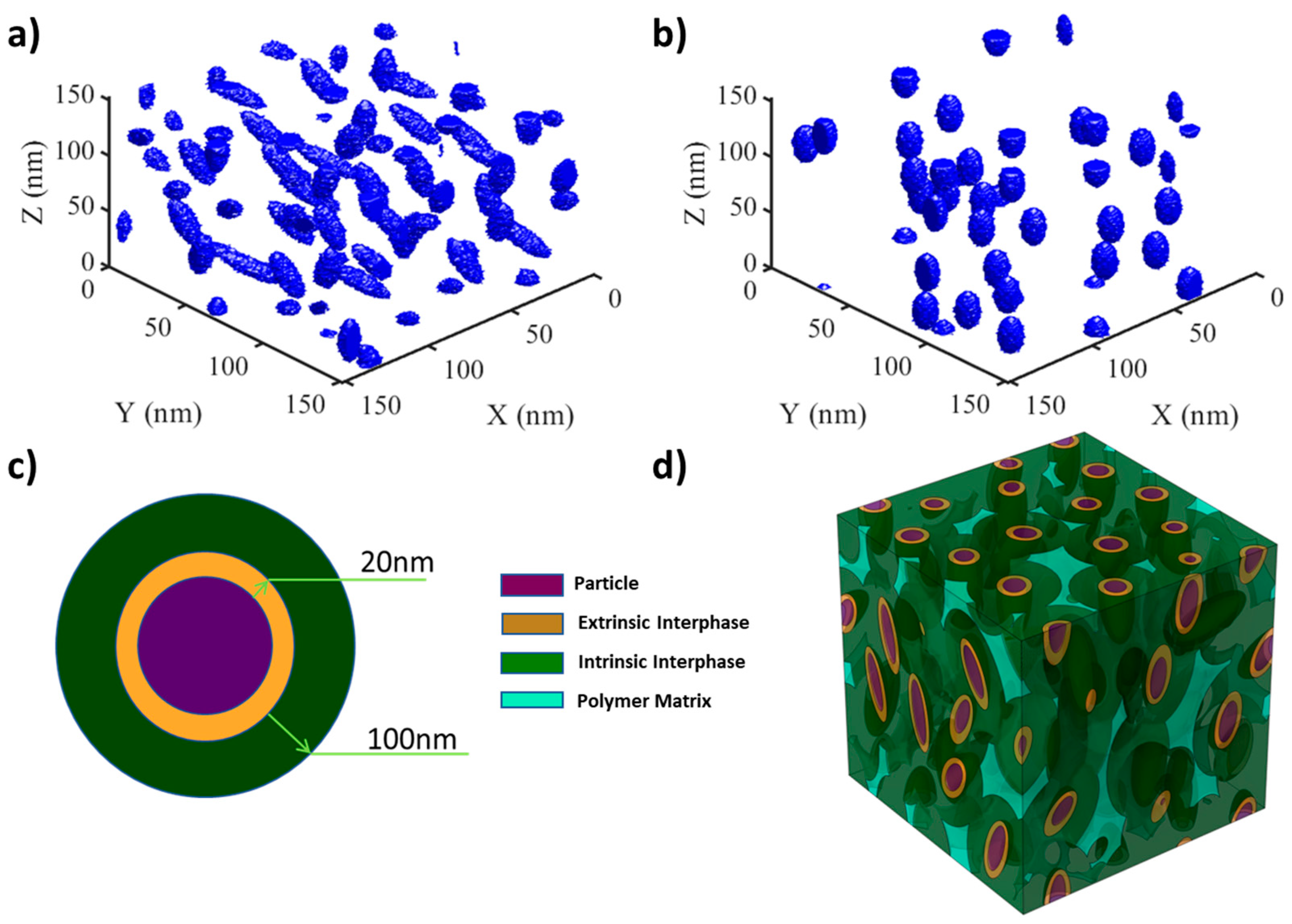
Microstructure Characterization and Reconstruction
Interfacial Layers
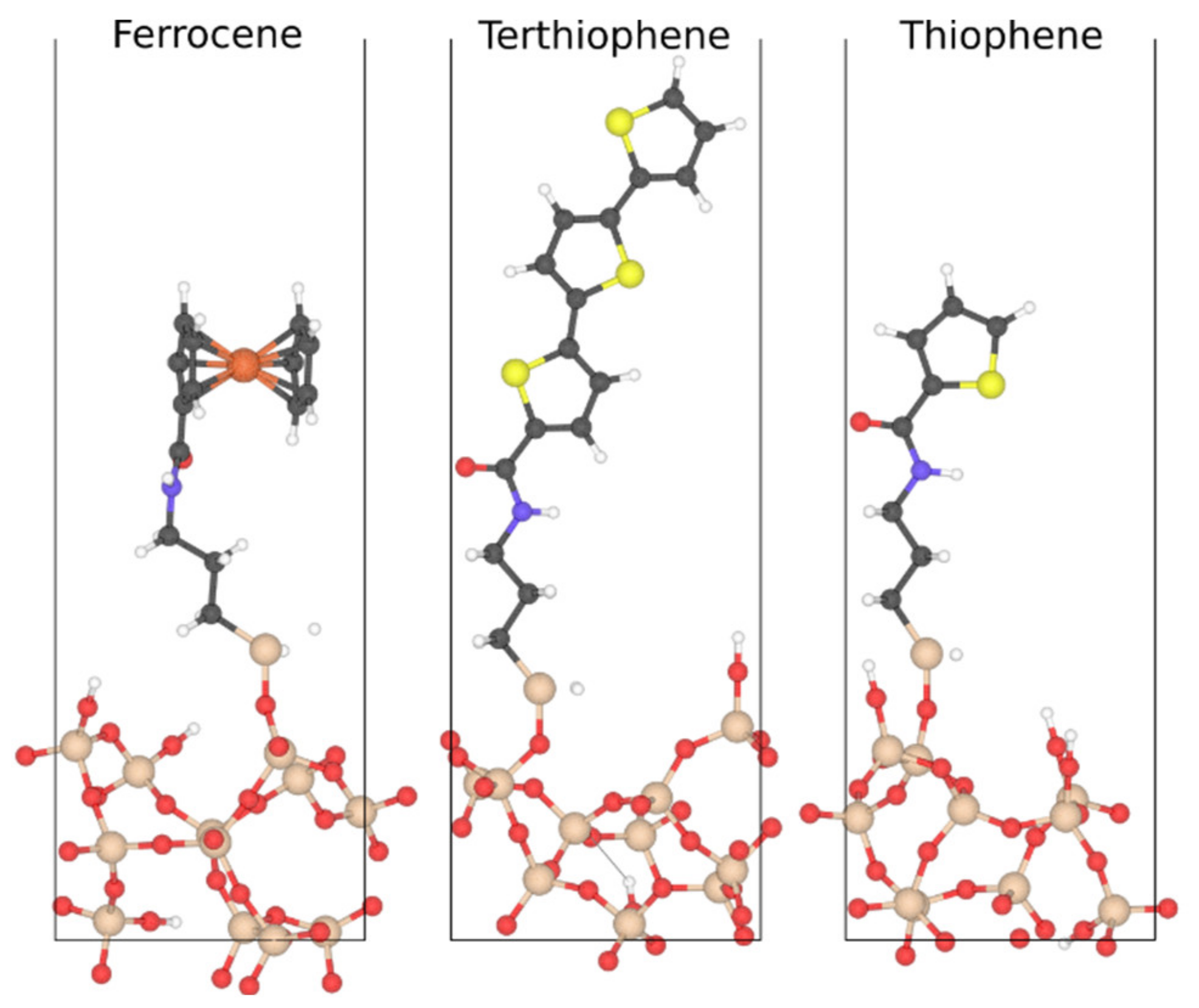
Extrinsic Interface
Intrinsic Interface
2.2.3. Property Evaluation: Physics-Based Simulation Methods
Breakdown Strength Calculations
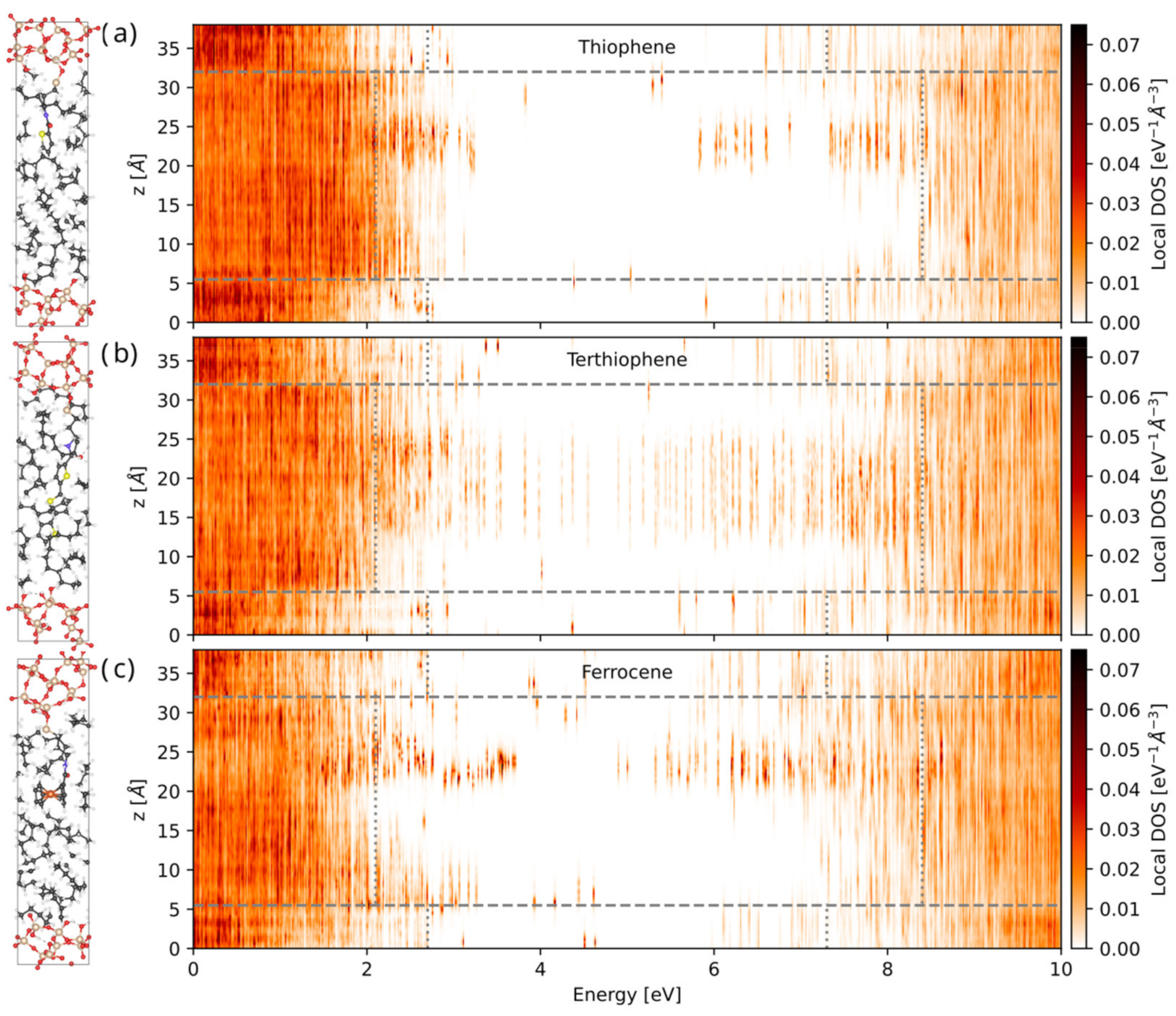
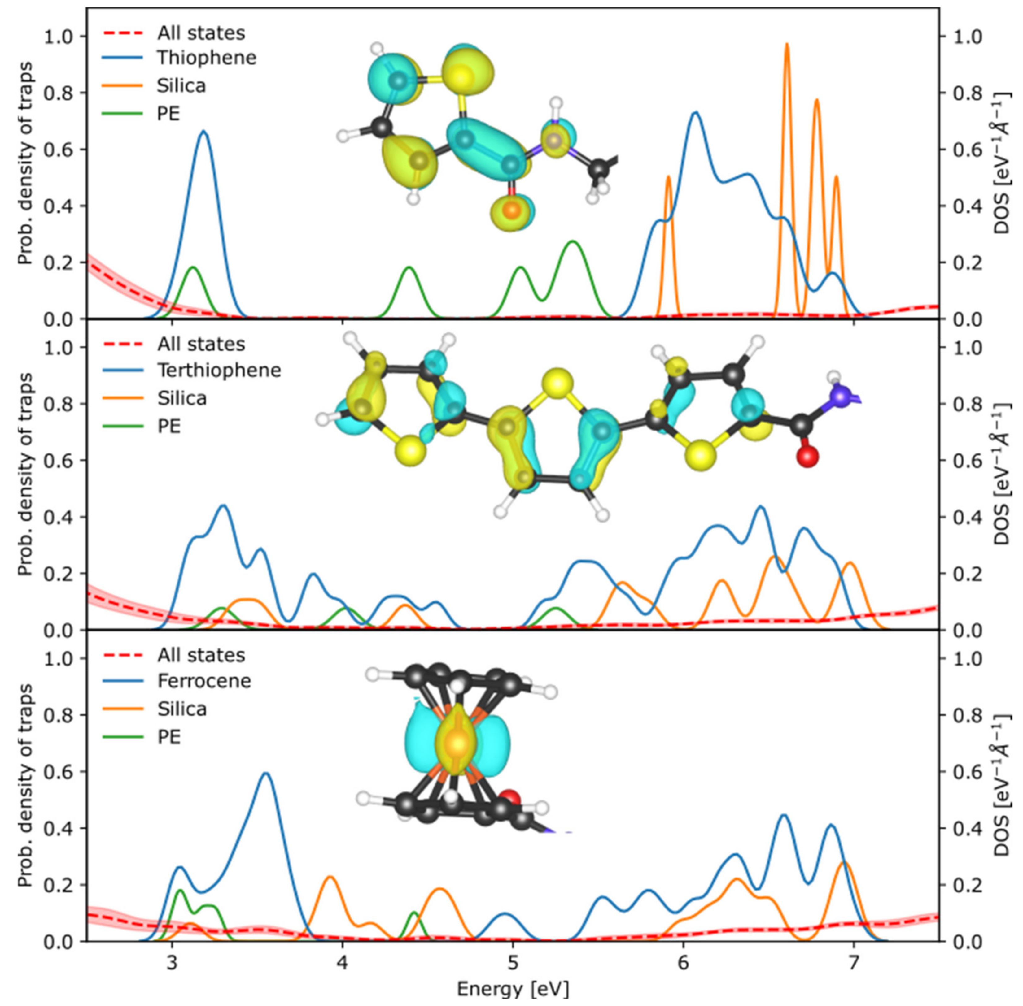
First-Principles Predictions of Trap States
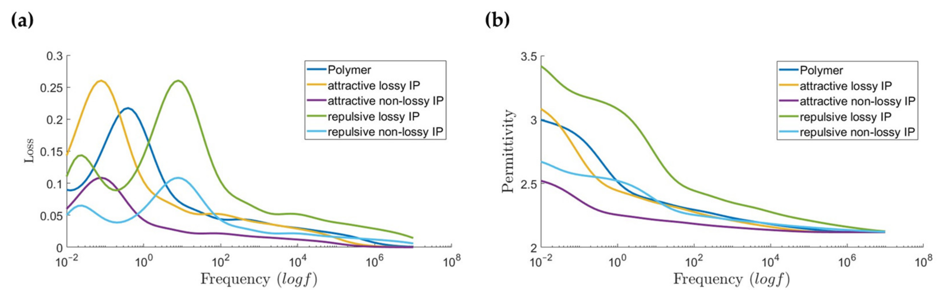
Permittivity and Loss Calculations
2.2.4. Metamodeling and Multi-Objective Optimization
Latent Variable Gaussian Process (LVGP) for Metamodeling
Bayesian Optimization
2.2.5. Design Analysis
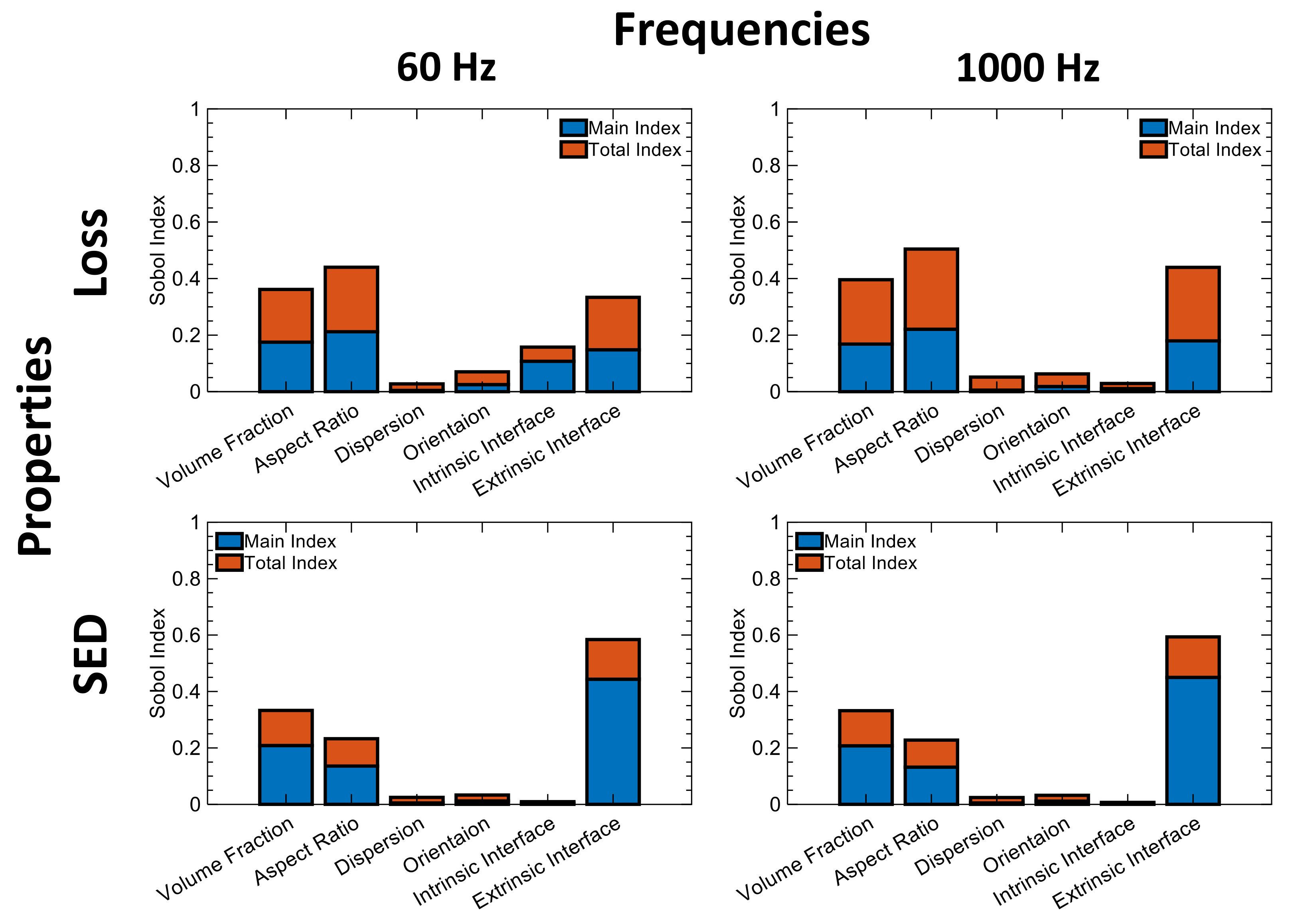
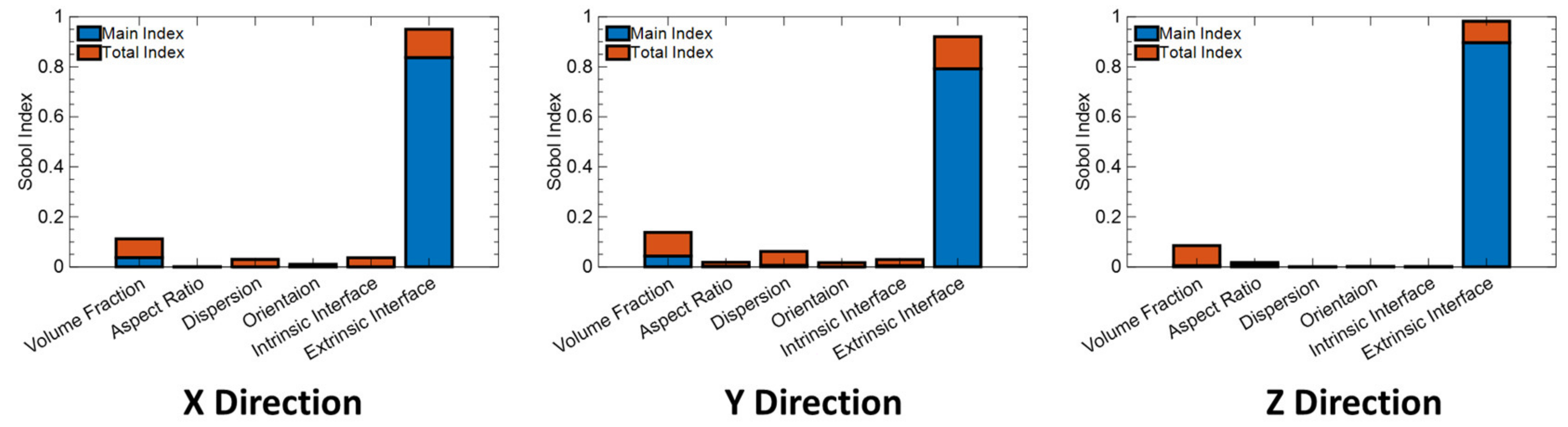
2.3. Global Sensitivity Analysis for the Mixed-Variable Design Space
3. Results
3.1. Initial Design of Experiments (DOE)
Global Sensitivity Analysis
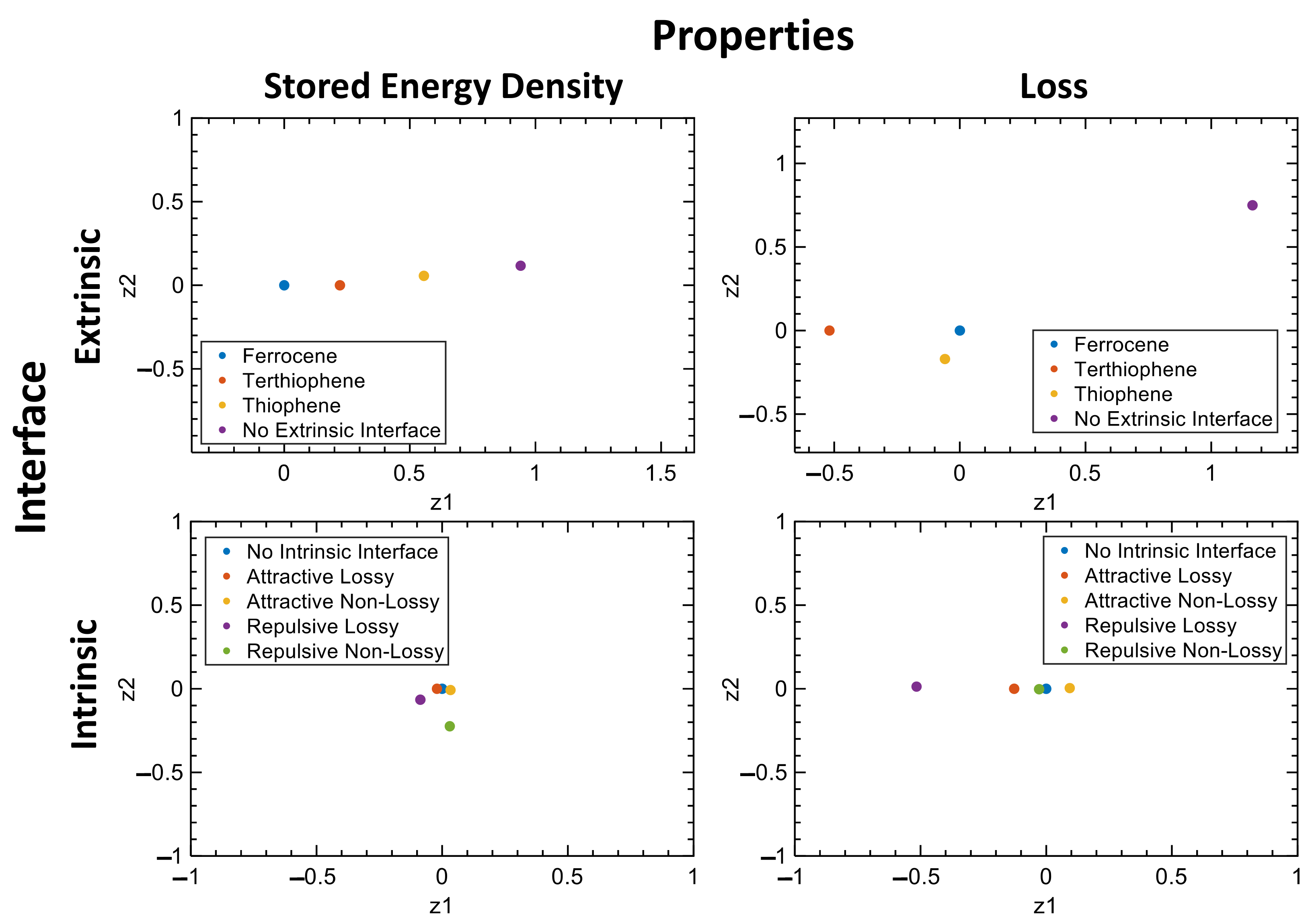
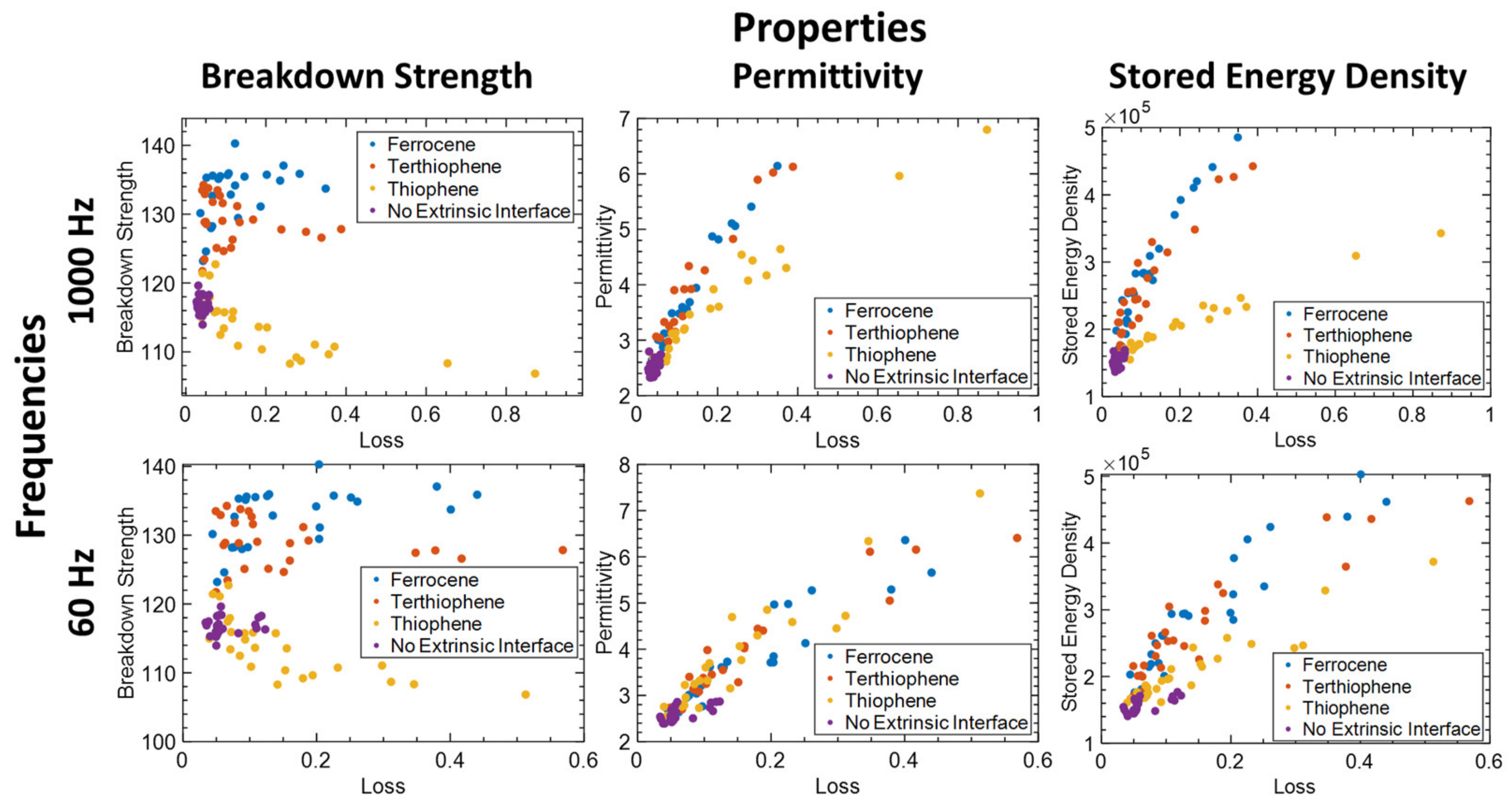
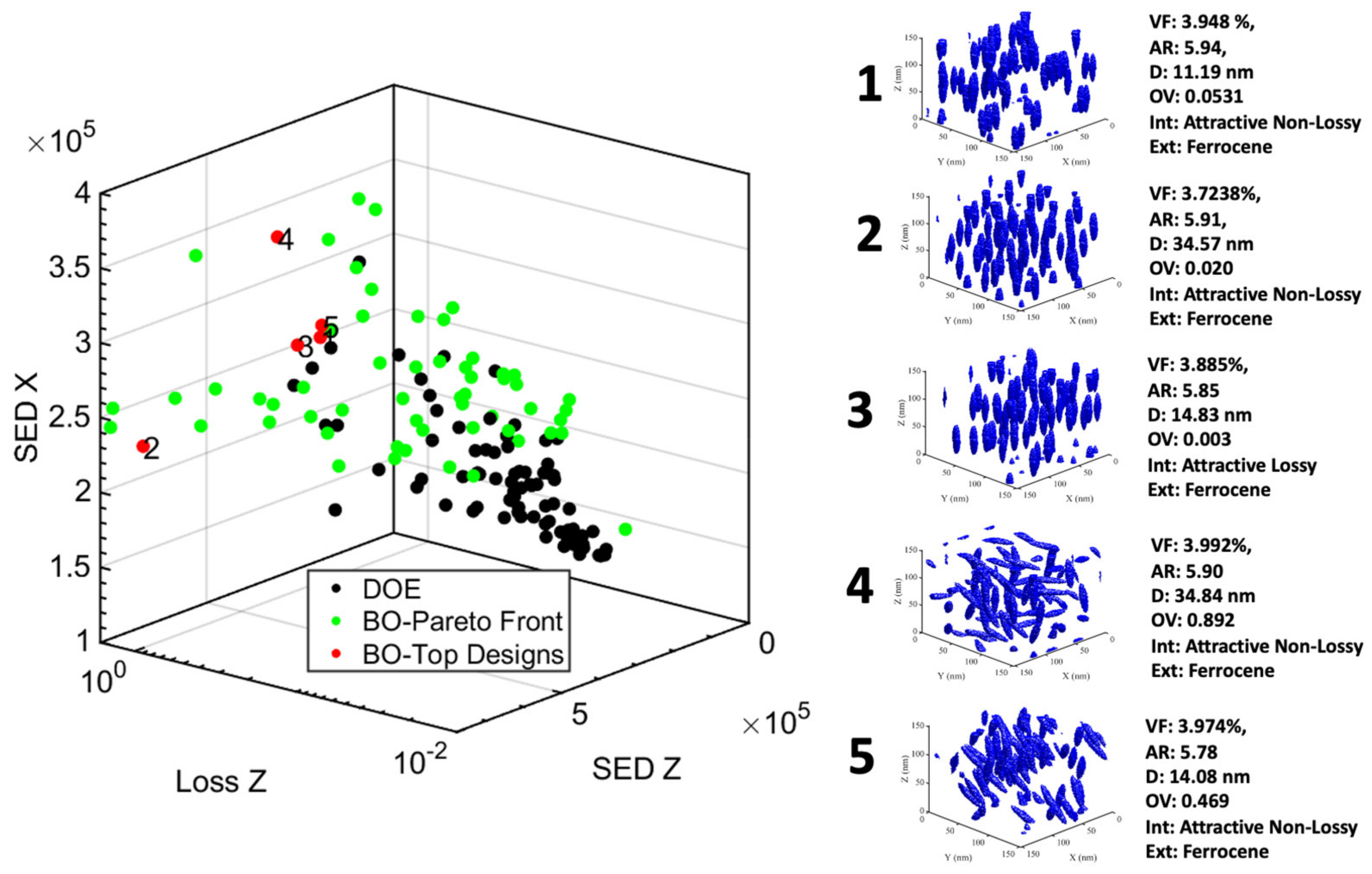
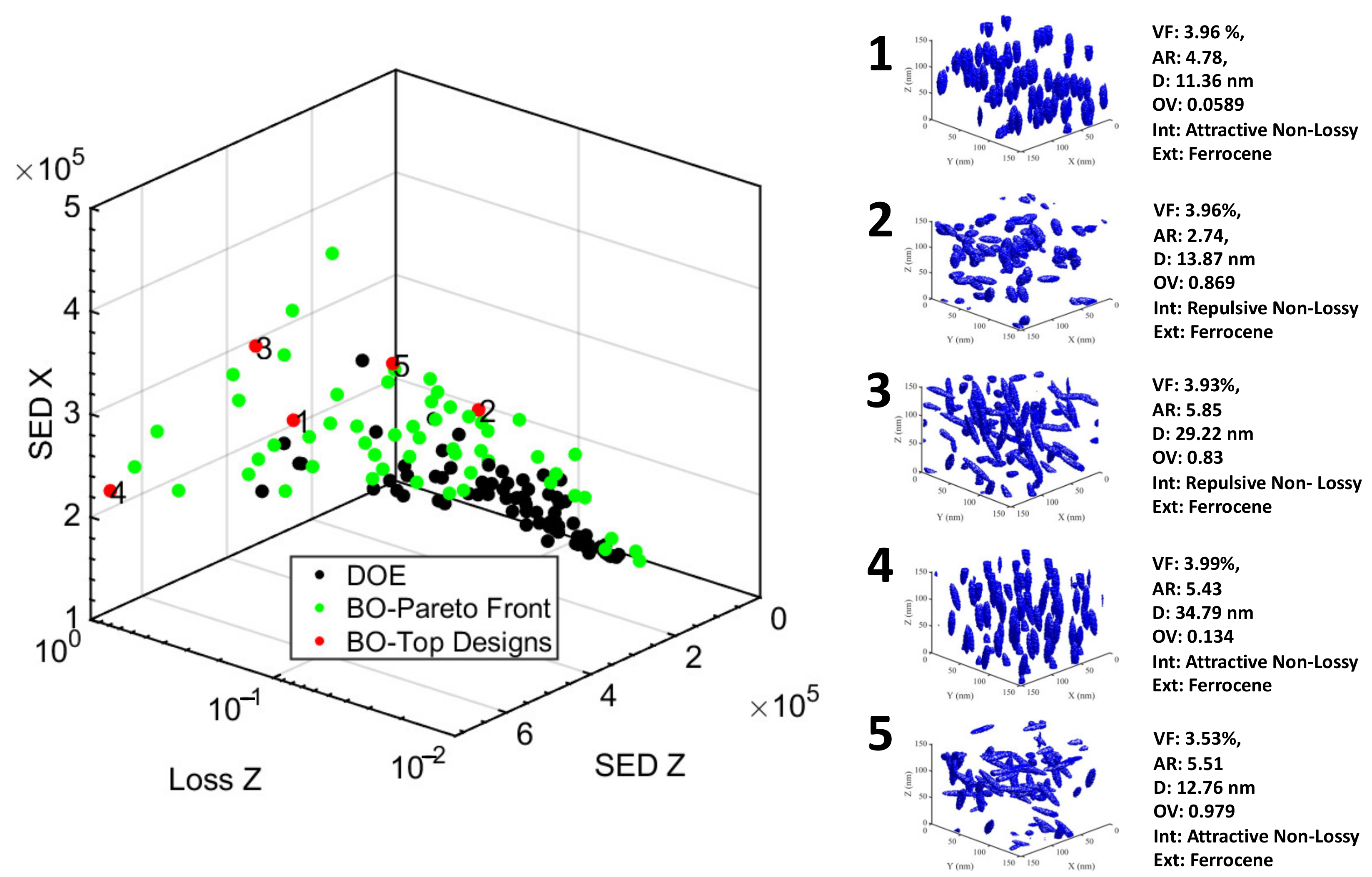
3.2. Nanodielectrics Design Optimization
4. Discussion
Supplementary Materials
Author Contributions
Funding
Data Availability Statement
Acknowledgments
Conflicts of Interest
Appendix A. Latent Variable Gaussian Process (LVGP) Modeling
References
- Zhang, G.; Li, Q.; Allahyarov, E.; Li, Y.; Zhu, L. Challenges and Opportunities of Polymer Nanodielectrics for Capacitive Energy Storage. ACS Appl. Mater. Interfaces 2021, 13, 37939–37960. [Google Scholar] [CrossRef] [PubMed]
- Wang, S.; Huang, X.; Wang, G.; Wang, Y.; He, J.; Jiang, P. Increasing the Energy Efficiency and Breakdown Strength of High-Energy-Density Polymer Nanocomposites by Engineering the Ba0.7Sr0.3TiO3 Nanowire Surface via Reversible Addition–Fragmentation Chain Transfer Polymerization. J. Phys. Chem. C 2015, 119, 25307–25318. [Google Scholar] [CrossRef]
- Li, Q.; Xue, Q.; Hao, L.; Gao, X.; Zheng, Q. Large dielectric constant of the chemically functionalized carbon nanotube/polymer composites. Compos. Sci. Technol. 2008, 68, 2290–2296. [Google Scholar] [CrossRef]
- Zhang, X.; Liang, G.; Chang, J.; Gu, A.; Yuan, L.; Zhang, W. The origin of the electric and dielectric behavior of expanded graphite–carbon nanotube/cyanate ester composites with very high dielectric constant and low dielectric loss. Carbon 2012, 50, 4995–5007. [Google Scholar] [CrossRef]
- Ning, N.; Bai, X.; Yang, D.; Zhang, L.; Lu, Y.; Nishi, T.; Tian, M. Dramatically improved dielectric properties of polymer composites by controlling the alignment of carbon nanotubes in matrix. RSC Adv. 2014, 4, 4543–4551. [Google Scholar] [CrossRef]
- Grabowski, C.A.; Fillery, S.P.; Koerner, H.; Tchoul, M.; Drummy, L.; Beier, C.W.; Brutchey, R.L.; Durstock, M.F.; Vaia, R.A. Dielectric performance of high permitivity nanocomposites: Impact of polystyrene grafting on BaTiO3 and TiO2. Nanocomposites 2016, 2, 117–124. [Google Scholar] [CrossRef]
- Kim, P.; Jones, S.C.; Hotchkiss, P.J.; Haddock, J.N.; Kippelen, B.; Marder, S.R.; Perry, J.W. Phosphonic Acid-Modified Barium Titanate Polymer Nanocomposites with High Permittivity and Dielectric Strength. Adv. Mater. 2007, 19, 1001–1005. [Google Scholar] [CrossRef]
- Siddabattuni, S.; Schuman, T.P.; Dogan, F. Dielectric Properties of Polymer–Particle Nanocomposites Influenced by Electronic Nature of Filler Surfaces. ACS Appl. Mater. Interfaces 2013, 5, 1917–1927. [Google Scholar] [CrossRef]
- Zhang, G.; Brannum, D.; Dong, D.; Tang, L.; Allahyarov, E.; Tang, S.; Kodweis, K.; Lee, J.-K.; Zhu, L. Interfacial Polarization-Induced Loss Mechanisms in Polypropylene/BaTiO3 Nanocomposite Dielectrics. Chem. Mater. 2016, 28, 4646–4660. [Google Scholar] [CrossRef]
- Zdorovets, M.V.; Kozlovskiy, A.L.; Shlimas, D.I.; Borgekov, D.B. Phase transformations in FeCo—Fe2CoO4/Co3O4-spinel nanostructures as a result of thermal annealing and their practical application. J. Mater. Sci. Mater. Electron. 2021, 32, 16694–16705. [Google Scholar] [CrossRef]
- Trukhanov, A.V.; Trukhanov, S.V.; Panina, L.V.; Kostishyn, V.G.; Chitanov, D.N.; Kazakevich, I.y.S.; Trukhanov, A.V.; Turchenko, V.A.; Salem, M.M. Strong corelation between magnetic and electrical subsystems in diamagnetically substituted hexaferrites ceramics. Ceram. Int. 2017, 43, 5635–5641. [Google Scholar] [CrossRef]
- Sanida, A.; Stavropoulos, S.G.; Speliotis, T.; Psarras, G.C. Evaluating the multifunctional performance of polymer matrix nanodielectrics incorporating magnetic nanoparticles: A comparative study. Polymer 2021, 236, 124311. [Google Scholar] [CrossRef]
- Zhou, W.; Cao, G.; Yuan, M.; Zhong, S.; Wang, Y.; Liu, X.; Cao, D.; Peng, W.; Liu, J.; Wang, G.; et al. Core-Shell Engineering of Conductive Fillers toward Enhanced Dielectric Properties: A Universal Polarization Mechanism in Polymer Conductor Composites. Adv. Mater. 2023, 35, e2207829. [Google Scholar] [CrossRef] [PubMed]
- Zhou, W.; Li, T.; Yuan, M.; Li, B.; Zhong, S.; Li, Z.; Liu, X.; Zhou, J.; Wang, Y.; Cai, H.; et al. Decoupling of inter-particle polarization and intra-particle polarization in core-shell structured nanocomposites towards improved dielectric performance. Energy Storage Mater. 2021, 42, 1–11. [Google Scholar] [CrossRef]
- Schadler, L.S. 6.3 The Elusive Interphase/Interface in Polymer Nanocomposites. In Comprehensive Composite Materials II; Beaumont, P.W.R., Zweben, C.H., Eds.; Elsevier: Oxford, UK, 2018; pp. 52–72. [Google Scholar]
- Gupta, P.; Schadler, L.S.; Sundararaman, R. Dielectric properties of polymer nanocomposite interphases from electrostatic force microscopy using machine learning. Mater. Charact. 2021, 173, 110909. [Google Scholar] [CrossRef]
- Zhang, M.; Askar, S.; Torkelson, J.M.; Brinson, L.C. Stiffness Gradients in Glassy Polymer Model Nanocomposites: Comparisons of Quantitative Characterization by Fluorescence Spectroscopy and Atomic Force Microscopy. Macromolecules 2017, 50, 5447–5458. [Google Scholar] [CrossRef]
- Qiao, R.; Catherine Brinson, L. Simulation of interphase percolation and gradients in polymer nanocomposites. Compos. Sci. Technol. 2009, 69, 491–499. [Google Scholar] [CrossRef]
- Qiao, R.; Deng, H.; Putz, K.W.; Brinson, L.C. Effect of particle agglomeration and interphase on the glass transition temperature of polymer nanocomposites. J. Polym. Sci. Part B Polym. Phys. 2011, 49, 740–748. [Google Scholar] [CrossRef]
- Huang, Y.; Krentz, T.M.; Nelson, J.K.; Schadler, L.S.; Li, Y.; Zhao, H.; Brinson, L.C.; Bell, M.; Benicewicz, B.; Wu, K.; et al. Prediction of interface dielectric relaxations in bimodal brush functionalized epoxy nanodielectrics by finite element analysis method. In Proceedings of the 2014 IEEE Conference on Electrical Insulation and Dielectric Phenomena (CEIDP), Des Moines, IA, USA, 19–22 October 2014; pp. 748–751. [Google Scholar]
- Li, X.; Zhang, M.; Wang, Y.; Zhang, M.; Prasad, A.; Chen, W.; Schadler, L.; Brinson, L.C. Rethinking interphase representations for modeling viscoelastic properties for polymer nanocomposites. Materialia 2019, 6, 100277. [Google Scholar] [CrossRef]
- Wang, Y.; Zhang, Y.; Zhao, H.; Li, X.; Huang, Y.; Schadler, L.S.; Chen, W.; Brinson, L.C. Identifying interphase properties in polymer nanocomposites using adaptive optimization. Compos. Sci. Technol. 2018, 162, 146–155. [Google Scholar] [CrossRef]
- Zhao, H.; Li, Y.; Brinson, L.C.; Huang, Y.; Krentz, T.M.; Schadler, L.S.; Bell, M.; Benicewicz, B. Dielectric spectroscopy analysis using viscoelasticity-inspired relaxation theory with finite element modeling. IEEE Trans. Dielectr. Electr. Insul. 2017, 24, 3776–3785. [Google Scholar] [CrossRef]
- Natarajan, B.; Li, Y.; Deng, H.; Brinson, L.C.; Schadler, L.S. Effect of Interfacial Energetics on Dispersion and Glass Transition Temperature in Polymer Nanocomposites. Macromolecules 2013, 46, 2833–2841. [Google Scholar] [CrossRef]
- Virtanen, S.; Krentz, T.M.; Nelson, J.K.; Schadler, L.S.; Bell, M.; Benicewicz, B.; Hillborg, H.; Zhao, S. Dielectric breakdown strength of epoxy bimodal-polymer-brush-grafted core functionalized silica nanocomposites. IEEE Trans. Dielectr. Electr. Insul. 2014, 21, 563–570. [Google Scholar] [CrossRef]
- Prasad, A.S.; Wang, Y.; Li, X.; Iyer, A.; Chen, W.; Brinson, L.C.; Schadler, L.S. Investigating the effect of surface modification on the dispersion process of polymer nanocomposites. Nanocomposites 2020, 6, 111–124. [Google Scholar] [CrossRef]
- Bell, M.; Krentz, T.; Keith Nelson, J.; Schadler, L.; Wu, K.; Breneman, C.; Zhao, S.; Hillborg, H.; Benicewicz, B. Investigation of dielectric breakdown in silica-epoxy nanocomposites using designed interfaces. J. Colloid Interface Sci. 2017, 495, 130–139. [Google Scholar] [CrossRef] [PubMed]
- Huang, Y.; Wu, K.; Bell, M.; Oakes, A.; Ratcliff, T.; Lanzillo, N.A.; Breneman, C.; Benicewicz, B.C.; Schadler, L.S. The effects of nanoparticles and organic additives with controlled dispersion on dielectric properties of polymers: Charge trapping and impact excitation. J. Appl. Phys. 2016, 120, 055102. [Google Scholar] [CrossRef]
- Krentz, T.M.; Huang, Y.; Nelson, J.K.; Schadler, L.S.; Bell, M.; Benicewicz, B.; Zhao, S.; Hillborg, H. Enhanced charge trapping in bimodal brush functionalized silica-epoxy nanocomposite dielectrics. In Proceedings of the 2014 IEEE Conference on Electrical Insulation and Dielectric Phenomena (CEIDP), Des Moines, IA, USA, 19–22 October 2014; pp. 643–646. [Google Scholar]
- Krentz, T.; Khani, M.M.; Bell, M.; Benicewicz, B.C.; Nelson, J.K.; Zhao, S.; Hillborg, H.; Schadler, L.S. Morphologically dependent alternating-current and direct-current breakdown strength in silica–polypropylene nanocomposites. J. Appl. Polym. Sci. 2017, 134. [Google Scholar] [CrossRef]
- Roy, M.; Nelson, J.K.; MacCrone, R.K.; Schadler, L.S. Candidate mechanisms controlling the electrical characteristics of silica/XLPE nanodielectrics. J. Mater. Sci. 2007, 42, 3789–3799. [Google Scholar] [CrossRef]
- Chen, W.; Schadler, L.; Brinson, C.; Wang, Y.; Zhang, Y.; Prasad, A.; Li, X.; Iyer, A. Materials Informatics and Data System for Polymer Nanocomposites Analysis and Design. In Handbook on Big Data and Machine Learning in the Physical Sciences; World Scientific Publishing: Hackensack, NJ, USA, 2020; pp. 65–125. [Google Scholar]
- Wang, Y.; Zhang, M.; Lin, A.; Iyer, A.; Prasad, A.S.; Li, X.; Zhang, Y.; Schadler, L.S.; Chen, W.; Brinson, L.C. Mining structure–property relationships in polymer nanocomposites using data driven finite element analysis and multi-task convolutional neural networks. Mol. Syst. Des. Eng. 2020, 5, 962–975. [Google Scholar] [CrossRef]
- Schadler, L.S.; Chen, W.; Brinson, L.C.; Sundararaman, R.; Gupta, P.; Prabhune, P.; Iyer, A.; Wang, Y.; Shandilya, A. A perspective on the data-driven design of polymer nanodielectrics. J. Phys. D Appl. Phys. 2020, 53, 333001. [Google Scholar] [CrossRef]
- Iyer, A.; Zhang, Y.; Prasad, A.; Gupta, P.; Tao, S.; Wang, Y.; Prabhune, P.; Schadler, L.S.; Brinson, L.C.; Chen, W. Data centric nanocomposites design via mixed-variable Bayesian optimization. Mol. Syst. Des. Eng. 2020, 5, 1376–1390. [Google Scholar] [CrossRef]
- Schadler, L.S.; Chen, W.; Brinson, L.C.; Sundararaman, R.; Prabhune, P.; Iyer, A. (Invited) Combining Machine Learning, DFT, EFM, and Modeling to Design Nanodielectric Behavior. ECS Trans. 2022, 108, 51. [Google Scholar] [CrossRef]
- Ba, S.; Myers, W.R.; Brenneman, W.A. Optimal Sliced Latin Hypercube Designs. Technometrics 2015, 57, 479–487. [Google Scholar] [CrossRef]
- Wang, W.; Wang, J.; Kim, M.-S. An algebraic condition for the separation of two ellipsoids. Comput. Aided Geom. Des. 2001, 18, 531–539. [Google Scholar] [CrossRef]
- Shandilya, A.; Schadler, L.S.; Sundararaman, R. First-principles identification of localized trap states in polymer nanocomposite interfaces. J. Mater. Res. 2020, 35, 931–939. [Google Scholar] [CrossRef]
- Sundararaman, R.; Letchworth-Weaver, K.; Schwarz, K.A.; Gunceler, D.; Ozhabes, Y.; Arias, T.A. JDFTx: Software for joint density-functional theory. SoftwareX 2017, 6, 278–284. [Google Scholar] [CrossRef] [PubMed]
- Perdew, J.P.; Burke, K.; Ernzerhof, M. Generalized Gradient Approximation Made Simple. Phys. Rev. Lett. 1996, 77, 3865–3868. [Google Scholar] [CrossRef]
- Garrity, K.F.; Bennett, J.W.; Rabe, K.M.; Vanderbilt, D. Pseudopotentials for high-throughput DFT calculations. Comput. Mater. Sci. 2014, 81, 446–452. [Google Scholar] [CrossRef]
- Zhang, Y.; Tao, S.; Chen, W.; Apley, D.W. A Latent Variable Approach to Gaussian Process Modeling with Qualitative and Quantitative Factors. Technometrics 2020, 62, 291–302. [Google Scholar] [CrossRef]
- Zhang, Y.; Apley, D.W.; Chen, W. Bayesian Optimization for Materials Design with Mixed Quantitative and Qualitative Variables. Sci. Rep. 2020, 10, 4924. [Google Scholar] [CrossRef]
- Wang, Y.; Iyer, A.; Chen, W.; Rondinelli, J.M. Featureless adaptive optimization accelerates functional electronic materials design. Appl. Phys. Rev. 2020, 7, 041403. [Google Scholar] [CrossRef]
- Comlek, Y.; Pham, T.D.; Snurr, R.; Chen, W. Rapid Design of Top-Performing Metal-Organic Frameworks with Qualitative Representations of Building Blocks. arXiv 2023, arXiv:2302.09184. [Google Scholar]
- Sobol′, I.M. Global sensitivity indices for nonlinear mathematical models and their Monte Carlo estimates. Math. Comput. Simul. 2001, 55, 271–280. [Google Scholar] [CrossRef]
- Comlek, Y.; Wang, L.; Chen, W. Mixed-variable global sensitivity analysis with applications to data-driven combinatorial materials design. In International Design Engineering Technical Conferences and Computers and Information in Engineering Conference; Paper Number: IDETC2023-110756; American Society of Mechanical Engineers: New York, NY, USA, 2023. [Google Scholar]
- Yu, K.; Wang, H.; Zhou, Y.; Bai, Y.; Niu, Y. Enhanced dielectric properties of BaTiO3/poly(vinylidene fluoride) nanocomposites for energy storage applications. J. Appl. Phys. 2013, 113, 034105. [Google Scholar] [CrossRef]
- Li, B.; Randall, C.A.; Manias, E. Polarization Mechanism Underlying Strongly Enhanced Dielectric Permittivity in Polymer Composites with Conductive Fillers. J. Phys. Chem. C 2022, 126, 7596–7604. [Google Scholar] [CrossRef]
- Carroll, B.; Cheng, S.; Sokolov, A.P. Analyzing the Interfacial Layer Properties in Polymer Nanocomposites by Broadband Dielectric Spectroscopy. Macromolecules 2017, 50, 6149–6163. [Google Scholar] [CrossRef]
- Holt, A.P.; Griffin, P.J.; Bocharova, V.; Agapov, A.L.; Imel, A.E.; Dadmun, M.D.; Sangoro, J.R.; Sokolov, A.P. Dynamics at the Polymer/Nanoparticle Interface in Poly(2-vinylpyridine)/Silica Nanocomposites. Macromolecules 2014, 47, 1837–1843. [Google Scholar] [CrossRef]
- Cheng, S.; Mirigian, S.; Carrillo, J.-M.Y.; Bocharova, V.; Sumpter, B.G.; Schweizer, K.S.; Sokolov, A.P. Revealing spatially heterogeneous relaxation in a model nanocomposite. J. Chem. Phys. 2015, 143, 194704. [Google Scholar] [CrossRef]


| Design Variables | Design Choices | |
|---|---|---|
| Microstructural (Quantitative) | Volume Fraction (VF) | (1,4)% |
| Aspect Ratio (AR) | (1–6) | |
| Dispersion (D) | (11–36) nm | |
| Orientation Variation (OV) | (0,1) | |
| Interfacial (Qualitative) | Intrinsic Interface | Attractive Lossy, Attractive Non-Lossy, Repulsive Lossy, Repulsive Non-Lossy, No Interface |
| Extrinsic Interface | Ferrocene, Terthiophene, Thiophene, No Interface (No Extrinsic Interface) |
| # | Ligand Molecule | Conductivity |
|---|---|---|
| 1 | Thiophene | 1 × 10⁻¹⁰ |
| 2 | Terthiophene | 1 × 10⁻⁷ |
| 3 | Ferrocene | 1 × 10⁻¹ |
| # | Intrinsic Interface | |||||
|---|---|---|---|---|---|---|
| 1 | Attractive Lossy (AL) | 5.0 | 1.2 | 7.0 | 1.1 | 0 |
| 2 | Attractive Non-Lossy (ANL) | 5.0 | 0.5 | 7.0 | 0.5 | 0 |
| 3 | Repulsive Lossy (RL) | 0.05 | 1.2 | 0.07 | 1.1 | 0 |
| 4 | Repulsive Non-Lossy (RNL) | 0.05 | 0.5 | 0.07 | 0.5 | 0 |
| 5 | No Intrinsic Interface | 1 | 1 | 1 | 1 | 0 |
| Properties/Directions | X | Y | Z |
|---|---|---|---|
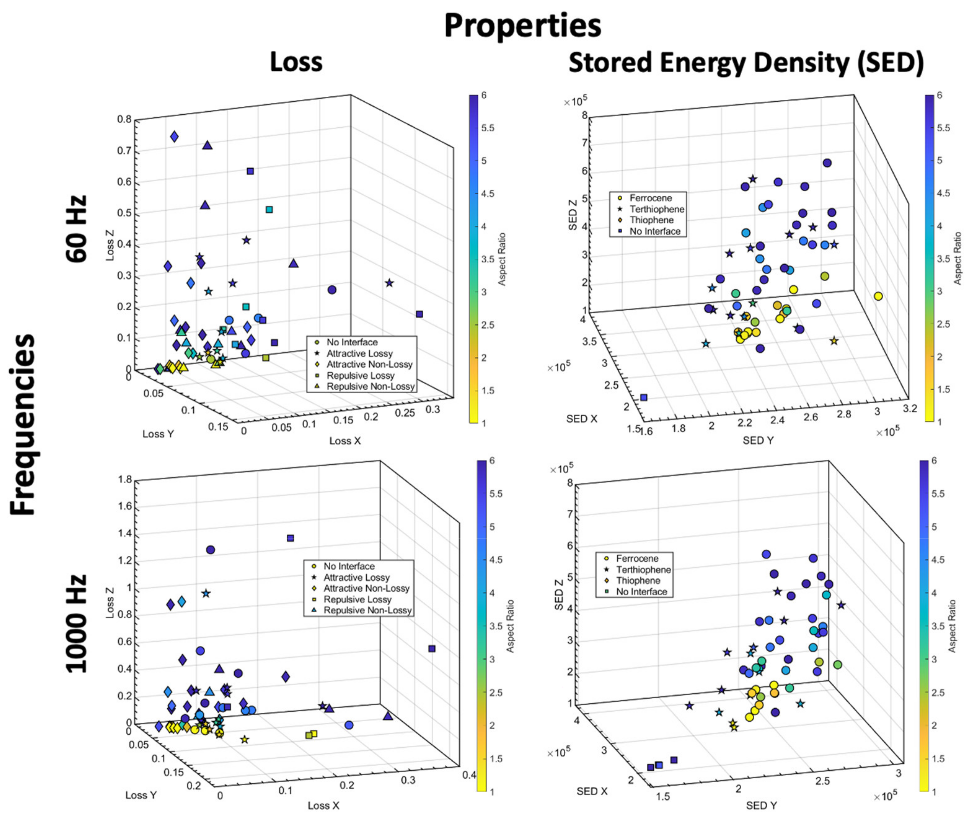
| Loss vs. Breakdown Strength | 0.21 | 0.2 | 0.12 |
| Loss vs. Permittivity | 0.78 | 0.7 | 0.93 |
| Loss vs. Stored Energy Density | 0.63 | 0.54 | 0.85 |
| Top Designs/Properties | Loss_x | Loss_y | Loss_z | |||
|---|---|---|---|---|---|---|
| 1 | 0.068 | 0.041 | 0.309 | 2976 | 2411 | 5060 |
| 2 | 0.038 | 0.035 | 0.943 | 2364 | 2325 | 7709 |
| 3 | 0.108 | 0.074 | 0.381 | 2921 | 2709 | 5276 |
| 4 | 0.194 | 0.090 | 0.460 | 3638 | 2854 | 5459 |
| 5 | 0.117 | 0.104 | 0.319 | 3043 | 2941 | 4952 |
| Top Designs/Properties | Loss_x | Loss_y | Loss_z | |||
|---|---|---|---|---|---|---|
| 1 | 0.055 | 0.033 | 0.300 | 2759 | 2432 | 4679 |
| 2 | 0.071 | 0.062 | 0.073 | 2880 | 2882 | 2931 |
| 3 | 0.179 | 0.074 | 0.376 | 3512 | 2885 | 5150 |
| 4 | 0.030 | 0.032 | 0.774 | 2316 | 2341 | 7238 |
| 5 | 0.107 | 0.077 | 0.153 | 3272 | 2828 | 3590 |
Disclaimer/Publisher’s Note: The statements, opinions and data contained in all publications are solely those of the individual author(s) and contributor(s) and not of MDPI and/or the editor(s). MDPI and/or the editor(s) disclaim responsibility for any injury to people or property resulting from any ideas, methods, instructions or products referred to in the content. |
© 2023 by the authors. Licensee MDPI, Basel, Switzerland. This article is an open access article distributed under the terms and conditions of the Creative Commons Attribution (CC BY) license (https://creativecommons.org/licenses/by/4.0/).
Share and Cite
Prabhune, P.; Comlek, Y.; Shandilya, A.; Sundararaman, R.; Schadler, L.S.; Brinson, L.C.; Chen, W. Design of Polymer Nanodielectrics for Capacitive Energy Storage. Nanomaterials 2023, 13, 2394. https://doi.org/10.3390/nano13172394
Prabhune P, Comlek Y, Shandilya A, Sundararaman R, Schadler LS, Brinson LC, Chen W. Design of Polymer Nanodielectrics for Capacitive Energy Storage. Nanomaterials. 2023; 13(17):2394. https://doi.org/10.3390/nano13172394
Chicago/Turabian StylePrabhune, Prajakta, Yigitcan Comlek, Abhishek Shandilya, Ravishankar Sundararaman, Linda S. Schadler, Lynda Catherine Brinson, and Wei Chen. 2023. "Design of Polymer Nanodielectrics for Capacitive Energy Storage" Nanomaterials 13, no. 17: 2394. https://doi.org/10.3390/nano13172394
APA StylePrabhune, P., Comlek, Y., Shandilya, A., Sundararaman, R., Schadler, L. S., Brinson, L. C., & Chen, W. (2023). Design of Polymer Nanodielectrics for Capacitive Energy Storage. Nanomaterials, 13(17), 2394. https://doi.org/10.3390/nano13172394