
Insight into the Role of Nanoparticles Shape Factors and Diameter on the Dynamics of Rotating Water-Based Fluid

 , , and
Abstract
:1. Introduction
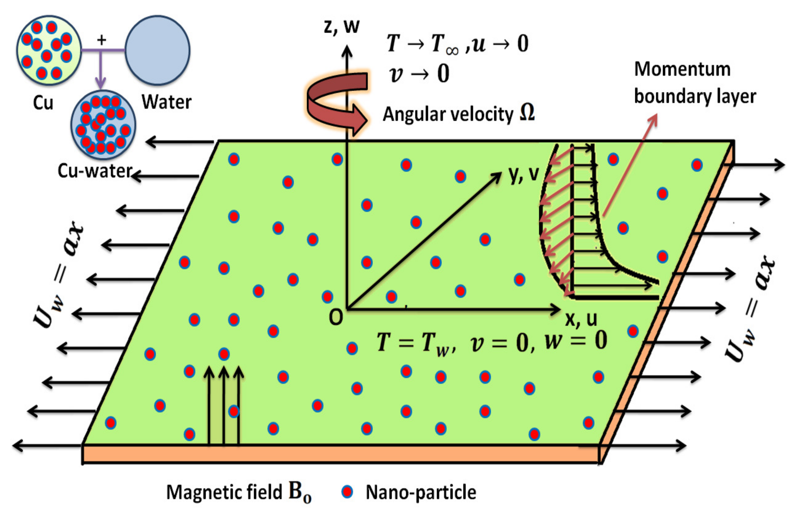
2. Mathematical Analysis and Flow Geometry
3. Numerical Procedure
4. Results and Discussion
5. Concluding Remarks
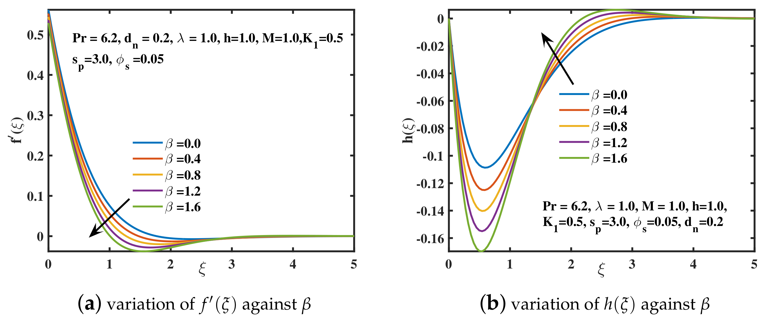
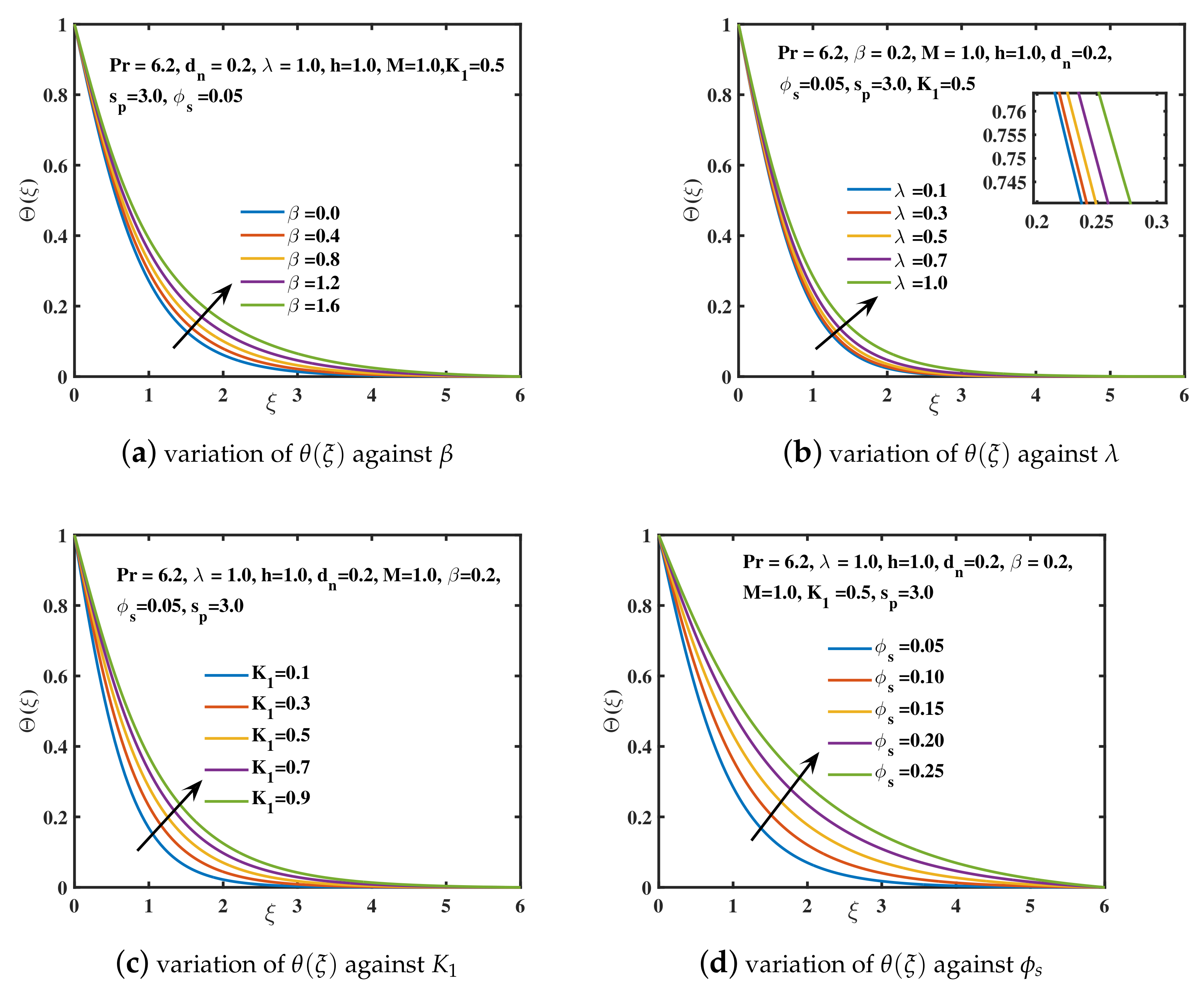
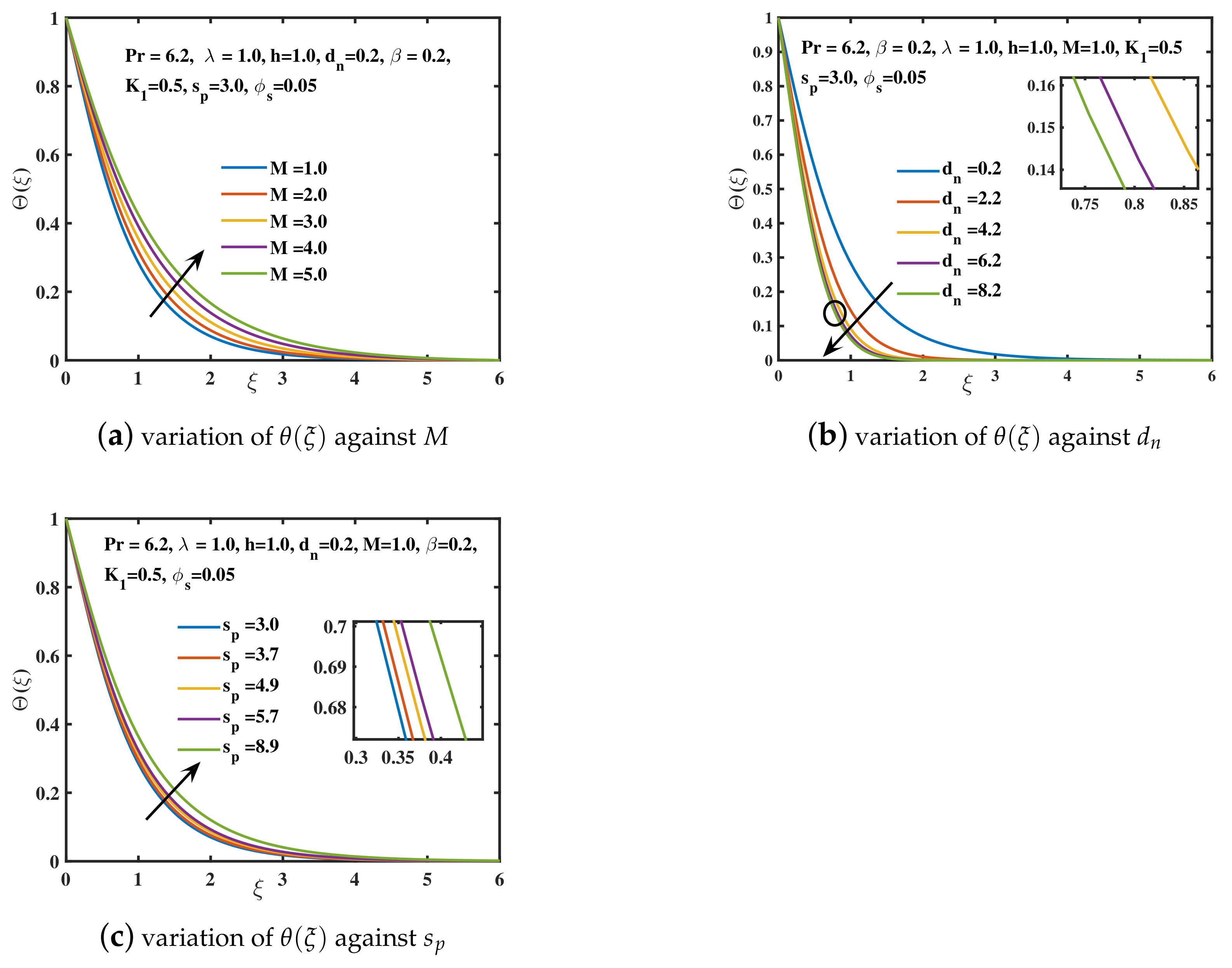
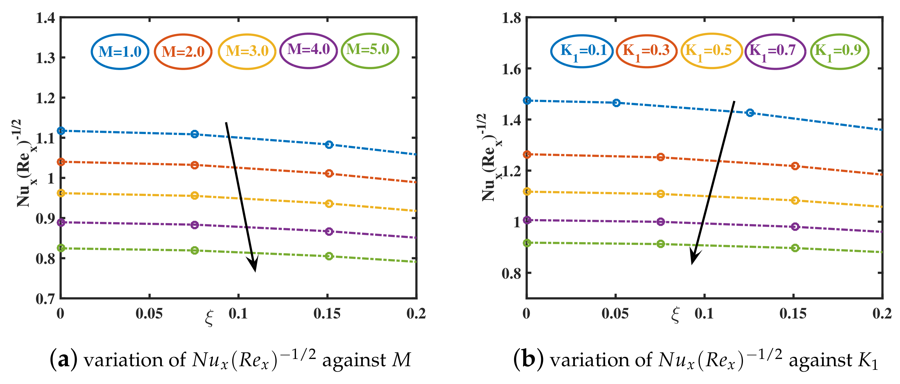
- The growing values of Deborah number and magnetic constant M have declined the velocity and the amplitude of velocity curve , while the progressing trend for the temperature curve is achieved.
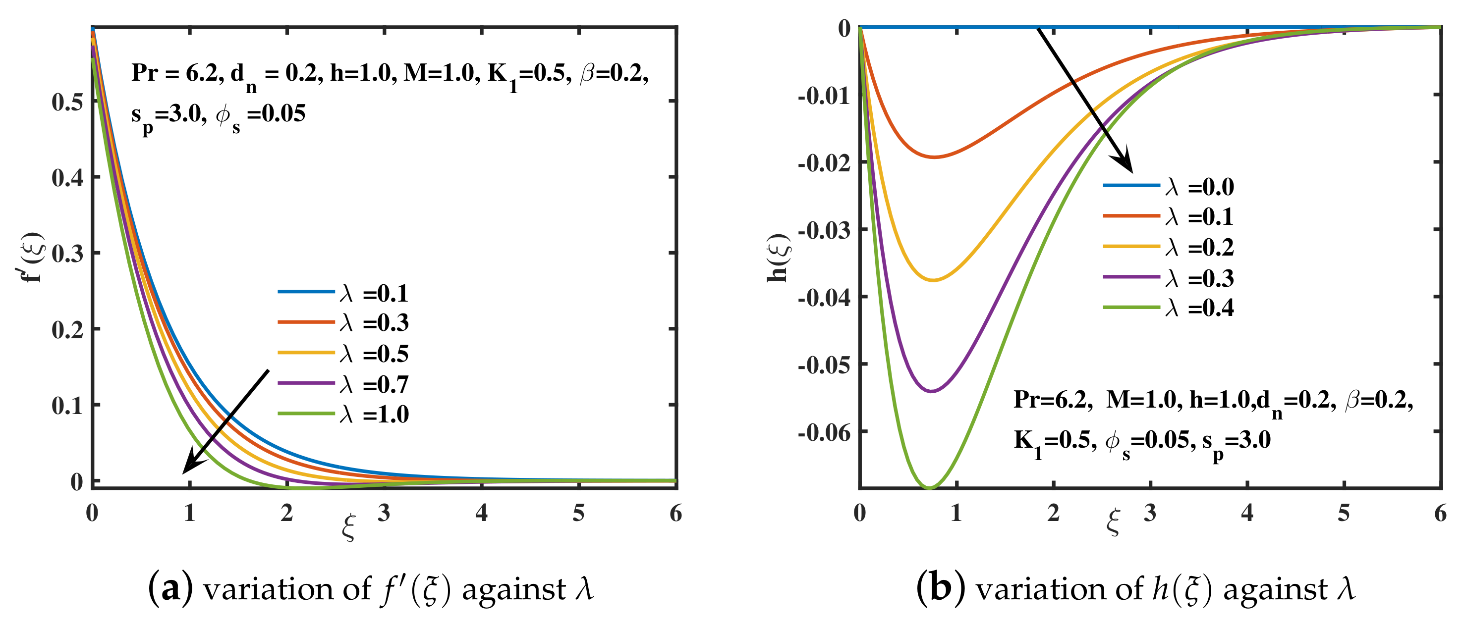
- The velocity along x and directions is decremented in the vicinity of the sheet for the exceeding rotational effects. An oscillating fashion is examined for larger rotational impacts. Ultimately, the hydraulic boundary layer depth is reduced. The temperature is incremented due to the enhanced kinetic energy of the nanofluid particles for the higher values.
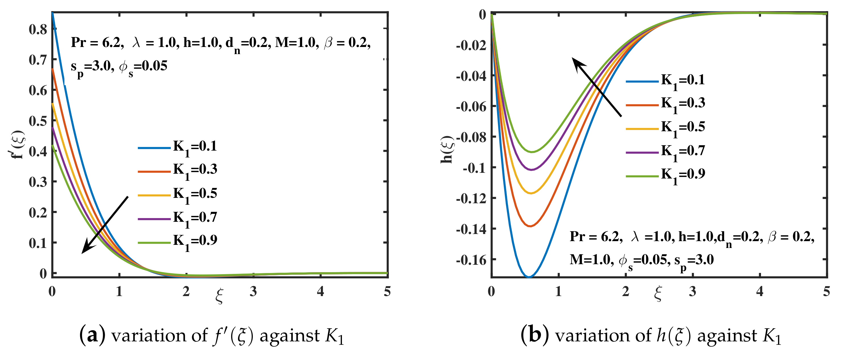
- Due to the slip boundary parameter , both the principle velocity and the amplitude of secondary velocity decreases while a growing behavior for the nanofluid temperature is observed.
- The improved velocity is induced by a reduction in the viscosity of water-based nanoliquid due to a larger diameter of copper nanoparticles. It is also feasible to get a significant decline in temperature distribution over the region by raising the diameter of copper nanoparticles.
- The increased retardation of nanofluid depreciates the component of velocity as well as the amplitude of the y-component of velocity for the addition of higher concentration of copper nanoparticles. An appreciating trend for is analyzed.
- The blade shape of copper nanoparticles is proved to be more effective for higher heat transport rates.
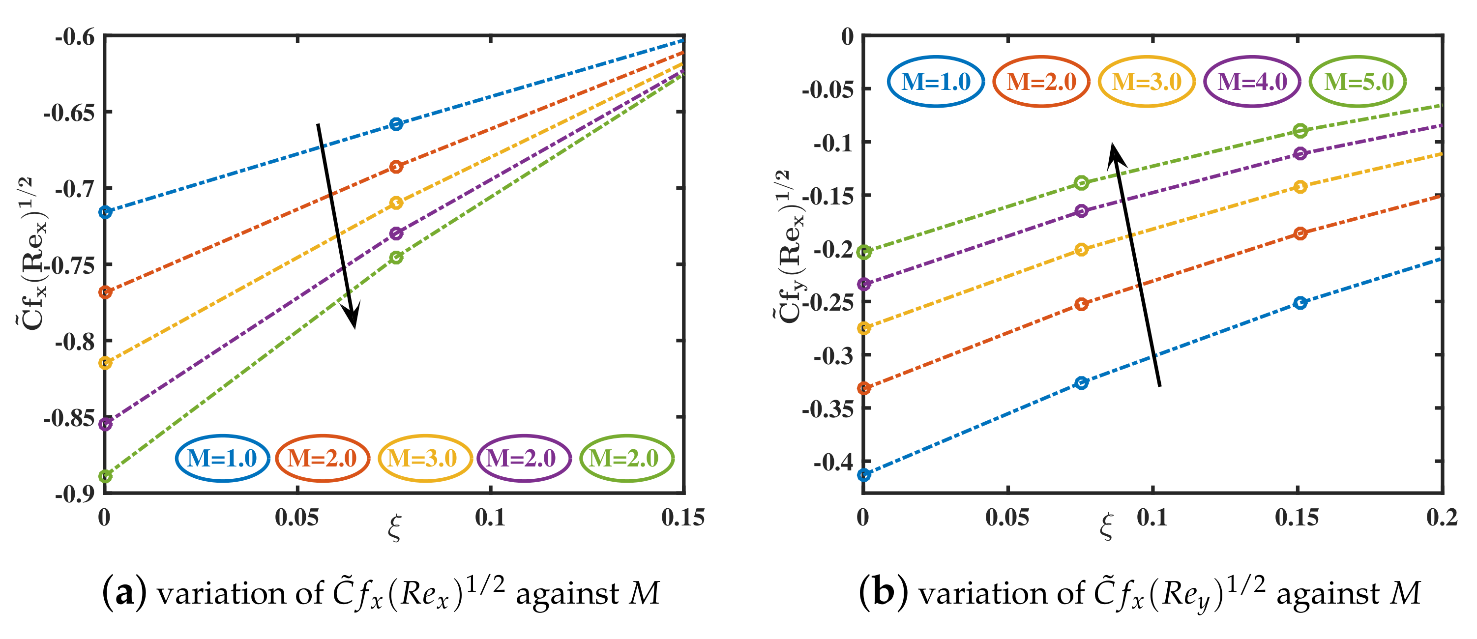
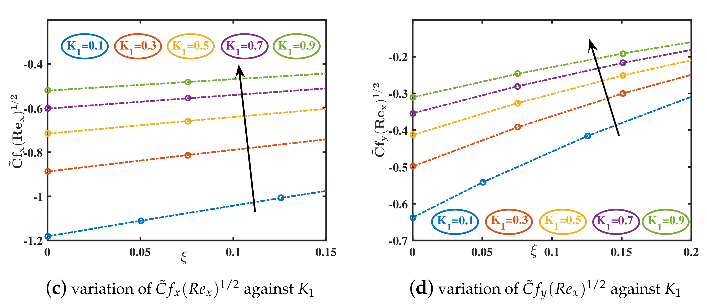
- The skin frictions gain lower values for the advancing values of and . A boosting fashion is obtained for the larger values of , and .
- The wall heat transport coefficient shows an ascending trend for higher values of nanoparticle diameter and shape . However, a reversing behavior is examined for the higher parametric values of , , M, , and .
Author Contributions
Funding
Institutional Review Board Statement
Informed Consent Statement
Data Availability Statement
Conflicts of Interest
Nomenclature
| cartesian coordinates (m) | (u, v, w) | constituents of velocity (m/s) | |
| applied magnetic field (kg/s·A) | T | fluid’s temperature (K) | |
| stretching velocity (m/s) | k | heat conductivity (W/m·K) | |
| a | stretching rate constant (1/s) | h | inter-particle spacing (m) |
| diameter of nanoparticle (m) | nanoparticle shape factor | ||
| dimensionless velocity in x-direction | dimensionless temperature | ||
| dimensionless velocity in y-direction | Prandtl number | ||
| M | magnetic parameter | slip parameter | |
| specific heat capacity (J/kg·K) | direction skin friction | ||
| y-direction skin friction | the local Nusselt number | ||
| heat flux through sheet (W/m) | temperature at wall (K) | ||
| ambient temperature (K) | Reynolds number | ||
| Greek symbols | |||
| density (kg/m) | viscosity (kg/m·s) | ||
| electrical conductance (A·s/kg·m) | angular velocity (1/s) | ||
| fluid’s relaxation time (s) | solid nanoparticle concentration | ||
| dimensionless variable | rotational parameter | ||
| Deborah number | kinematic viscosity (m/s) | ||
| Subscripts | |||
| f | base fluid | nanofluid | |
| s | solid nanoparticle |
References
- Karwe, M.; Jaluria, Y. Numerical simulation of thermal transport associated with a continuously moving flat sheet in materials processing. J. Heat Transfer 1991, 113, 612–619. [Google Scholar] [CrossRef]
- Ali, L.; Liu, X.; Ali, B.; Mujeed, S.; Abdal, S.; Khan, S.A. Analysis of magnetic properties of nano-particles due to a magnetic dipole in micropolar fluid flow over a stretching sheet. Coatings 2020, 10, 170. [Google Scholar] [CrossRef]
- Shah, S.A.A.; Ahammad, N.A.; Din, E.M.T.E.; Gamaoun, F.; Awan, A.U.; Ali, B. Bio-Convection Effects on Prandtl Hybrid Nanofluid Flow with Chemical Reaction and Motile Microorganism over a Stretching Sheet. Nanomaterials 2022, 12, 2174. [Google Scholar] [CrossRef] [PubMed]
- Crane, L.J. Flow past a stretching plate. Z. Angew. Math. Phys. 1970, 21, 645–647. [Google Scholar] [CrossRef]
- Wang, C. Stagnation flow towards a shrinking sheet. Int. J. Non-Linear Mech. 2008, 43, 377–382. [Google Scholar] [CrossRef]
- Hayat, T.; Ullah, I.; Alsaedi, A.; Farooq, M. MHD flow of Powell-Eyring nanofluid over a non-linear stretching sheet with variable thickness. Results Phys. 2017, 7, 189–196. [Google Scholar] [CrossRef]
- Majeed, A.; Zeeshan, A.; Alamri, S.Z.; Ellahi, R. Heat transfer analysis in ferromagnetic viscoelastic fluid flow over a stretching sheet with suction. Neural. Comput. Appl. 2018, 30, 1947–1955. [Google Scholar] [CrossRef]
- Awan, A.U.; Abid, S.; Ullah, N.; Nadeem, S. Magnetohydrodynamic oblique stagnation point flow of second grade fluid over an oscillatory stretching surface. Results Phys. 2020, 18, 103233. [Google Scholar] [CrossRef]
- Awan, A.U.; Abid, S.; Abbas, N. Theoretical study of unsteady oblique stagnation point based Jeffrey nanofluid flow over an oscillatory stretching sheet. Adv. Mech. Eng. 2020, 12, 1687814020971881. [Google Scholar] [CrossRef]
- Awan, A.U.; Riaz, S.; Abro, K.A.; Siddiqa, A.; Ali, Q. The role of relaxation and retardation phenomenon of Oldroyd-B fluid flow through Stehfest and Tzou algorithms. Nonlinear Eng. 2022, 11, 35–46. [Google Scholar] [CrossRef]
- Alfvén, H. Existence of electromagnetic-hydrodynamic waves. Nature 1942, 150, 405–406. [Google Scholar] [CrossRef]
- Hayat, T.; Qasim, M.; Mesloub, S. MHD flow and heat transfer over permeable stretching sheet with slip conditions. Int. J. Numer. Methods Fluids 2011, 66, 963–975. [Google Scholar] [CrossRef]
- Mabood, F.; Khan, W.; Ismail, A.M. MHD flow over exponential radiating stretching sheet using homotopy analysis method. J. King Saud Univ. Eng. Sci. 2017, 29, 68–74. [Google Scholar] [CrossRef]
- Alarifi, I.M.; Abokhalil, A.G.; Osman, M.; Lund, L.A.; Ayed, M.B.; Belmabrouk, H.; Tlili, I. MHD flow and heat transfer over vertical stretching sheet with heat sink or source effect. Symmetry 2019, 11, 297. [Google Scholar] [CrossRef]
- Ali, B.; Hussain, S.; Nie, Y.; Hussein, A.K.; Habib, D. Finite element investigation of Dufour and Soret impacts on MHD rotating flow of Oldroyd-B nanofluid over a stretching sheet with double diffusion Cattaneo Christov heat flux model. Powder Technol. 2021, 377, 439–452. [Google Scholar] [CrossRef]
- Ali, B.; Siddique, I.; Shafiq, A.; Abdal, S.; Khan, I.; Khan, A. Magnetohydrodynamic mass and heat transport over a stretching sheet in a rotating nanofluid with binary chemical reaction, non-fourier heat flux, and swimming microorganisms. Case Stud. Therm. Eng. 2021, 28, 101367. [Google Scholar] [CrossRef]
- Haider, S.M.A.; Ali, B.; Wang, Q.; Zhao, C. Stefan blowing impacts on unsteady mhd flow of nanofluid over a stretching sheet with electric field, thermal radiation and activation energy. Coatings 2021, 11, 1048. [Google Scholar] [CrossRef]
- Habib, D.; Salamat, N.; Abdal, S.H.S.; Ali, B. Numerical investigation for MHD Prandtl nanofluid transportation due to a moving wedge: Keller box approach. Int. Commun. Heat Mass Transf. 2022, 135, 106141. [Google Scholar] [CrossRef]
- Wei, Y.; Rehman, S.U.; Fatima, N.; Ali, B.; Ali, L.; Chung, J.D.; Shah, N.A. Significance of Dust Particles, Nanoparticles Radius, Coriolis and Lorentz Forces: The Case of Maxwell Dusty Fluid. Nanomaterials 2022, 12, 1512. [Google Scholar] [CrossRef]
- Wang, J.; Mustafa, Z.; Siddique, I.; Ajmal, M.; Jaradat, M.M.; Rehman, S.U.; Ali, B.; Ali, H.M. Computational Analysis for Bioconvection of Microorganisms in Prandtl Nanofluid Darcy–Forchheimer Flow across an Inclined Sheet. Nanomaterials 2022, 12, 1791. [Google Scholar] [CrossRef]
- Chhabra, R.P. Non-Newtonian fluids: An introduction. In Rheology of Complex Fluids; Springer: New York, NY, USA, 2010; pp. 3–34. [Google Scholar]
- Rivlin, R.S. The hydrodynamics of non-Newtonian fluids. I. Proc. R. Soc. A Math. Phys. Eng. Sci. 1948, 193, 260–281. [Google Scholar]
- Jamil, M.; Fetecau, C. Some exact solutions for rotating flows of a generalized Burgers fluid in cylindrical domains. J. Non-Newton. Fluid Mech. 2010, 165, 1700–1712. [Google Scholar] [CrossRef]
- Kamran, M.; Imran, M.; Athar, M.; Imran, M. On the unsteady rotational flow of fractional Oldroyd-B fluid in cylindrical domains. Meccanica 2012, 47, 573–584. [Google Scholar] [CrossRef]
- Mustafa, M. Cattaneo-Christov heat flux model for rotating flow and heat transfer of upper-convected Maxwell fluid. AIP Adv. 2015, 5, 047109. [Google Scholar] [CrossRef]
- Hayat, T.; Muhammad, T.; Shehzad, S.; Alsaedi, A. Three dimensional rotating flow of Maxwell nanofluid. J. Mol. Liq. 2017, 229, 495–500. [Google Scholar] [CrossRef]
- Ahmed, J.; Khan, M.; Ahmad, L. MHD swirling flow and heat transfer in Maxwell fluid driven by two coaxially rotating disks with variable thermal conductivity. Chin. J. Phys. 2019, 60, 22–34. [Google Scholar] [CrossRef]
- Waqas, H.; Imran, M.; Bhatti, M. Influence of bioconvection on Maxwell nanofluid flow with the swimming of motile microorganisms over a vertical rotating cylinder. Chin. J. Phys. 2020, 68, 558–577. [Google Scholar] [CrossRef]
- Choi, S.U.; Eastman, J.A. Enhancing Thermal Conductivity of Fluids with Nanoparticles; Technical Report; Argonne National Lab. (ANL): Argonne, IL, USA, 1995. [Google Scholar]
- Das, K. Nanofluid flow over a non-linear permeable stretching sheet with partial slip. J. Egypt. Math. Soc. 2015, 23, 451–456. [Google Scholar] [CrossRef]
- Ali, B.; Hussain, S.; Nie, Y.; Ali, L.; Hassan, S.U. Finite element simulation of bioconvection and cattaneo-Christov effects on micropolar based nanofluid flow over a vertically stretching sheet. Chin. J. Phys. 2020, 68, 654–670. [Google Scholar] [CrossRef]
- Sannad, M.; Hussein, A.K.; Abidi, A.; Homod, R.Z.; Biswal, U.; Ali, B.; Kolsi, L.; Younis, O. Numerical Study of MHD Natural Convection Inside a Cubical Cavity Loaded with Copper-Water Nanofluid by Using a Non-Homogeneous Dynamic Mathematical Model. Mathematics 2022, 10, 2072. [Google Scholar] [CrossRef]
- Ahmad, S.; Nadeem, S.; Muhammad, N.; Issakhov, A. Radiative SWCNT and MWCNT nanofluid flow of Falkner–Skan problem with double stratification. Phys. A Stat. Mech. Appl. 2020, 547, 124054. [Google Scholar] [CrossRef]
- Lou, Q.; Ali, B.; Rehman, S.U.; Habib, D.; Abdal, S.; Shah, N.A.; Chung, J.D. Micropolar Dusty Fluid: Coriolis Force Effects on Dynamics of MHD Rotating Fluid When Lorentz Force Is Significant. Mathematics 2022, 10, 2630. [Google Scholar] [CrossRef]
- Awan, A.U.; Akbar, A.A.; Hamam, H.; Gamaoun, F.; Tag-ElDin, E.M.; Abdulrahman, A. Characterization of the Induced Magnetic Field on Third-Grade Micropolar Fluid Flow Across an Exponentially Stretched Sheet. Front. Phys. 2022, 640. [Google Scholar] [CrossRef]
- Namburu, P.; Kulkarni, D.; Dandekar, A.; Das, D. Experimental investigation of viscosity and specific heat of silicon dioxide nanofluids. Micro Nano Lett. 2007, 2, 67–71. [Google Scholar] [CrossRef]
- Akbarinia, A.; Laur, R. Investigating the diameter of solid particles effects on a laminar nanofluid flow in a curved tube using a two phase approach. Int. J. Heat Fluid Flow 2009, 30, 706–714. [Google Scholar] [CrossRef]
- Singh, D.; Timofeeva, E.; Yu, W.; Routbort, J.; France, D.; Smith, D.; Lopez-Cepero, J. An investigation of silicon carbide-water nanofluid for heat transfer applications. J. Appl. Phys. 2009, 105, 064306. [Google Scholar] [CrossRef]
- Ashraf, M.A.; Peng, W.; Zare, Y.; Rhee, K.Y. Effects of size and aggregation/agglomeration of nanoparticles on the interfacial/interphase properties and tensile strength of polymer nanocomposites. Nanoscale Res. Lett. 2018, 13, 214. [Google Scholar] [CrossRef]
- Sowmya, G.; Gireesha, B.; Prasannakumara, B. Scrutinization of different shaped nanoparticle of molybdenum disulfide suspended nanofluid flow over a radial porous fin. Int. J. Numer. Methods Heat Fluid Flow 2019, 30, 3685–3699. [Google Scholar]
- Mustafa, M.; Hayat, T.; Alsaedi, A. Rotating flow of Maxwell fluid with variable thermal conductivity: An application to non-Fourier heat flux theory. Int. J. Heat Mass Transf. 2017, 106, 142–148. [Google Scholar] [CrossRef]
- Hussain, A.; Arshad, M.; Hassan, A.; Rehman, A.; Ahmad, H.; Baili, J.; Gia, T.N. Heat transport investigation of engine oil based rotating nanomaterial liquid flow in the existence of partial slip effect. Case Stud. Therm. Eng. 2021, 28, 101500. [Google Scholar] [CrossRef]
- Ali, B.; Nie, Y.; Hussain, S.; Manan, A.; Sadiq, M.T. Unsteady magneto-hydrodynamic transport of rotating Maxwell nanofluid flow on a stretching sheet with Cattaneo–Christov double diffusion and activation energy. Therm. Sci. Eng. Prog. 2020, 20, 100720. [Google Scholar] [CrossRef]
- Yu, X.; Meng, Y.; Tian, Y.; Zhang, J.; Liang, W. Measurement of lubricant viscosity and detection of boundary slip at high shear rates. Tribol. Int. 2016, 94, 20–25. [Google Scholar] [CrossRef]
- Beavers, G.S.; Joseph, D.D. Boundary conditions at a naturally permeable wall. J. Fluid Mech. 1967, 30, 197–207. [Google Scholar] [CrossRef]
- Ebaid, A.; Al Mutairi, F.; Khaled, S. Effect of velocity slip boundary condition on the flow and heat transfer of Cu-water and TiO2-water nanofluids in the presence of a magnetic field. Adv. Math. Phys. 2014, 2014, 538950. [Google Scholar] [CrossRef]
- Hayat, T.; Aziz, A.; Muhammad, T.; Alsaedi, A. Effects of binary chemical reaction and Arrhenius activation energy in Darcy–Forchheimer three-dimensional flow of nanofluid subject to rotating frame. J. Therm. Anal. Calorim. 2019, 136, 1769–1779. [Google Scholar] [CrossRef]
- Gosukonda, S.; Gorti, V.S.; Baluguri, S.B.; Sakam, S.R. Particle spacing and chemical reaction effects on convective heat transfer through a nano-fluid in cylindrical annulus. Procedia Eng. 2015, 127, 263–270. [Google Scholar] [CrossRef]
- Qi, W.; Wang, M.; Liu, Q. Shape factor of nonspherical nanoparticles. J. Mater. Sci. 2005, 40, 2737–2739. [Google Scholar] [CrossRef]
- Hamid, M.; Usman, M.; Zubair, T.; Haq, R.U.; Wang, W. Shape effects of MoS2 nanoparticles on rotating flow of nanofluid along a stretching surface with variable thermal conductivity: A Galerkin approach. Int. J. Heat Mass Transf. 2018, 124, 706–714. [Google Scholar] [CrossRef]
- Shah, N.A.; Animasaun, I.; Chung, J.D.; Wakif, A.; Alao, F.; Raju, C. Significance of nanoparticle radius, heat flux due to concentration gradient, and mass flux due to temperature gradient: The case of Water conveying copper nanoparticles. Sci. Rep. 2021, 11, 1882. [Google Scholar] [CrossRef]
- Butt, A.S.; Ali, A.; Mehmood, A. Study of flow and heat transfer on a stretching surface in a rotating Casson fluid. Proc. Natl. Acad. Sci. India Phys. Sci. 2015, 85, 421–426. [Google Scholar] [CrossRef]
- Zahmatkesh, I.; Sheremet, M.; Yang, L.; Heris, S.Z.; Sharifpur, M.; Meyer, J.P.; Ghalambaz, M.; Wongwises, S.; Jing, D.; Mahian, O. Effect of nanoparticle shape on the performance of thermal systems utilizing nanofluids: A critical review. J. Mol. Liq. 2021, 321, 114430. [Google Scholar] [CrossRef]
- Xia, Y.; Nelli, D.; Ferrando, R.; Yuan, J.; Li, Z. Shape control of size-selected naked platinum nanocrystals. Nat. Commun. 2021, 12, 1–8. [Google Scholar] [CrossRef]
- Roncaglia, C.; Nelli, D.; Cerbelaud, M.; Ferrando, R. Growth mechanisms from tetrahedral seeds to multiply twinned Au nanoparticles revealed by atomistic simulations. Nanoscale Horiz. 2022, 7, 883–889. [Google Scholar]
- Wang, C. Stretching a surface in a rotating fluid. Z. Angew. Math. Phys. 1988, 39, 177–185. [Google Scholar] [CrossRef]
- Zaimi, K.; Ishak, A.; Pop, I. Stretching surface in rotating viscoelastic fluid. Appl. Math. Mech. 2013, 34, 945–952. [Google Scholar] [CrossRef]


| Characteristics | Copper (Cu) | Water () |
|---|---|---|
| (.m) | 5.96 × | 5.5 × |
| k (W/m·K) | 401 | 0.613 |
| (J/kg·K) | 385 | 4179 |
| (kg/m) | 8933 | 997.1 |
| Wang et al. [56] | Ali et al. [16] | Hussain et al. [42] | Zaimi et al. [57] | Present Outcomes | ||||||
|---|---|---|---|---|---|---|---|---|---|---|
| 0.0 | 1.0000 | 0.0000 | 1.0000 | 0.0000 | 1.0014 | 0.00000 | 1.0000 | 0.0000 | 1.000483 | 0.000000 |
| 0.2 | – | – | – | – | 1.03318 | 0.23856 | 1.0331 | 0.2385 | 1.032664 | 0.238519 |
| 0.4 | – | – | – | – | 1.01011 | 0.43193 | 1.1009 | 0.4310 | 1.101120 | 0.431088 |
| 0.5 | 1.1384 | 0.5128 | 1.13844 | 0.51283 | 1.13889 | 0.51832 | 1.1384 | 0.5128 | 1.138478 | 0.512684 |
| 0.6 | – | – | – | – | 1.17676 | 0.58742 | 1.1764 | 0.5874 | 1.176356 | 0.587333 |
| 1.0 | 1.3250 | 0.8371 | 1.32501 | 0.83715 | 1.32596 | 0.83725 | 1.3250 | 0.8371 | 1.325027 | 0.837108 |
| 2.0 | 1.6523 | 1.2873 | 1.65232 | 1.28732 | 1.65235 | 1.28726 | 1.6523 | 1.2873 | 1.652351 | 1.287258 |
| 5.0 | – | – | 2.39026 | 2.15024 | – | – | 2.3901 | 2.1506 | 2.390139 | 2.150526 |
| Pr = 0.7 | Pr = 2.0 | Pr = 7.0 | |||||||
|---|---|---|---|---|---|---|---|---|---|
| Ref. [52] | Ref. [56] | Present Outcomes | Ref. [52] | Ref. [56] | Present Outcomes | Ref. [52] | Ref. [56] | Present Outcomes | |
| 0.0 | 0.454 | 0.455 | 0.4625 | 0.911 | 0.911 | 0.9111 | 1.895 | 1.894 | 1.8952 |
| 0.5 | 0.389 | 0.390 | 0.4129 | 0.852 | 0.853 | 0.8526 | 1.851 | 1.850 | 1.8511 |
| 1.0 | 0.321 | 0.321 | 0.3640 | 0.770 | 0.770 | 0.7720 | 1.788 | 1.788 | 1.7876 |
| 2.0 | 0.242 | 0.242 | 0.2420 | 0.638 | 0.638 | 0.6461 | 1.664 | 1.664 | 1.6643 |
| M | |||||||||
|---|---|---|---|---|---|---|---|---|---|
| 0.1 | 0.2 | 1.0 | 0.5 | 0.05 | 0.2 | 3.0 | −0.65067 | −0.05407 | 1.30214 |
| 0.3 | −0.65914 | −0.15648 | 1.27998 | ||||||
| 0.5 | −0.67319 | −0.24585 | 1.24195 | ||||||
| 1.0 | −0.71575 | −0.41292 | 1.11751 | ||||||
| 1.0 | 0.0 | 1.0 | 0.5 | 0.05 | 0.2 | 3.0 | −0.70802 | −0.37761 | 1.14342 |
| 0.4 | −0.72304 | −0.44709 | 1.09144 | ||||||
| 0.8 | −0.73658 | −0.51275 | 1.03800 | ||||||
| 1.2 | −0.74907 | −0.57582 | 0.98133 | ||||||
| 1.0 | 0.2 | 1.0 | 0.5 | 0.05 | 0.2 | 3.0 | −0.71575 | −0.41292 | 1.11751 |
| 2.0 | −0.76868 | −0.33217 | 1.04024 | ||||||
| 3.0 | −0.81508 | −0.27519 | 0.96197 | ||||||
| 4.0 | −0.85483 | −0.23418 | 0.88949 | ||||||
| 1.0 | 0.2 | 1.0 | 0.1 | 0.05 | 0.2 | 3.0 | −1.18117 | −0.63742 | 1.47403 |
| 0.3 | −0.88707 | −0.49844 | 1.26405 | ||||||
| 0.5 | −0.71575 | −0.41292 | 1.11751 | ||||||
| 0.7 | −0.60204 | −0.35395 | 1.00642 | ||||||
| 1.0 | 0.2 | 1.0 | 0.5 | 0.05 | 0.2 | 3.0 | −0.71575 | −0.41292 | 1.11751 |
| 0.10 | −0.63744 | −0.38135 | 1.09187 | ||||||
| 0.15 | −0.58681 | −0.35826 | 1.06654 | ||||||
| 0.20 | −0.55147 | −0.34034 | 1.04249 | ||||||
| 1.0 | 0.2 | 1.0 | 0.5 | 0.05 | 0.2 | 3.0 | −0.71575 | −0.41292 | 1.11750 |
| 2.2 | −1.44491 | −0.81254 | 1.46309 | ||||||
| 4.2 | −2.43049 | −1.34328 | 1.65391 | ||||||
| 6.2 | −3.28989 | −1.80224 | 1.74346 | ||||||
| 1.0 | 0.2 | 1.0 | 0.5 | 0.05 | 0.2 | 3.0 | −0.71575 | −0.41292 | 1.11751 |
| 3.7 | −0.71575 | −0.41292 | 1.12687 | ||||||
| 4.9 | −0.71575 | −0.41292 | 1.14205 | ||||||
| 5.7 | −0.71575 | −0.41292 | 1.15161 |
Publisher’s Note: MDPI stays neutral with regard to jurisdictional claims in published maps and institutional affiliations. |
© 2022 by the authors. Licensee MDPI, Basel, Switzerland. This article is an open access article distributed under the terms and conditions of the Creative Commons Attribution (CC BY) license (https://creativecommons.org/licenses/by/4.0/).
Share and Cite
Akbar, A.A.; Ahammad, N.A.; Awan, A.U.; Hussein, A.K.; Gamaoun, F.; Tag-ElDin, E.M.; Ali, B. Insight into the Role of Nanoparticles Shape Factors and Diameter on the Dynamics of Rotating Water-Based Fluid. Nanomaterials 2022, 12, 2801. https://doi.org/10.3390/nano12162801
Akbar AA, Ahammad NA, Awan AU, Hussein AK, Gamaoun F, Tag-ElDin EM, Ali B. Insight into the Role of Nanoparticles Shape Factors and Diameter on the Dynamics of Rotating Water-Based Fluid. Nanomaterials. 2022; 12(16):2801. https://doi.org/10.3390/nano12162801
Chicago/Turabian StyleAkbar, Asia Ali, N. Ameer Ahammad, Aziz Ullah Awan, Ahmed Kadhim Hussein, Fehmi Gamaoun, ElSayed M. Tag-ElDin, and Bagh Ali. 2022. "Insight into the Role of Nanoparticles Shape Factors and Diameter on the Dynamics of Rotating Water-Based Fluid" Nanomaterials 12, no. 16: 2801. https://doi.org/10.3390/nano12162801
APA StyleAkbar, A. A., Ahammad, N. A., Awan, A. U., Hussein, A. K., Gamaoun, F., Tag-ElDin, E. M., & Ali, B. (2022). Insight into the Role of Nanoparticles Shape Factors and Diameter on the Dynamics of Rotating Water-Based Fluid. Nanomaterials, 12(16), 2801. https://doi.org/10.3390/nano12162801