
Level-Set Interface Description Approach for Thermal Phase Change of Nanofluids


Abstract
:1. Introduction
- Evaporation by heat conduction,
- Condensation by heat conduction,
- Film condensation on a vertical plate,
- 2D film boiling.
2. Numerical Formulation
2.1. Governing Equations Used to Calculate Nanofluids Thermophysical Properties
2.2. Discretization Schemes for Solution Algorithm
3. Benchmark Study
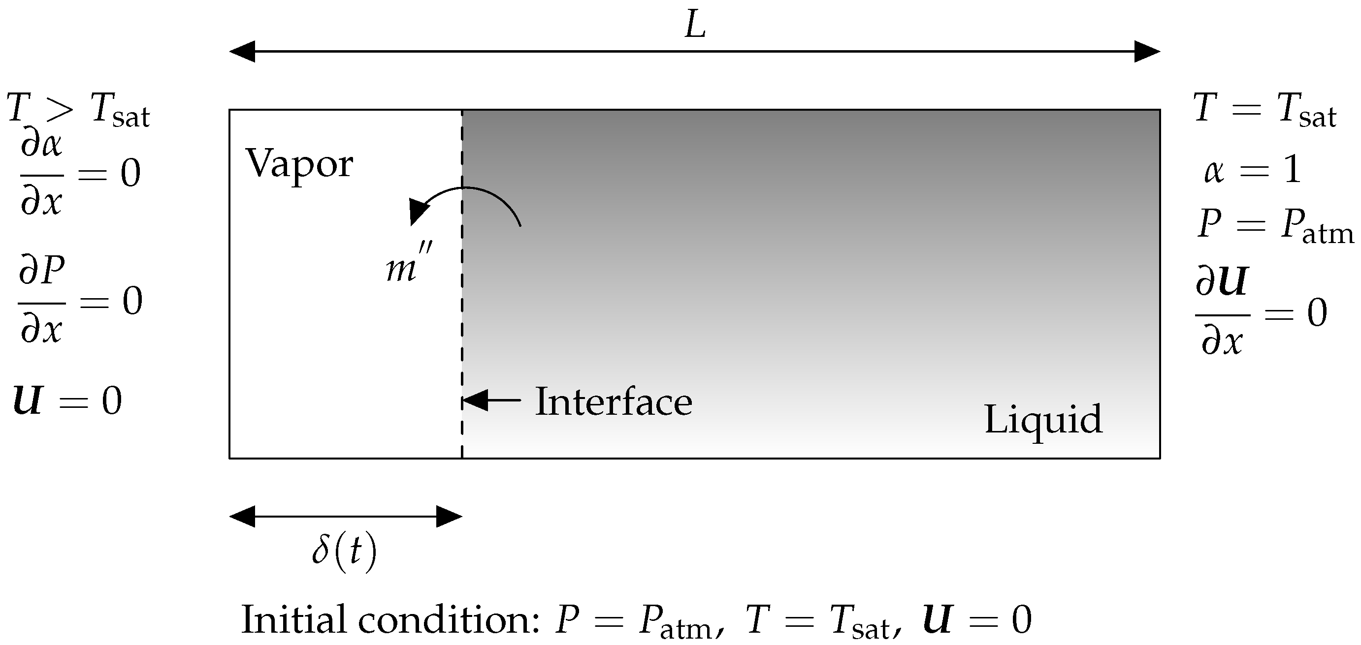
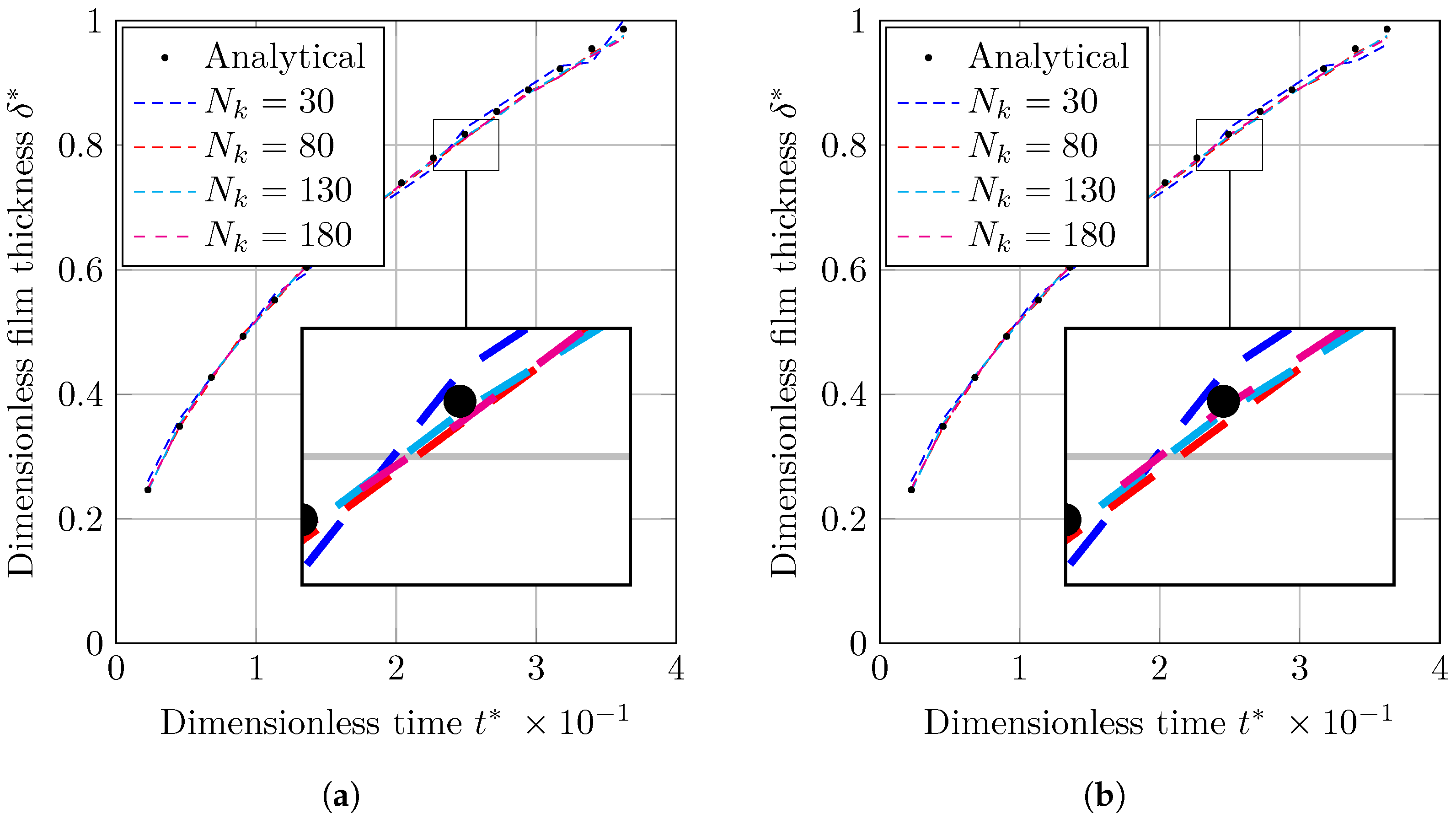
3.1. Evaporation by Heat Conduction
- The dimensionless location of the interface () through dimensionless time (), and
- Jakob number distribution (Ja) within the 1D domain to study temperature distribution.
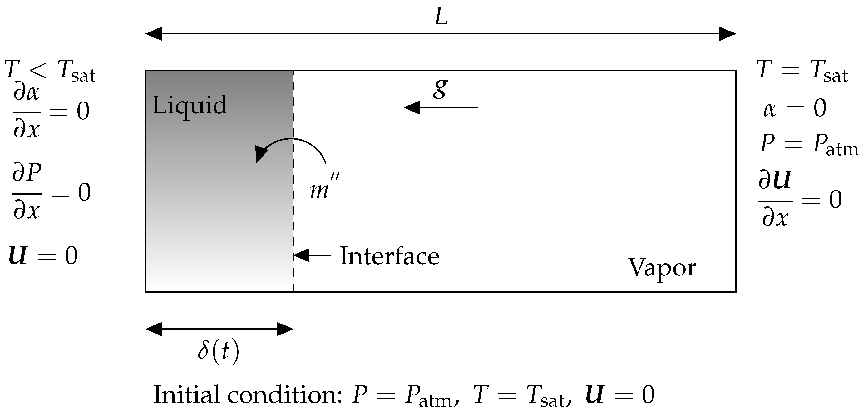
3.2. Condensation by Conduction
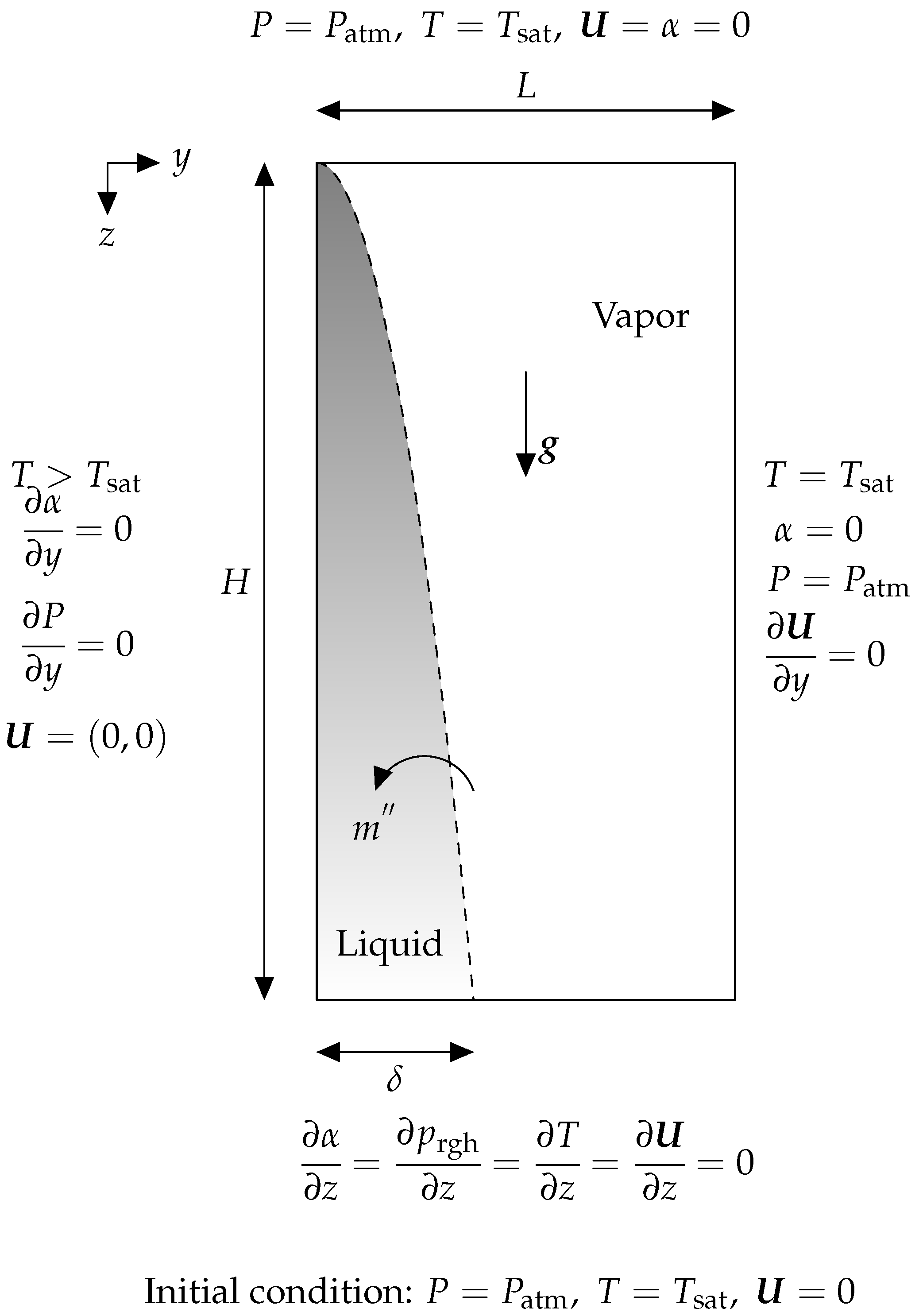
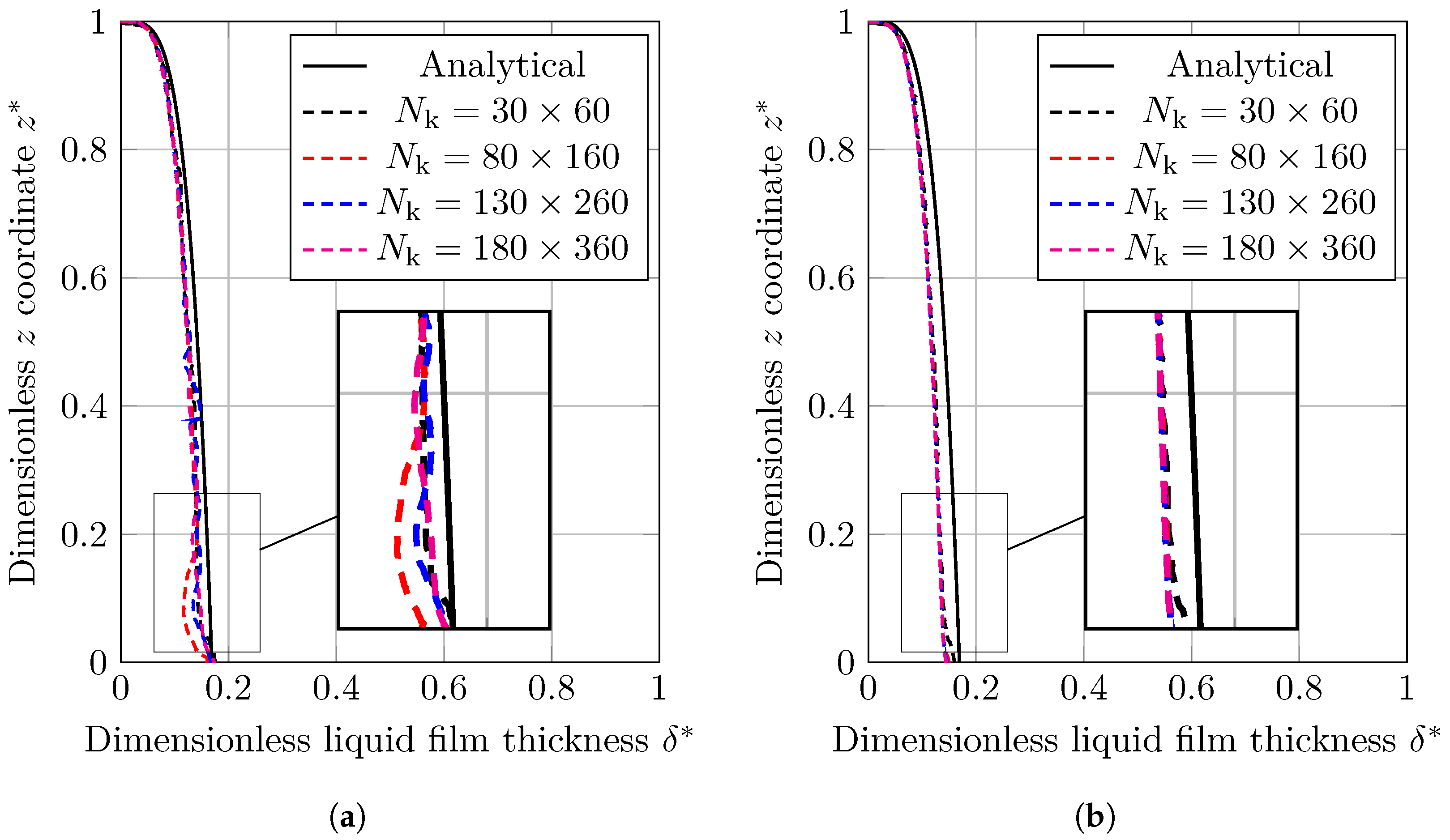
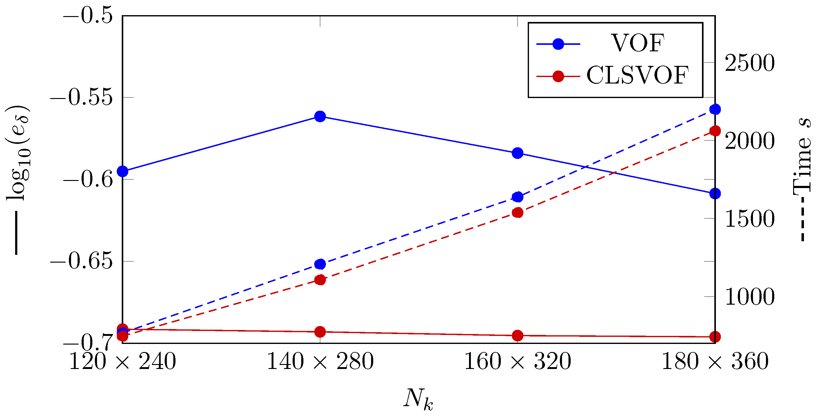
3.3. Film Condensation on a Vertical Plate
- The temperature profile across the film is linear,
- Effects of forces caused by inertia and interface shearing stress are neglected.
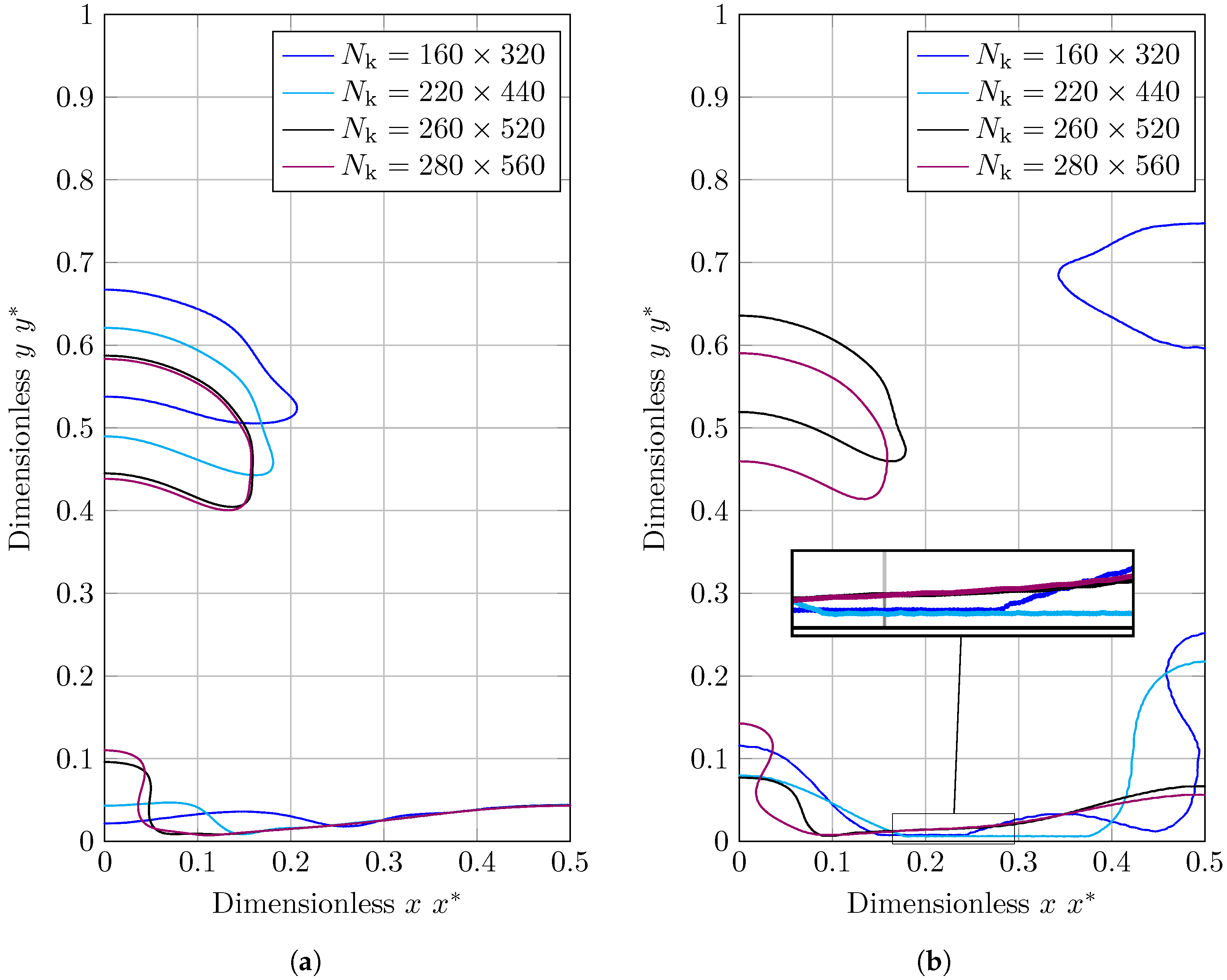
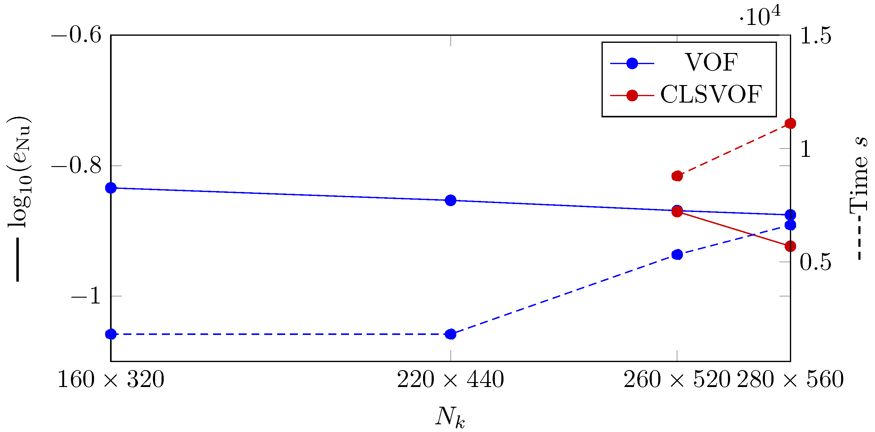
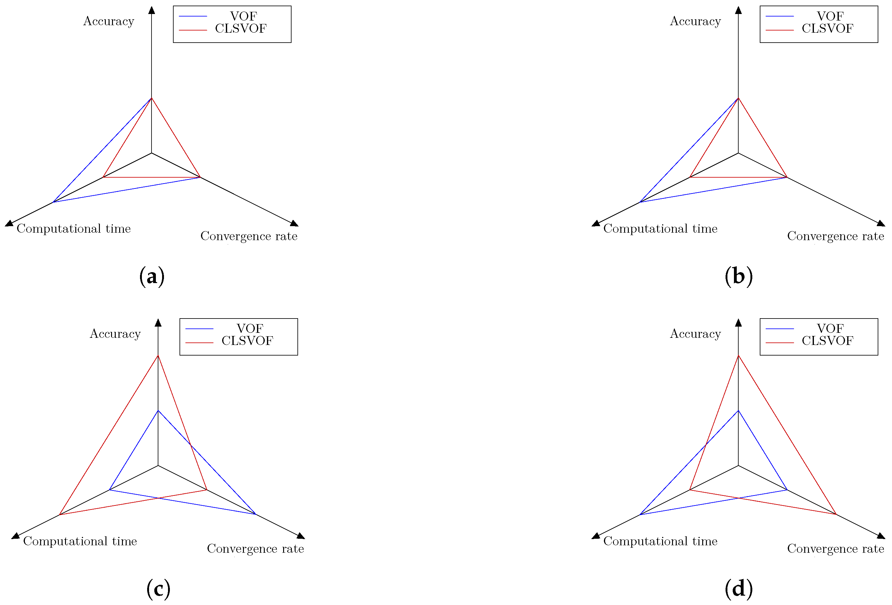
3.4. 2D Film Boiling
4. Conclusions
Author Contributions
Funding
Institutional Review Board Statement
Informed Consent Statement
Data Availability Statement
Acknowledgments
Conflicts of Interest
Nomenclature
| Volume of Fluid | |
| t | Time |
| U | Velocity |
| p | Pressure |
| Gravitational acceleration | |
| Surface tension forces | |
| m | Transferred mass |
| T | Temperature |
| c | Specific heat |
| k | Thermal conductivity |
| R | Universal gas constant |
| h | Latent heat |
| M | Molecular weight |
| V | Volume of the cell |
| Compressive factor | |
| Surface vector | |
| N | Number |
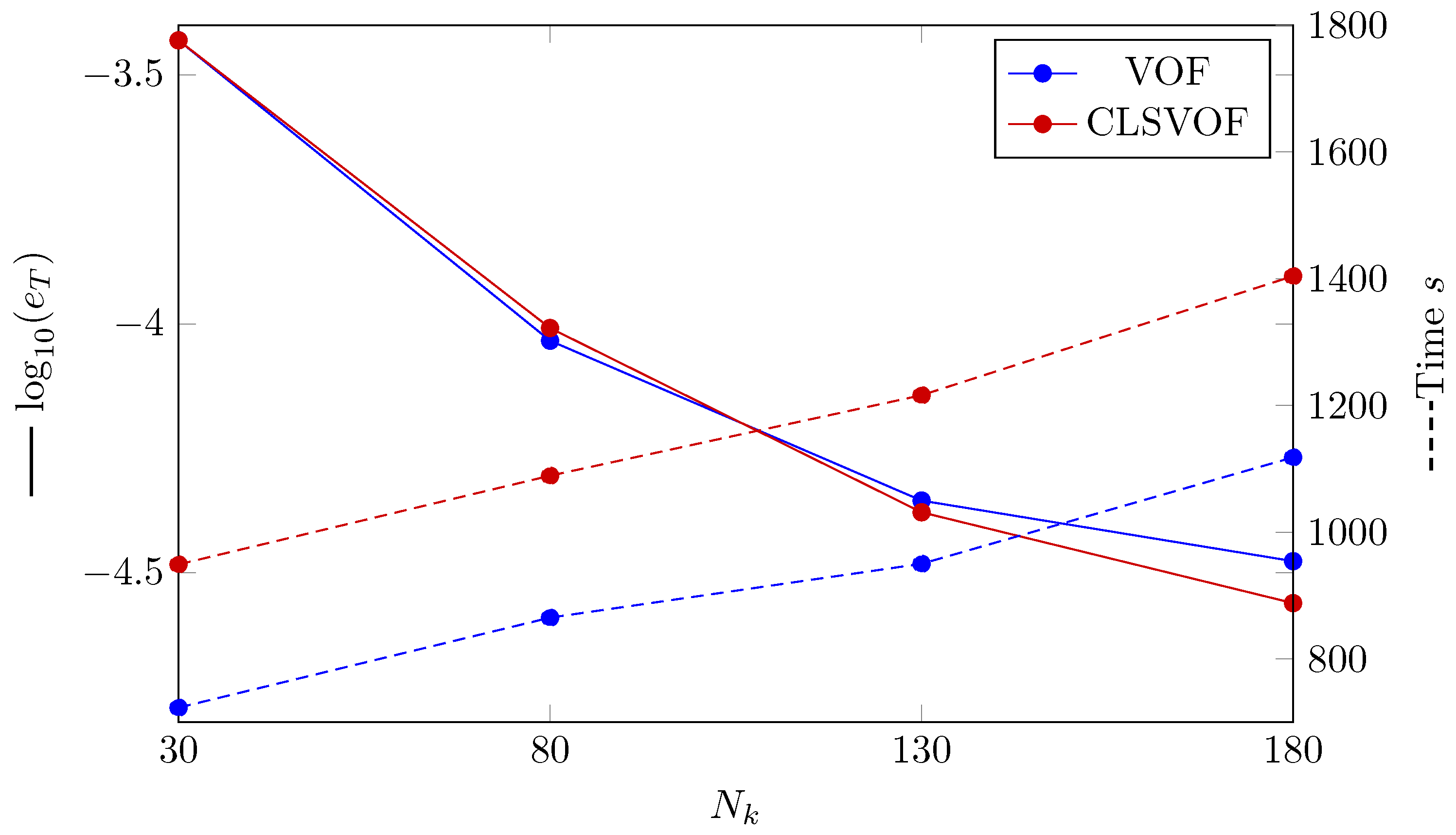
| e | error |
| R | convergence rate |
| Capillary number | |
| Jakob number | |
| Nusselt number | |
| Laplace number | |
| Dimensionless pressure coefficient | |
| Density | |
| Deviatoric viscous stress tensor | |
| Evaporation coefficient | |
| Dynamic viscosity | |
| Interface curvature | |
| p | constant pressure |
| liquid | |
| vapor | |
| saturation | |
| supersaturation | |
| subsaturation | |
| without the hydrostatic pressure | |
| total | |
| mixture | |
| compressive | |
| volume fraction | |
| capillary | |
| cell face | |
| nodes in the domain | |
| numerical results | |
| analytical results | |
| film thickness | |
| * | dimensionless |
| flux rate |
References
- Alrbee, K.; Muzychka, Y.S.; Duan, X. Heat Transfer enhancement in laminar Graetz and Taylor Flows using nanofluids. In Proceedings of the International Conference on Nanochannels, Microchannels, and Minichannels, Dubrovnik, Croatia, 10–13 June 2018; Volume 51197, p. V001T02A021. [Google Scholar]
- Sarafraz, M.M.; Tlili, I.; Tian, Z.; Khan, A.R.; Safaei, M.R. Thermal analysis and thermo-hydraulic characteristics of zirconia–water nanofluid under a convective boiling regime. J. Therm. Anal. Calorim. 2020, 139, 2413–2422. [Google Scholar] [CrossRef]
- Sujun, D.; Jiang, H.; Yongqi, X.I.E.; Xiaoming, W.; Zhongliang, H.U.; Jun, W. Experimental investigation on boiling heat transfer characteristics of Al2O3-water nanofluids in swirl microchannels subjected to an acceleration force. Chin. J. Aeronaut. 2019, 32, 1136–1144. [Google Scholar]
- Choi, S.U.S.; Eastman, J.A. Enhancing Thermal Conductivity of Fluids with Nanoparticles; Technical Report; Argonne National Lab. (ANL): Argonne, IL, USA, 1995. [Google Scholar]
- Alarifi, I.M.; Alkouh, A.B.; Ali, V.; Nguyen, H.M.; Asadi, A. On the rheological properties of MWCNT-TiO2/oil hybrid nanofluid: An experimental investigation on the effects of shear rate, temperature, and solid concentration of nanoparticles. Powder Technol. 2019, 355, 157–162. [Google Scholar] [CrossRef]
- Siahmargoi, M.; Rahbar, N.; Kargarsharifabad, H.; Sadati, S.E.; Asadi, A. An Experimental Study on the Performance Evaluation and Thermodynamic Modeling of a Thermoelectric Cooler Combined with Two Heatsinks. Sci. Rep. 2019, 9, 20336. [Google Scholar] [CrossRef] [PubMed] [Green Version]
- Lyu, Z.; Asadi, A.; Alarifi, I.M.; Ali, V.; Foong, L.K. Thermal and Fluid Dynamics Performance of MWCNT-Water Nanofluid Based on Thermophysical Properties: An Experimental and Theoretical Study. Sci. Rep. 2020, 10, 5185. [Google Scholar] [CrossRef] [Green Version]
- Rezaei, A.; Abdollahi, H.; Derikvand, Z.; Hemmati-Sarapardeh, A.; Mosavi, A.; Nabipour, N. Insights into the effects of pore size distribution on the flowing behavior of carbonate rocks: Linking a nano-based enhanced oil recovery method to rock typing. Nanomaterials 2020, 10, 972. [Google Scholar] [CrossRef]
- Razavirad, F.; Shahrabadi, A.; Dehkordi, P.B.; Rashidi, A. Experimental pore-scale study of a novel functionalized iron-carbon nanohybrid for enhanced oil recovery (EOR). Nanomaterials 2022, 12, 103. [Google Scholar] [CrossRef]
- Ahmadi, A.A.; Arabbeiki, M.; Ali, H.M.; Goodarzi, M.; Safaei, M.R. Configuration and optimization of a minichannel using water–alumina nanofluid by non-dominated sorting genetic algorithm and response surface method. Nanomaterials 2020, 10, 901. [Google Scholar] [CrossRef]
- Tirandazi, B.; Yahyaee, A.; Kianpour, M.; Shahhosseini, S. Experimental investigation and modeling of viscosity effect on carbon dioxide absorption using sodium hydroxide. J. Environ. Chem. Eng. 2017, 5, 2597. [Google Scholar] [CrossRef]
- Jamei, M.; Olumegbon, I.A.; Karbasi, M.; Ahmadianfar, I.; Asadi, A.; Mosharaf-Dehkordi, M. On the Thermal Conductivity Assessment of Oil-Based Hybrid Nanofluids using Extended Kalman Filter integrated with feed-forward neural network. Int. J. Heat Mass Transf. 2021, 172, 121159. [Google Scholar] [CrossRef]
- Asadi, A.; Bakhtiyari, A.N.; Alarifi, I.M. Predictability evaluation of support vector regression methods for thermophysical properties, heat transfer performance, and pumping power estimation of MWCNT/ZnO–engine oil hybrid nanofluid. Eng. Comput. 2021, 37, 3813–3823. [Google Scholar] [CrossRef]
- Jamei, M.; Karbasi, M.; Mosharaf-Dehkordi, M.; Adewale Olumegbon, I.; Abualigah, L.; Said, Z.; Asadi, A. Estimating the density of hybrid nanofluids for thermal energy application: Application of non-parametric and evolutionary polynomial regression data-intelligent techniques. Meas. J. Int. Meas. Confed. 2022, 189, 110524. [Google Scholar] [CrossRef]
- Rashidi, M.M.; Sadri, M.; Sheremet, M.A. Numerical simulation of hybrid nanofluid mixed convection in a lid-driven square cavity with magnetic field using high-order compact scheme. Nanomaterials 2021, 11, 2250. [Google Scholar] [CrossRef] [PubMed]
- Sadabadi, H.; Nezhad, A.S. Nanofluids for performance improvement of heavy machinery journal bearings: A simulation study. Nanomaterials 2020, 10, 2120. [Google Scholar] [CrossRef]
- Al-Yaari, A.; Ching, D.L.C.; Sakidin, H.; Muthuvalu, M.S.; Zafar, M.; Alyousifi, Y.; Saeed, A.A.H.; Bilad, M.R. Thermophysical Properties of Nanofluid in Two-Phase Fluid Flow through a Porous Rectangular Medium for Enhanced Oil Recovery. Nanomaterials 2022, 12, 1011. [Google Scholar] [CrossRef]
- Gul, T.; Qadeer, A.; Alghamdi, W.; Saeed, A.; Mukhtar, S.; Jawad, M. Irreversibility analysis of the couple stress hybrid nanofluid flow under the effect of electromagnetic field. Int. J. Numer. Methods Heat Fluid Flow 2021, 32, 642–659. [Google Scholar] [CrossRef]
- Yahyaee, A.; Bahman, A.S.; Sørensen, H. A Benchmark Evaluation of the isoAdvection Interface Description Method for Thermally–Driven Phase Change Simulation. Nanomaterials 2022, 12, 1665. [Google Scholar] [CrossRef]
- Nujukambari, A.Y.; Bahman, A.S.; Hærvig, J.; Sørensen, H. A Review: New Designs of Heat Sinks for Flow Boiling Cooling. In Proceedings of the 25th International Workshop on Thermal Investigations of ICs and Systems (THERMINIC), Lecco, Italy, 25–27 September 2019; pp. 1–6. [Google Scholar]
- Hadavand, M.; Yousefzadeh, S.; Akbari, O.A.; Pourfattah, F.; Nguyen, H.M.; Asadi, A. A numerical investigation on the effects of mixed convection of Ag-water nanofluid inside a sim-circular lid-driven cavity on the temperature of an electronic silicon chip. Appl. Therm. Eng. 2019, 162, 114298. [Google Scholar] [CrossRef]
- Yahyaee, A.; Bahman, A.S.; Blaabjerg, F. A Modification of Offset Strip Fin Heatsink with High-Performance Cooling for IGBT Modules. Appl. Sci. 2020, 10, 1112. [Google Scholar] [CrossRef] [Green Version]
- Hirt, C.W.; Nichols, B.D. Volume of fluid (VOF) method for the dynamics of free boundaries. J. Comput. Phys. 1981, 39, 201–225. [Google Scholar] [CrossRef]
- Omar, S. Development of a Hyperbolic Equation Solver and the Improvement of the School of Engineering. Ph.D. Thesis, Cardiff University, Cardiff, UK, 2018. [Google Scholar]
- Soleimani, A.; Sattari, A.; Hanafizadeh, P. Thermal analysis of a microchannel heat sink cooled by two-phase flow boiling of Al2O3 HFE-7100 nanofluid. Therm. Sci. Eng. Prog. 2020, 20, 100693. [Google Scholar] [CrossRef]
- Zhang, J.; Li, S.; Wang, X.; Sundén, B.; Wu, Z. Numerical studies of gas-liquid Taylor flows in vertical capillaries using CuO/water nanofluids. Int. Commun. Heat Mass Transf. 2020, 116, 104665. [Google Scholar] [CrossRef]
- Rabiee, R.; Désilets, M.; Proulx, P.; Ariana, M.; Julien, M. Determination of condensation heat transfer inside a horizontal smooth tube. Int. J. Heat Mass Transf. 2018, 124, 816–828. [Google Scholar] [CrossRef]
- Yahyaee, A.; Hærvig, J.; Bahman, A.S.; Sørensen, H. Numerical Simulation of Boiling in a Cavity. In Proceedings of the 26th International Workshop on Thermal Investigations of ICs and Systems (THERMINIC), Berlin, Germany, 23–25 September 2020; pp. 1–5. [Google Scholar]
- Abedini, E.; Zarei, T.; Rajabnia, H.; Kalbasi, R.; Afrand, M. Numerical investigation of vapor volume fraction in subcooled flow boiling of a nanofluid. J. Mol. Liq. 2017, 238, 281–289. [Google Scholar] [CrossRef]
- Osher, S.; Sethian, J.A. Fronts propagating with curvature-dependent speed: Algorithms based on Hamilton-Jacobi formulations. J. Comput. Phys. 1988, 79, 12–49. [Google Scholar] [CrossRef] [Green Version]
- Dhir, V.K.; Purohit, G.P. Subcooled film-boiling heat transfer from spheres. Nucl. Eng. Des. 1978, 47, 49–66. [Google Scholar] [CrossRef]
- Dhir, V.K. Boiling heat transfer. Annu. Rev. Fluid Mech. 1998, 30, 365–401. [Google Scholar] [CrossRef]
- Dhir, V.K. Numerical simulations of pool-boiling heat transfer. AIChE J. 2001, 47, 813–834. [Google Scholar] [CrossRef]
- Dhir, V.K.; Warrier, G.R.; Aktinol, E. Numerical Simulation of Pool Boiling: A Review. J. Heat Transf. 2013, 135, 061502. [Google Scholar] [CrossRef]
- Gibou, F.; Chen, L.; Nguyen, D.; Banerjee, S. A level set based sharp interface method for the multiphase incompressible Navier–Stokes equations with phase change. J. Comput. Phys. 2007, 222, 536–555. [Google Scholar] [CrossRef]
- Tanguy, S.; Ménard, T.; Berlemont, A. A level set method for vaporizing two-phase flows. J. Comput. Phys. 2007, 221, 837–853. [Google Scholar] [CrossRef]
- Sato, Y.; Ničeno, B. A sharp-interface phase change model for a mass-conservative interface tracking method. J. Comput. Phys. 2013, 249, 127–161. [Google Scholar] [CrossRef]
- Sussman, M.; Puckett, E.G. A coupled level set and volume-of-fluid method for computing 3D and axisymmetric incompressible two-phase flows. J. Comput. Phys. 2000, 162, 301–337. [Google Scholar] [CrossRef] [Green Version]
- Yu, C.H.; Wen, H.L.; Gu, Z.H.; An, R.D. Numerical simulation of dam-break flow impacting a stationary obstacle by a CLSVOF/IB method. Commun. Nonlinear Sci. Numer. Simul. 2019, 79, 104934. [Google Scholar] [CrossRef]
- Bahreini, M.; Derakhshandeh, J.F.; Ramiar, A.; Dabirian, E. Numerical study on multiple bubbles condensation in subcooled boiling flow based on CLSVOF method. Int. J. Therm. Sci. 2021, 170, 107121. [Google Scholar] [CrossRef]
- Chen, B.; Wang, B.; Mao, F.; Tian, R.; Lu, C. Analysis of liquid droplet impacting on liquid film by CLSVOF. Ann. Nucl. Energy 2020, 143, 107468. [Google Scholar] [CrossRef]
- Nemati, H.; Breugem, W.P.; Kwakkel, M.; Jan Boersma, B. Direct numerical simulation of turbulent bubbly down flow using an efficient CLSVOF method. Int. J. Multiph. Flow 2021, 135, 103500. [Google Scholar] [CrossRef]
- Tanasawa, I. Advances in condensation heat transfer. In Advances in Heat Transfer; Elsevier: Amsterdam, The Netherlands, 1991; Volume 21, pp. 55–139. [Google Scholar]
- Pak, B.C.; Cho, Y.I. Hydrodynamic and heat transfer study of dispersed fluids with submicron metallic oxide particles. Exp. Heat Transf. Int. J. 1998, 11, 151–170. [Google Scholar] [CrossRef]
- Hamilton, R.L.; Crosser, O.K. Thermal conductivity of heterogeneous two-component systems. Ind. Eng. Chem. Fundam. 1962, 1, 187–191. [Google Scholar] [CrossRef]
- Xuan, Y.; Roetzel, W. Conceptions for heat transfer correlation of nanofluids. Int. J. Heat Mass Transf. 2000, 43, 3701–3707. [Google Scholar] [CrossRef]
- Zhu, D.S.; Wu, S.Y.; Wang, N. Surface tension and viscosity of aluminum oxide nanofluids. AIP Conf. Proc. 2010, 1207, 460–464. [Google Scholar]
- Samkhaniani, N.; Ansari, M.R. Numerical simulation of bubble condensation using CF-VOF. Prog. Nucl. Energy 2016, 89, 120–131. [Google Scholar] [CrossRef]
- Shin, S.; Choi, B. Numerical simulation of a rising bubble with phase change. Appl. Therm. Eng. 2016, 100, 256–266. [Google Scholar] [CrossRef]
- Rajkotwala, A.H.; Panda, A.; Peters, E.A.; Baltussen, M.W.; van der Geld, C.W.; Kuerten, J.G.; Kuipers, J.A. A critical comparison of smooth and sharp interface methods for phase transition. Int. J. Multiph. Flow 2019, 120, 103093. [Google Scholar] [CrossRef]
- Nusselt, W. Die oberflachenkondensation des wasserdamphes. VDI-Zs 1916, 60, 541. [Google Scholar]
- Samkhaniani, N.; Ansari, M.R. The evaluation of the diffuse interface method for phase change simulations using OpenFOAM. Heat Transf.—Asian Res. 2017, 46, 1173–1203. [Google Scholar] [CrossRef]
- Berenson, P.J. Film-boiling heat transfer from a horizontal surface. J. Heat Transf. 1961, 83, 351–356. [Google Scholar] [CrossRef]


| Publication | Remarks |
|---|---|
| Soleimani et al. [25] | The VOF method is used to model subcooled flow boiling of HFE-7100 in a microchannel heat sink with variable concentrations of alumina nanoparticles. |
| Zhang et al. [26] | In a tiny tube, the VOF approach is used to quantitatively investigate the heat transfer and pressure drop properties of gas–liquid Taylor flows. CuO/water nanofluid was the liquid, while nitrogen was the gas. |
| Rabiee et al. [27] | flow condensation inside a smooth horizontal tube was simulated. Moreover, the effect of some parameters such as mass flux, tube hydraulic diameter, vapor quality and difference between the wall and saturation temperature on the heat transfer coefficient were investigated. |
| Yahyaee et al. [28] | This article simulates the development of bubbles and their escape from a superheated horizontal surface. A cylindrical hollow initiates the bubble nucleation process. The simulation will be carried out utilizing VOF using a new OpenFOAM-based two-phase solver. |
| Abedini et al. [29] | The VOF method are used to explore the subcooled boiling of Alumina-water nanofluid in both vertical concentric annulus and vertical tube. There is a comparison of the inlet vapor volume fraction fluctuation at various nanoparticles concentrations. |
| Terms | Schemes |
|---|---|
| Temporal term | Backward |
| Convective term in momentum equation | vanLeerV |
| Convective term in energy equation | vanLeer |
| Compression velocity term in momentum equation | interfaceCompression |
| Diffusion term in momentum equation | Gauss Linear corrected |
| Viscous term in momentum equation | Gauss Linear |
| Dimension | Base Fluid | Nanoparticles | Vapor | |
|---|---|---|---|---|
| Thermal conductivity, k | 0.648 | 36 | 0.03643 | |
| Density, | 645 | 3600 | 5.1450 | |
| Viscosity, | Pa s | |||
| Specific heat capacity | 2.794 | 0.765 | 2.687 | |
| Latent Heat, h | 762.52 | 2777.1 | ||
| Surface tension, | 0.045417 |
| Dimension | Base Fluid | Nanoparticles | Vapor | |
|---|---|---|---|---|
| Thermal conductivity, | 0.531 | 36 | 0.538 | |
| Density, | 370.4 | 3600 | 242.7 | |
| Viscosity, | Pa s | |||
| Specific heat capacity | 239 | 0.765 | 352 | |
| Latent Heat, h | 1963.5 | 2240 | ||
| Surface tension, |
| L | Length of domain | 0.5 L |
| H | Height of domain | 3 L |
| Thickness of condensed film at | 0.01 L |
Publisher’s Note: MDPI stays neutral with regard to jurisdictional claims in published maps and institutional affiliations. |
© 2022 by the authors. Licensee MDPI, Basel, Switzerland. This article is an open access article distributed under the terms and conditions of the Creative Commons Attribution (CC BY) license (https://creativecommons.org/licenses/by/4.0/).
Share and Cite
Yahyaee, A.; Bahman, A.S.; Olesen, K.; Sørensen, H. Level-Set Interface Description Approach for Thermal Phase Change of Nanofluids. Nanomaterials 2022, 12, 2228. https://doi.org/10.3390/nano12132228
Yahyaee A, Bahman AS, Olesen K, Sørensen H. Level-Set Interface Description Approach for Thermal Phase Change of Nanofluids. Nanomaterials. 2022; 12(13):2228. https://doi.org/10.3390/nano12132228
Chicago/Turabian StyleYahyaee, Ali, Amir Sajjad Bahman, Klaus Olesen, and Henrik Sørensen. 2022. "Level-Set Interface Description Approach for Thermal Phase Change of Nanofluids" Nanomaterials 12, no. 13: 2228. https://doi.org/10.3390/nano12132228
APA StyleYahyaee, A., Bahman, A. S., Olesen, K., & Sørensen, H. (2022). Level-Set Interface Description Approach for Thermal Phase Change of Nanofluids. Nanomaterials, 12(13), 2228. https://doi.org/10.3390/nano12132228