Abstract
After nearly thirty years of concerted effort by many investigators, the cause or causes of the secular gains in IQ test scores, known as the Flynn effect, remain elusive. In this target article, I offer six suggestions as to how we might proceed in our efforts to solve this intractable mystery. The suggestions are as follows: (1) compare parents to children; (2) consider other traits and conditions; (3) compare siblings; (4) conduct more and better intervention programs; (5) use subtest profile data in context; and (6) quantify the potential contribution of heterosis. This last section contains new simulations of the process of heterosis, which provide a plausible scenario whereby rapid secular changes in multiple genetically influenced traits are possible. If there is any theme to the present paper, it is that future study designs should be simpler and more highly focused, coordinating multiple studies on single populations.
1. Introduction
It has been nearly thirty years since James Flynn brought widespread attention to the occurrence of rapid gains in IQ test scores [1,2]. However, in honestly assessing the situation today one would have to conclude that we are not much closer to identifying the cause than we were three decades ago. At present, there is no consensus that any portion of the trend can definitively be ascribed to any specific factor [3]. Today few members of the scientific community, much less the general public, are even aware that IQ scores have risen. However, a reasonable case can be made that identifying the cause of the Flynn effect is the most important question facing science today. This is because a certain level of psychometric intelligence is necessary, though not sufficient, to perform every job done in a modern industrialized society [4,5]; and it has been the development and continued maintenance of these societies that has lifted so much of humanity out of poverty, drudgery, illness, and early death [6]. Higher mean IQ enables a society to improve its overall material condition.
A convenient, though imperfect, proxy for the greater productivity of high IQ individuals is income. A positive association between IQ and income shows up at every conceivable level of analysis. Among nations, those with higher IQ tend to have higher per capita income [7]. Within nations, those regions and ethnic groups with higher IQ have higher income (e.g., [8]). Even within families, the higher IQ sibling tends to have higher income [9]. Importantly for the present discussion, the IQ-income relationship also appears to hold up within populations over time. When IQ scores rise, per capita income tends to increase as well [10,11].
Identifying the cause of the IQ trend would offer us the real prospect of alleviating poverty worldwide. If the cause of the Flynn effect is found to be manipulable, we might then have the capacity to significantly boost worldwide IQ. Income gains would likely follow, as they have in all populations where scores have thus far risen. Even if the Flynn effect is not easily manipulated, simply understanding the problem correctly might provide a rationale for measures that alleviate want in the absence of intelligence gains. Although a correct understanding of things does not guarantee a good outcome, it inevitably increases the probability of solving the problems we face.
Despite its enormous potential importance, basic questions related to the IQ trend remain unanswered. In this target article, I offer six suggestions for improving our research efforts. If they have any theme, it is that future research needs to be simpler and more highly focused. While focusing on methodology, the specific prescriptions offered here are all accompanied by a discussion of the underlying theoretical rationale and assumptions upon which they are based. The six suggestions for future research are as follows: (1) Compare parents to children; (2) consider trends in other traits; (3) compare siblings; (4) improve intervention studies; (5) use IQ subtest studies in context, and (6) quantify the potential effect of heterosis.
As this issue focuses on methodology, it is not the place to weigh the strengths of different hypotheses. In the interest of full disclosure, however, I have argued for more than a decade that the most plausible cause of the Flynn effect is the genetic factor heterosis [10,12], (however, see [13]). For the record, I still believe heterosis is the only factor capable of explaining all relevant findings, including the consistently high heritability of IQ, the lack of shared family environmental effects, the so-called “twin paradox,” the occurrence of trends in many other traits and conditions, the steady pace of the changes, the appearance of several of the trends in very young children, the limited impact of intervention efforts, the lack of lasting effects due to environmental insults, evolutionary implications, the magnitude of the changes, and other findings. The last suggestion in this paper is the only one to deal directly with heterosis, but my preference for it can be seen in the discussion of some of the other research proposals. When an example is needed to make a point, I usually turn to findings related to heterosis as this is the area I am most familiar with.
2. Suggestion 1: Compare Parents to Children
Decades ago, data from the Fels Longitudinal Study suggested that U.S. secular gains in height had ceased. The Fels data, however, allowed for the comparison of parents to their own children, which showed that adult children were 3 cm taller, on average, than their parents when measured at the same age [14]. In this case, the discrepancy was the result of recruitment of new families who were shorter, as well as differential fertility. However, the broader lesson is that cohort comparisons will capture the effects of a somewhat different set of factors than parent-child comparisons. Therefore, supplementing cohort studies with intergenerational studies has the potential to shed light on the factors that affect traits over time.
Two factors that will affect cohort comparisons, but not parent-child comparisons, are migration and differential fertility. Migration here refers to the introduction or removal of families, who are now represented in one cohort but not the other. Differential fertility occurs when parents who are above or below average in IQ have more children, or have them at a younger age. For example, if a population is receiving lower-IQ immigrants, and lower-IQ individuals are having more children, any negative effects of these two factors would be offsetting IQ gains which children might be making over their parents (or exacerbating IQ losses). One would now expect a discrepancy between cohort comparisons and parent-child comparisons that would require explanation. Although seemingly straightforward, comparing parents to children is actually fraught with methodological pitfalls. I list below a few of these and describe a specific study design that I believe would represent a good starting point for parent-child IQ comparisons.
One difficulty results from regression to the mean. High IQ parents have children who tend to score lower than themselves, while children of low IQ parents tend to outscore their parents [15]. In effect, then, the question is not whether children score higher than their parents, but whether they are regressing to a higher mean than that of their parents’ generation. An unrepresentative sample of parents will result in an apparent but spurious parent-child difference. Importantly, the parents must be representative of the entire parental cohort, not merely representative of those who had children. Finding such a sample of parents is difficult because parents can be members of different cohorts, and cohort IQ is often changing. Also, IQ tends to display assortative mating [16], which can vary in different IQ ranges and over time.
A second set of problems arises from the fact that parents do not all wait until the same age to have their children, and have multiple children. Imagine two siblings with identical test performance, both scoring six points higher than their parents. The older sibling is born to the parents when they are 20 and so contribute to secular IQ gains of three points per decade. The younger sibling is born when the parents are 30, contributing to a gain of two points per decade. For this reason, incorporating parental age is essential when comparing parent-child studies to cohort studies.
Lastly, there is the possibility of differences among siblings from such things as birth order effects, parental age effects, and secular changes in the non-shared environment. Recently, in Norwegian military data, Sundet et al. found that later-born siblings tended to be lower in IQ than earlier-born siblings, but that the deficit varied as a function of age difference and the rate/direction of cohort changes. In times of rising IQ, the deficit narrowed with increasing age difference, while in times of declining IQ, it widened [17]. Any study should, therefore, try to break down intergenerational IQ changes into those caused by children with different characteristics, such as birth order or parental age.
Military data has several advantages for comparing parents to children. In countries with compulsory service, thousands of father-son pairs were administered the same test at approximately the same age. Importantly, this same military data allows for the comparison of cohorts, against which to gauge comparisons between fathers and sons. In addition, with data from an entire cohort, one can more easily choose a sample of fathers that is representative of an entire cohort. Although military data contain no measure of mother’s IQ, this can likely be estimated based on fathers’ IQ and other family IQ studies. At least two countries, Norway and Sweden, have military IQ data that allow father-son pairs to be identified [18,19], and others likely exist.
In a situation of nearly complete ignorance, such as we are in with regard to the Flynn effect, a simple, highly focused study design may be preferable to a complex regression analysis involving multiple factors that may or may not be affecting IQ. In this spirit, the study design proposed here would start with only those men who score at or near the mode from one particular birth cohort, based on military data; these are the fathers. I suggest the mode here because military data can exclude ten percent or more of men. The fact that those excluded are likely not representative makes the mode a somewhat better measure of central tendency. The mode, however, can also be problematic, as when IQ is recorded in coarse units such as stanine scores. The point is that the measure of central tendency used requires consideration. We want the measure of central tendency of the parents, to which we would expect the children to regress in a population at equilibrium (i.e., no secular changes in any factors influencing IQ, no migration, no differential fertility, etc.).
Once the sample of fathers is identified, one would then identify all of their sons for whom test data are available. One would have to ensure that the test norming procedures have remained the same over time, or adjust scores for changes. Initially, one could simply take the average of the sons’ scores and compare it to the fathers’ score. The sons could then be subdivided according to factors such as birth order, year of birth, year of testing, and parental age at birth to determine how children in different categories are contributing to intergenerational differences. The study could then be expanded to fathers above and below the “mode” to see if sons are regressing to a different “mean” than that of the fathers’ generation (considering the above discussion of the appropriate measure of central tendency). While there are additional potential biases to consider, the above type of analysis would represent a good start to parent-child comparisons for traits such as IQ and height.
There are certain cases where it would be particularly interesting to compare parents to children. For example, in the aforementioned study from Norway, there was one period in which scores were rising (those born 1950–1956), and another where scores were falling (born 1976–1983). Because these periods are separated by about 25 years, many of the men in the earlier group were the fathers of men in the latter group. This raises the possibility that the performance of cohorts was declining during a period when the IQ of the typical father was rising. If the rate of gains in the fathers was about equal to the rate of decline in the sons, then the amount of decline to be explained would arguably be twice as large as that measured by the cohort decline alone. While this is an interesting case, parent-child comparisons should be done wherever the data permit, especially given the likelihood of at least some migration and differential fertility in many populations today [20].
3. Suggestion 2: Consider Other Traits
In those places and times that IQ scores have risen, every heritable trait has changed at a rate that is on the same order of magnitude as that seen in IQ, approximately 0.2 to 0.5 standard deviations per decade. Likewise, the incidence of every heritable threshold condition has changed at a rate to be expected if an underlying normal liability distribution were shifting at a similar pace (see [10], p. 825 for examples). Of course, I cannot prove the above statement holds for every heritable trait and condition; I have intentionally risked overstating the case for broad-based secular changes in the hope of provoking a response. Commentators are invited to list traits and conditions for which there is good evidence of stasis; they may be able to name a few, but it will not be easy. In more than a decade of studying trends, I am not aware of any clear exceptions, but many examples of undeniable change [10,12]. If its heritability is greater than zero and IQ scores have risen in the population, substantial change in the trait is the rule, stasis the exception.
The above challenge has already begun generating a discussion, even before publication of this article. All three reviewers of this article raised concerns with the statement made above. One reviewer points out that “Norwegian data do not seem to support the contention that increasing height is associated with the FE in a simple manner.” I assume the reviewer is referring to slight discrepancies in the characteristics of the trends, such as gains sometimes being stronger in the upper half of the height distribution, but the bottom half of the IQ distribution. While such differences are noteworthy, they must be viewed against the backdrop of remarkable overall synchronicity of the trends across time and place, and do not represent an exception to the general “rule of thumb” that heritable traits have tended to trend together. In Norway specifically, this can be seen in in the work of Sundet et al. [21], who state that “It can be seen from Figure 3 that the mean standing height and mean GA follow each other quite closely.”.
Another reviewer pointed to studies suggesting stasis in personality traits [22,23]. However, a cursory review of the literature reveals a lively debate over whether there have been cohort effects in personality. For example, Smits et al. [24] provide evidence of cohort effects in three of the big five personality traits, as well as a summary of citations, both for and against secular change. While it may be fairly argued that the above “rule of parallel change” has not yet been solidly confirmed in the case of personality, it has clearly not yet been disconfirmed either. It is also worth noting that for most of the secular trends, initial reports of change were met with skepticism, with opinion only gradually coalescing that real change had occurred as more data came to light.
The occurrence of secular changes in other traits has several methodological implications for the study of IQ trends. For starters, wherever there is data on more than one trait or condition, its rate of change should be compared to that seen in IQ. In fact, all of the methodological suggestions proposed in this paper could be applied to trends in other traits. As discussed above, parents and children should be compared; an interesting question is whether those families that witness the largest intergenerational increases in IQ also display larger changes in other traits. As discussed below, it would be helpful to know if the trends in other traits occur among siblings within the same family, or whether different traits are correlated among siblings. It is understandable that IQ researchers might be hesitant to delve into an analysis of anthropometric traits or immunological disorders, but someone has to do it. If investigators in each field hesitate to leave their narrow domain of expertise, opportunities to explore common causes will inevitably be missed.
The occurrence of other trends is also relevant to IQ because many of them represent either direct or indirect evidence of secular change in brain physiology. The overall documented gains in height are now approaching three standard deviations in some countries [6,25]. Milestones of maturation, such as age at menarche, now occur years earlier [26,27]. It is difficult to imagine factors causing growth in the arms, legs, and torso that is so much greater and more rapid without affecting brain development. The incidence of cognitive developmental disorders, such as autism and attention-deficit/hyperactivity disorder, or ADHD, appear to be rising [28,29]. Left-handedness has risen in many places, suggesting changes in brain lateralization [30]. Even the secular rise in myopia suggests changes in brain chemistry, as it is mediated by the neurotransmitter acetylcholine [31,32]. More directly, there is evidence of changes in the dimensions of the head, face, and brain [33,34,35] (see also [12,36] for lists of additional references, and [37] for evidence of changes in very young children).
One reviewer has urged caution in suggesting that autism and ADHD are rising, pointing out that there is still dispute over whether the apparent increases in incidence might be explained by better ascertainment or changing diagnostic criteria [28,29]. However, such factors have thus far failed to account for the full magnitude of the reported changes (see e.g., [38]). While I am not advocating that these be casually dismissed, excessive caution is equally unwarranted. Many heritable traits and conditions have undergone undeniably real change, so that genuine change in the incidence of ADHD and autism should come as no surprise, especially when other trends point to change in brain physiology. The apparent rates at which these conditions have changed are in line with those expected if an underlying normal liability were shifting upward at a rate similar to other traits. In the particular case of autism, prolonged unwillingness to admit that a real increase is occurring will inevitably retard the search for possible causes. In the meantime, parents are filling in the gaps in our knowledge with their own preferred cause, vaccines, and posing serious risks to public health [39]. This makes the danger of too much caution as real as that of too little.
One trait that arguably deserves more attention than others is brain size. IQ is positively correlated with brain volume within generations [40]; however, little effort has been devoted to determining whether this also holds among generations. That is, when IQ rises, does average brain volume also increase, and vice versa? Decades ago Lynn cited evidence of increasing brain size in support of the nutrition hypothesis [36]. Storfer also identified this as an important research question and made a strong circumstantial case for the occurrence of secular gains [41]. Storfer also made a plea for the use of a longitudinal-versus-cross-sectional study design to try and get at the question ([41] p. 274, reiterated by [12] p. 71). The idea involves finding individuals whose brains were imaged years ago, and reexamining them to quantify the effect of ageing. The longitudinal effect of age could then be subtracted from the effect of age on cross-sectional studies, with the difference attributable to secular change.
Our best current estimate of the effect of age on brain volume comes from a recent review of 56 longitudinal studies by Hedman et al. [42]. They report, for example, that “between 18 and 35 years of age, possibly another wave of growth occurs or at least a period of no brain tissue loss.” Assuming no longitudinal decline in this age group means that any decline with age from a cross-sectional study is likely due to secular gain. An example of a cross-sectional study is provided by Walhovd et al., who imaged 883 individuals from Sweden, Norway, and the U.S. [43]. The most suitable age groups for comparison to the longitudinal result above are those aged 18–29 years versus those 30–39 years. In both men and women, the older group had smaller total brain volume. In women, the difference worked out to approximately 0.2 SD/decade, while in men it was 0.15 SD/decade (calculated from [43] Table 3, pp. 923–924, mean total volume of younger group minus volume of older group divided by standard deviation of older group, divided by 1.1 decades between groups, for women and men separately). The percentage difference was nearly identical in men and women, 1.6% and 1.7% in women and men, respectively, per decade.
Admittedly, the combined sample size of both age groups in the Walhovd et al. study was less than 400, and there were only 2200 subjects in the review of longitudinal studies, less in the age group considered. While total brain volume was greater in the younger group of the cross-sectional study, several specific brain regions were larger in the older group, raising the possibility of gains in the volume of some regions but declines in others. Extrapolating these results to trends involving millions over many decades is unwarranted; however, it would hardly be surprising if brain volume has increased along with IQ. In fact, it would be far more surprising if brain volume has been in stasis, as it would then be perhaps the only heritable trait that has remained unchanged.
More than anything, the above analysis demonstrates that more can be done to quantify secular changes in brain physiology. In fact, it is something that simply must be done given that so many outward manifestations of underlying brain physiology have changed. The U.S president recently announced a new multi-billion dollar initiative to fund brain research (e.g., [44]). This author can think of no better use for such funds than determining to what extent the size, structure, lateralization, growth tempo, and chemistry of the brain have changed in recent human history.
4. Suggestion 3: Compare Siblings
In quantitative genetics generally, and behavior genetics in particular, genetic and environmental influences are often confounded. Study designs are said to be “genetically informed” when they have some capacity to disentangle these effects. One such study design involves the use of non-twin siblings. This design relies mainly on the assumption that full biological siblings are “genetically comparable.” I discuss below possible exceptions to this assumption, recent results of sibling comparisons in IQ, problems with past analyses, and areas of future use of this study design. I advocate a simple exploratory study design that provides a starting point for future investigations over complex regression analyses. The use of siblings to understand the nature of the Flynn effect was discussed by Rodgers [45], as well as Mingroni [10,12]. A good general discussion of many of the issues presented below can also be found in an article by Lahey and D’Onofrio [46].
In the simple study design being advocated here, one starts with a large number of pairs of full biological siblings. One then splits up each pair according to some criterion, putting one sibling into group A and the other into group B. For example, one might put the older member of each pair into group A and the younger into group B. Lastly, one compares the two groups in some trait of interest, such as IQ, height, or visual acuity. Due to the stochastic element of sexual reproduction, any single pair of siblings will differ genetically. However, with a large enough number of pairs, the genetic differences between groups should even out; the older sibling will get more trait-increasing genes in half the pairs, the younger will get more in the other half. With enough pairs, groups A and B should have essentially the same genetic potential for the trait, so that any difference between them can reasonably be attributed to environment. By choosing pairs with different characteristics, and/or by altering the criteria by which we split up the pairs, one can gradually understand the environmental factors that cause siblings to differ, if there are any. With regard to the Flynn effect, because siblings are born at different times, one can determine if the factors responsible for cohort changes also affect siblings differently.
As the non-twin sibling design relies heavily on the assumption that siblings have an equal chance of inheriting any given parental gene, it is worth a detailed discussion of possible violations (see [46] p. 322 for a similar but not completely overlapping list of limitations). Only full biological siblings are genetically comparable, so adoptees should be excluded if possible. Half-siblings should be removed for the same reason, although their inclusion will only create bias if the non-shared parents differ in some salient way. In addition to known half-siblings, there is also the case of half-siblings resulting from incorrect assignment of parentage (e.g., [47]). The inclusion of opposite-sex sibling pairs will likely not constitute bias, as long as the male/female ratio is equal in groups A and B. Variability in age at time of testing/measuring/diagnosis need not constitute bias, as long as its distribution is approximately the same in both groups. If the sex ratio, age at testing, or other salient characteristic differs significantly between groups, pairs can be randomly removed in such a way as to make the groups comparable.
A somewhat less obvious violation of the genetic comparability assumption will occur if the phenotype of earlier born siblings affects the decision to have more children, combined with sibling regression to the mean. As an extreme example, imagine if parents waited until their first-born was old enough to be tested in IQ, and only tried to have a second child if the first one is found to have IQ above 120. Second-born children would have lower IQ due to regression to the mean. This is an unlikely source of bias in IQ studies, but might be more significant in studies of certain conditions diagnosed early in life (e.g., [48,49]). Lastly, a violation of the genetic comparability assumption will result from changes in the genetic characteristics of sperm and egg. Studies of de novo mutations suggest they increase over time, mainly with paternal age [50].
If one is willing to neglect possible violations of the genetic comparability assumption, there are some additional methodological caveats to keep in mind. The criterion on which one is splitting the pairs cannot be one that may be genetically influenced. In an IQ study, for example, it is likely okay to split the pairs according to birth order, but not according to years of education completed (see also [46] p. 320). The criteria for ascertainment of subjects must not change over time. As with parent-child comparisons, the measurement of all siblings should be carried out as uniformly as possible. For IQ, a comparison based on raw scores is preferable. Even if the norming procedure used is identical, the norming process inevitably involves some rounding up or down of actual performance, thus adding error, which can be substantial when performance is normed coarsely, as when stanine units are used. If only normed scores are available, care should be taken to ensure that the norming standard remained unchanged over time. That is, two individuals with identical test performance must always be assigned the same normed scores for purposes of the analysis.
There is a sizeable existing literature on the use of siblings to understand the sources of variance of traits such as IQ and height [19,51,52,53,54]. However, many of these use complex regression analyses, which, given their complexity, tend to involve implicit assumptions. For example, Myrskyla et al. [19] analyzed Swedish military IQ data containing a large number of brother pairs. Among other things, the authors claim to have “accounted for the IQ time trend by adjusting for year of birth.” They then proceed to make claims regarding the factors they believe are causing differences within families. However, the question of the extent to which the time trend operates within versus between families is still very much an open one; “accounting” for a time trend that is poorly understood requires one to make a questionable assumption about how it operates. In this specific case, the problem arises from the comparison of siblings, not on their raw scores, but on scores that have first been individually regressed using data on unrelated individuals. In the analysis proposed here, such regression of individual scores is strictly avoided, whether on year of birth or any other variable.
As the strict avoidance of individually regressed scores proposed here has been met with some concern by reviewers, I would like to clarify its rationale with a hypothetical example of the type of analysis I am suggesting. Suppose that cohort IQ has been rising at a rate of three points per decade. From military data, 1000 pairs of full biological brothers are identified, all of whom differ in age by 10 years. All 1000 earlier-born brothers are put into group A, all 1000 later-born ones into group B. We find that the raw scores of groups A and B have identical means and standard deviations. Now, had one first regressed individual scores on any variable, an apparent within-family difference would appear where none existed. Regressing on year of birth, for example, would induce an apparent three-point deficit in the later born brothers (10 years × 3 points/decade). Conversely, any real difference in raw scores would be masked or exaggerated by the use of regressed scores. Again, the primary advantage of sibling data is that they give us the ability to control for genetic differences. Differences between groups A and B in raw scores can reasonably be attributed to environment. Differences in regressed scores, where the regression is based on data from unrelated individuals, cannot confidently be attributed to anything without a precise understanding of all the factors causing the association between unrelated individuals, including those operating both within and between families.
Although one can be reasonably confident that sibling differences in raw scores are environmental in origin, results from any single set of pairs will likely not tell us much about the specific environmental factors at work. For this one has to try varying the criteria by which we identify and divide pairs in an exploratory manner. In the hypothetical example above, there was no difference between groups A and B, so there is nothing to explain; we have to move on to a different set of pairs (see [46], p. 321 for similar zero results in a different context). If, however, a difference is observed, one could examine different pairs or particular subsets of the pairs to try to understand the cause of the difference. For example, one might compare the 500 pairs who are closest in birth order to the 500 who are farthest apart in birth order. One could divide the 1000 pairs according to maternal age at the time of the birth of the older brother, or age at testing. One could look at sibling pairs born five years, or 15 years, apart, and so forth. The results of each separate analysis should suggest where to explore next. By comparing the results from different pairings, each genetically informed, one should gradually be able to figure out what environmental factors are most likely causing differences among siblings, if there are any. If differences are consistently found, one can eventually attempt to regress the differences between the siblings’ raw scores on the difference between the siblings in the proposed causal factor (see [17], Figures 2 and 3).
The most promising sibling study conducted along the lines of that being proposed here is the aforementioned Norwegian study by Sundet et al. [17]. Again, they found that later-born siblings were generally lower in IQ than their earlier-born siblings, but that this deficit varied, depending on the rate and direction of cohort changes, as well as on the siblings’ age difference. When cohort scores were rising, the later-born siblings seemed to benefit from the improving environment; when scores were falling, they seemed to suffer more due to the deteriorating environment. This suggests two types of environmental factors. First, there is a birth order effect of approximately two IQ points favoring the earlier-born sibling. This effect appears to be independent of age difference and consistent over many decades, persisting up to those tested circa 2000. Secondly, there are the environmental factors that are causing cohort changes, and that are also affecting siblings within the same family differently. The study had the advantage of large sample sizes. Adoptees and half siblings appear to have been included, although this is not likely to have altered the results much. Importantly, some care was taken to ensure that the norming procedures, from the raw scores to subtest normed scores, and from subtest scores to general ability stanine scores, were done according to consistent standards, or adjusted for changes when necessary. Increased de novo mutations seem an unlikely cause of the birth order effect, as it appears to be independent of sibling age difference.
The Norwegian findings are important for several reasons. If widely replicated, the finding would allow us to rule out genetic factors, such as heterosis as the primary cause of IQ gains. Likewise, we could rule out homosis (the opposite of heterosis), dysgenic fertility, and immigration as primary causes of the recent IQ declines in some countries, as none of these would be expected to operate within families [20,55]. We could also rule out any environmental factor that would not be expected to change over time within families. The study provides strong evidence of a birth order effect, but suggests that one must first account for the effect of secular changes in the non-shared environment to quantify it. Previous twin and adoption studies have generally failed to identify specific environmental factors of any great potency [56]. As such, the findings from Norway represent what may be the first genetically informed study of IQ to show substantial environmental effects, particularly in adulthood. For these and other reasons, the result cries out for follow-up, both to look at the Norwegian data in more detail, as well as replicate the results in other data.
There are innumerable ways in which the Norwegian data could be further analyzed in the exploratory manner described above. For starters, there is no reason to restrict analysis to pairs in the three time periods considered; all pairs could be considered simultaneously. To do this, one would start with the IQ of the earlier-born of each pair, add or subtract the difference between the brothers’ respective cohorts, then subtract the proposed birth order effect. This would yield an expected average IQ for the entire group of later-born brothers that could be compared to their actual scores. One could then see if the simple two-factor proposed relationship holds under various conditions. Does it hold for brother pairs born to older parents versus younger parents? Does it hold when brothers are far apart in age, so that secular changes are more salient, or when brothers are close in age, so that secular effects become negligible? Does it hold up equally in high-scoring families as in low-scoring ones, affluent and poor? Are there regional differences in secular trends and, if so, are such differences also reflected within families from different regions? Does the variance of scores differ between older and younger siblings? One question in particular that was not clearly answered in the Norwegian study is whether the birth order effect is “progressive.” That is, if the effect between first- and second-borns is two points, is there a four-point birth order effect between first- and third-borns, and so on with each succeeding birth order? In a previous analysis of the same Norwegian data, Bjerkedal et al. [57] suggest that the birth order effect is greater between first- and second-borns than between pairs of higher birth order; however, this analysis failed to account for Flynn effects, so may need to be modified. As you can see, the Sundet et al. study raises as many questions as it answers, and answers to these questions will likely suggest subsequent fruitful areas of exploration.
Neighboring Sweden, where similar military data exists [19], would seem like an obvious candidate for replication. In addition, previous birth order studies that have generally failed to find any IQ difference among siblings could be reanalyzed in light of the possibility that a birth order effect was occurring, but was offset by secular gains in the non-shared environment [58,59]. It is difficult to imagine that a negative birth order effect and positive within-family Flynn effect happened to cancel each other in so many previous studies, but until those studies are reanalyzed, it remains a possibility. Quite a few other nations still have compulsory military service. Additionally, many governments administer standardized academic tests that are taken by many sibling pairs at about the same age; the use of child samples in particular could help identify the age at which within-family effects start to appear. Sibling pairs are common, so a birth order effect as large as that measured by Sundet et al. should be easy to detect. There are millions of closely spaced adult sibling pairs, for whom differences due to ageing are negligible, and whose respective birth cohorts barely differ. In such pairs, a two-point birth order effect should swamp all other factors. Although promising, the Sundet et al. study awaits replication. As Rodgers states in reference to an analysis of the same Norwegian data by Bjerkedal et al. [57], a within-family birth order effect represents “an unusual finding that runs counter to the corpus of other literature” [60].
5. Suggestion 4: Conduct More and Better Intervention Programs
Another use for siblings is as controls in intervention studies aimed at boosting traits such as IQ and height. If the trends have been environmental, there should currently be vast untapped genetic potential on which to capitalize, especially in developing countries. To get some sense of this potential, consider The Netherlands. In the mid-19th century, Dutch men were shorter (and so presumably stunted) by 19 cm, as compared to Dutch men today [61,62], and would likely have scored at least 20 points lower on most IQ tests [2]. Dutch per capita income back then (~$2,800/year in 1870 in 1990 U.S. dollars) [63] already greatly exceeded that of billions of people today. Even granting that modern populations may benefit from advances not captured by income, the stunting and IQ depression afflicting much of humanity today should be considerable.
A major difficulty in intervention studies is identifying suitable controls. This is especially difficult when traits are changing over time, and it is not clear whether socioeconomic gains are the cause or the effect of the IQ gains (see e.g., [10], p. 814). Here is where siblings are potentially useful. By focusing future interventions on families that already have children, the older siblings can act as genetic controls for the younger siblings. For example, imagine a family in which the mother has had a child every two years for the past decade and is now pregnant. If the family were now provided excellent nutrition, medical care, and education, then in two years the effects should be seen in the form of increased height and IQ of each child, relative to that of their immediate older sibling prior to the start of the intervention. By choosing families with children of various ages, one could determine if there is some critical age at which the intervention is most effective. The addition of a group of untreated control families would be helpful to quantify potentially confounding within-family factors, such as birth order or cohort effects.
Fairly recent secular changes have been reported in relatively affluent populations. These include height gains in The Netherlands [61], IQ gains in high income groups in the U.S. [64], declines in menarche in the UK [27], and the aforementioned results from Norway, which suggest that all males of birth order two or higher have fallen at least somewhat short of their IQ potential until quite recently [17]. As such, boosting these traits in poor countries should be relatively easy. To date, results of intervention efforts have been mixed at best, and nowhere close to 19 cm in height or 20 IQ points [56], ([65] and its critique in [66]), [67,68]. The ability to intervene so as to speed up IQ gains, in genetically informed studies such as those using siblings as controls, should be considered the ultimate test of any environmental hypothesis for the Flynn effect.
In addition to efforts to boost traits, siblings can also be used to assess the impact of environmental insults such as famines or economic downturns. For example, there is an ongoing debate over the effect on height of the Great Chinese Famine of 1959–1961. Gorgens et al. suggest that the heights of famine survivors showed no reduction relative to post-famine cohorts, but argued for a stunting effect that was masked by higher mortality among shorter individuals [69]. Others have argued the effect was as large as 3 cm [70,71]. As with intervention studies, the main challenge in estimating the effect of environmental insults is finding a suitable control.
In the specific case of famine, siblings born after the famine could be compared to those who lived through it. In addition, the siblings of survivors could be compared to the siblings of children who died, so as to test whether mortality occurred disproportionately among short children and so masked stunting. In another example, a study of Dutch men born in famine regions during WWII detected no IQ deficit relative to men born in non-famine regions [72]. In the context of the present discussion, a better control group would be full biological siblings of the survivors who were born before or after the famine. Sibling studies need not be restricted to major insults, such as famines, but could also investigate events that occur at the individual level, such as exposure to disease that does not affect all siblings, or a family’s migration to a new country (for good or bad).
6. Suggestion 5: Use IQ Subtest Profiles in Context
The magnitudes of Flynn effects vary among tests, as well as individual test items [73]. This variability gives any Flynn effect a “profile” that can provide a tool to test proposed hypotheses for secular changes. In general, one would expect the between-cohort Flynn effect profile to match that seen among within-cohort groups that differ on some proposed causal factor. Thus, for example, the effects of nutritional supplementation should be larger on those tests and items that display larger secular gains; the effects of a famine should have a similar profile though opposite in direction.
Other trends can also be partitioned into constituent elements, thereby creating profiles that can be used to test hypotheses in the same way as IQ profiles. Changes in body size can be seen to some degree in every anthropometric trait [34,74]. The brain alone has numerous identifiable regions [43]. In addition to menarche, more rapid maturation can be seen in the adolescent growth spurt and appearance of secondary sexual characteristics [75]. In addition to handedness, brain laterality is evidenced by footedness and eye dominance [76]. The term “autism spectrum” was coined specifically to emphasize the heterogeneity of that condition [77].
The IQ profile study design seems simple; one merely compares a between-cohort profile to a within-cohort profile. In practice, the study design presents many methodological difficulties. The first problem is that intelligence is not measured on a ratio scale (it has no natural zero point). Each subtest difference, therefore, has both a numerator (the difference in group means) and denominator (the SD of the reference population). For this reason, unless both the within- and between-cohort studies use the same reference population, the comparison will be influenced by differences in the subtest denominators, which may be irrelevant to secular changes.
As an example, consider one of the largest within-cohort studies of the effects of consanguinity on IQ, conducted on 7–10 year-old children in Hiroshima in the late 1950s [78]. The investigators point out that the variances of the WISC subtests in their Hiroshima sample differed, sometimes markedly, from a sample of Tokyo children tested six years earlier ([78], p. 292). This means that the subtest profile of inbreeding depression would likely have been somewhat different had the consanguinity study been done in Tokyo. These population differences in the subtests’ variances likely have little to do with inbreeding. Between-cohort Flynn effect studies will similarly be affected by variability in population variances.
From a methodological perspective, the lack of a ratio scale mitigates in favor of future study efforts in which the within-cohort and between-cohort profiles are generated using the same reference population. For example, the ideal complement to the aforementioned consanguinity study would have been a Flynn effect study involving similar-age children from Hiroshima born several years later. In this case, the non-inbred group would serve as the reference population for both the consanguinity and Flynn effect studies. Pairing up within-cohort and between-cohort studies in this way would require foresight and coordination, but would likely pay off by reducing the background noise created by differences in population variances.
At the risk of straying somewhat from methodological issues, it is worth noting that the lack of a ratio scale also has important theoretical implications. It is common in Flynn effect literature to speak of gains on one subtest as being “larger” or “more rapid” than gains on some other test. This can be convenient shorthand as long as one recognizes that gains on one test can only be relatively larger than those on an entirely different test. One can never say they are larger in any absolute sense. To be precise, one should say that the magnitude of gains on test A, measured relative to the SD of test A, are larger than gains on test B, measured relative to the SD of test B. This is a mouthful that should be unnecessary for readers aware of the lack of a ratio scale; I use this shorthand language myself throughout this paper.
However, there are cases in the Flynn effect literature of investigators who would seem to be treating variability in subtest gains as absolute differences, based on the causal hypotheses they propose. For example, Woodley’s Cognitive Differentiation and Integration Effort hypothesis is premised in large part on the need to explain “differential” gains by positing a shift in effort toward developing certain abilities (differentiated) at the expense of others (integrated) ([79], p. 153). Flynn, too, in explaining large gains on the Similarities subtest of the WISC, suggests that, “thanks to formal education, children have begun to view the world through the spectacles provided by science.” ([80], p. 218). For all we know, however, every subtest could be gaining at exactly the same annual percentage, with the apparent differences resulting entirely from differences in the subtests’ coefficients of variation, which we have not access to because of the lack of a ratio scale.
The above problem becomes obvious when we consider traits that are measured on a ratio scale. For example, suppose we observe a simultaneous 1% increase in both arm length and leg length. However, because of differences in the coefficients of variation, the arm gains represent a 0.15 SD gain, but the leg gains represent a 0.3 SD gain. Are the leg gains “twice” as rapid? Do we now need to posit special nutrients, analogous to special spectacles, which affect only the legs? Do we need an Anthropometric Differentiation and Integration Effort hypothesis to explain the “differential” gains? No, even if the percentage gains differed, a single factor could be causing both trends; and our inability to measure percentages in IQ makes differential hypotheses even less necessary.
A second problem for profile studies is the possibility of multiple concomitant factors affecting IQ over time. For example, the heterosis hypothesis is quite ambitious in that it attempts to account for multiple parallel trends in their entirety, at least in its strong version [10,12]. However, even this hypothesis does not preclude the possibility of concomitant factors such as differential fertility, immigration, birth order effects combined with changing family size, etc. Each of these other factors will likely have its own unique profile that will deflect the observed cohort profile away from that expected if heterosis alone were operating. Profile studies will be even less useful for less ambitious hypotheses, which must assume potent factors with unknown profiles to account for that portion of the trend left unexplained by the proposed factor.
From a methodological perspective, the likelihood of concomitant factors suggests the need for complementary studies that also incorporate profiles. For example, suppose that IQ gains observed among siblings, from a study like that of Sundet et al. [17], has the same profile as a nutritional intervention conducted in the same population at the same time. Furthermore, suppose there is a discrepancy between this profile of within-family gains and that found among birth cohorts; but this discrepancy can be accounted for by differential fertility, the magnitude and profile of which was estimated by a parent-child comparison. This would suggest nutrition as the primary cause of gains, with differential fertility having a smaller concomitant effect. Importantly, a direct comparison between the nutrition and cohort profiles would not yield a match, as the complementary sibling and parent-child studies were necessary to make sense of the concomitant factors at work. In this admitted dream world of idealized studies, we might as well also assume that all four studies (nutrition, sibling, parent-child, and cohort) use the same reference population.
A third problem in profile studies is that human cognition is complicated. One can sometimes forget that answering test items has a complex physiological basis that is still poorly understood. Therefore, even a single uniformly acting factor could cause secular changes with profiles that vary markedly among populations, age groups and time periods. With respect to physiological brain changes in particular, there is almost no predicting the effects on cognition of even modest changes.
For simplicity, suppose that nutritional improvements cause every region of the brain to undergo a uniform 1% increase in volume per decade, in every population, age group, both sexes, and the rate is constant over many decades. Even in so simple a case, things are already very complicated. The volume of every region will likely have a different coefficient of variation, so that a 1% increase might represent a 0.15 SD gain in one region, but a 0.3 SD gain in another. The volume of each region in each age group of each population might have differed slightly at the start of the trend, making each gain different in terms of absolute volume because each started from a different baseline. Neural connections might increase exponentially with volume, so that the first decade of gains causes a smaller percentage gain in connections than the last decade. Volume gains in some regions might enhance cognition, but only up to a point, beyond which increased growth becomes detrimental. The resulting ability changes might enable more individuals to solve the same problems using different strategies, so that the same tests no longer measure the same abilities in the same way ([73,81,82], and the discussion below). Things are already quite complex and we have yet to consider possible changes in brain laterality, chemistry, growth tempo, sex differences, or the possibility that gains in some regions have come at the expense of other regions.
A fourth complication for profile studies results from findings over the last decade indicating that IQ tests are not necessarily measurement invariant with respect to cohort ([73,81], but see [83]). The subject of measurement invariance is a complex and still evolving field of research, a full discussion of which is beyond the scope of this paper. Briefly, measurement invariance is found to be violated if the relationship between the latent factors presumed to underlie performance, and the observed performance on an item or subtest, differs among members of two or more groups. In effect, the test is not measuring the same factors in precisely the same way in each group. There are many ways invariance can fail, with some tests of invariance being stricter than others. Johnson, for example, lists 62 different forms of test equivalence referenced in the literature [84]. One common cause of failure occurs when individuals from different groups, who are presumed to be equal on a particular latent factor, do not perform equally well on a given subtest or item. Importantly, a test or test battery can contain items or subtests that do display invariance along with others that do not.
Testing for measurement invariance may eventually prove quite useful in our efforts to identify the cause of secular IQ gains. To do so, however, such efforts will have to move beyond the relatively straightforward, though still difficult, question of whether invariance holds, to the more complex task of identifying the specific reason why invariance fails to hold. While the specific way in which invariance fails can provide general clues, statistical analysis alone of the item or subtest cannot definitively identify the cause of the failure of measurement invariance; one must still look at the item to identify a plausible reason why it may have failed. As an example, Beaujean and Osterlind [73] found that a substantial number of items on two different IQ tests for children failed to display measurement invariance between cohorts, and that the items for which invariance failed tended to display relatively larger secular gains. However, in discussing their results, the authors state “Of particular note in this research is a need for better understanding of the psychological processes involved in changing item parameters versus changing levels of cognitive ability. Put another way, why do some item parameters change over time, and are these reasons of any practical significance, above and beyond the significance of general cognitive ability?”.
Measurement invariance can break down between cohorts for many reasons. A vocabulary word may become more widely used as a result of use in a popular song, or less common as this popularity fades. In this case, the item difficulty has changed with no change in the cognitive ability of the population. The willingness of test takers to venture a guess may change over time due to changing cultural norms, or secular changes in personality traits. The composition of a population may change, with particular ethnic, linguistic, or cultural subgroups interpreting the same question differently. Another potential cause is secular change in brain physiology. If recent cohorts have brains that differ in size, structure, and chemistry from those of earlier generations, the same items could very well be tapping into different factors to different degrees.
In general, we do not expect measurement invariance to hold between groups that differ in brain physiology. As an extreme example, measurement invariance has been found not to hold when comparing individuals suffering from Alzheimer’s Disease to unaffected individuals [85]. Invariance has been shown to break down when comparing men and women [86]. It has been shown to fail when comparing autistic and non-autistic populations on a test of autistic traits [87]. By extension, it would not be surprising if measurement invariance did not hold when comparing left-handers to right-handers [88], or children of different ages ([73], p. 457). While other factors might be involved in the failure of invariance to hold in these cases, it is likely driven in part by differences in the groups’ cognitive profiles resulting from real brain differences (see also [89] for a good discussion of the likely use of different item-solving strategies in men versus women).
Because invariance can hold in some items/tests but not others, studies of measurement invariance generate subtest and item profiles of their own that could be used to assess causal hypotheses. One could investigate whether those items for which invariance breaks down between cohorts are also those that fail when comparing treated and untreated subjects in a nutrition study, or inbred and non-inbred groups. Other interesting within-cohort comparisons would include men versus women, large-brained versus small-brained individuals, autistic versus non-autistic, left- versus right-handers, children of different ages, and others. Similarity between the two types of invariance studies, between-cohort and within-cohort, would mitigate in favor of common causes. As an example, there is evidence that maturation has speeded up, which raises the possibility that children of a given age today may have brains that resemble those of older children of previous generations. In this case, we might expect items that fail to display invariance with respect to cohort to show significant overlap with items that fail with respect to members of the same cohort tested at different ages.
Admittedly, the analyses proposed above face significant methodological challenges. The detection of invariance between groups is a challenging endeavor, with different investigators sometimes coming to different conclusions even when examining the same data [90]. Taking two such comparisons and in turn comparing them to each other adds a new level of complexity. However, until the breakdown of measurement invariance with respect to cohort can be linked to specific, identifiable within-cohort factors in some way, its utility in Flynn effect research will be limited. Merely documenting the failure of measurement invariance tells us little more than that caution is warranted when making comparisons between cohorts. Importantly, findings related to measurement invariance in no way obviate other lines of investigation, such as comparing siblings or parents to children. In fact, it would be interesting to see whether items that display non-invariance also show larger gains among siblings or between parents and children. In this way, tests of measurement invariance have the potential to complement other studies.
The potential complexity of the Flynn effect should not discourage research as hopeless, but suggests that we should focus efforts more narrowly, conducting multiple studies from different perspectives on single populations at one point in time. Even neglecting concomitant factors, the expectation that the profile of gains attributable to some causal factor will match that of cohort gains is only reasonable when both studies are done in the same population, age group and time period. As we move from this ideal, our conclusions must become more tentative. Comparing the profile from a nutrition or consanguinity study conducted on Japanese children in the 1950s to that of gains in adult European males tested in the 1980s may just be too big a stretch.
Although I have just argued for a more narrowly focused approach to Flynn effect studies, one can also take the exact opposite tack. Another way of increasing the signal to noise ratio is to take the average of many diverse studies and trust that the background noise will cancel, leaving only the signal. When it comes to between-cohort Flynn effect studies, we have a large and diverse set of results to consider, and some broad patterns have emerged. For example, gains on performance tests have generally exceeded verbal tests. Fluid gains have generally exceeded crystallized gains. Raven’s gains have generally exceeded just about any other test. If a comparably large and diverse set of studies that assess the impact of some causal factor displays an average profile that is incompatible with these broad patterns, that factor would have to be considered less plausible, even granting the likelihood of concomitant factors.
With respect to environmental causes, advocates of certain factors have pointed to subtest profiles as supporting their particular hypothesis. Lynn argues that better nutrition causes relatively larger visuo-spatial gains, as compared to verbal-educational [36]. Greenfield has argued that practicing video games causes larger gains on tests such as Raven’s [91]. Williams cites various aspects of the educational and home environment in an effort to explain the observed profile of gains [92]. I have already alluded to Flynn’s proposed scientific spectacles and Woodley’s cognitive differentiation and integration effort hypothesis [79,80].
Currently the only plausible genetic factor is heterosis [10,12]. A few consanguinity studies have reported results for multiple tests, with mixed results for the heterosis hypothesis. The aforementioned Hiroshima study [78] reported larger inbreeding depression on the verbal subtests of the WISC, relative to the performance tests, a finding inconsistent with secular gains. However, Afzal found larger inbreeding depression on performance tests in an Indian Muslim community [93]. Badaruddoza and Afzal also report larger inbreeding on the Performance subtests of the WISC-R [94]. In a sample of Israeli Arab children, Bashi found inbreeding depression larger on a measure of verbal ability than on a shortened form of the Raven’s but only in the most inbred group and in the grade-six sample, the depression was similar for each type of test in the grade-four sample [95]. Agrawal et al. [96] found inbreeding depression on Raven’s to be about eight IQ points in the offspring of first cousins, substantially larger than the Hiroshima study that used the WISC, thereby supporting heterosis because secular gains on Raven’s have generally exceeded those using Wechsler batteries. Nagoshi and Johnson also found a relatively large “hybrid vigor” effect on Raven’s, as compared to other tests in a large battery (2nd largest effect out of 15 tests), when comparing the offspring of cross-ethnic matings to those of within-ethnic matings [97].
The results in the handful of inbreeding studies described above are all open to criticism, and doing so provides some sense of the real-world challenges to the use of profiles to investigate the Flynn effect. I have already mentioned the question of the variances in the Hiroshima study being different from a Tokyo sample. Schull and Neel also controlled for socioeconomic differences in this study, which may have removed or introduced bias (also discussed in [98]). Bashi excluded mentally retarded children, who would likely have been more common in the inbred group, and who may have had a different profile than inbred children above the threshold for mental retardation. In the Badaruddoza and Afzal study, the non-inbred children were somewhat older than the inbred children. In the Afzal study, the sample was further divided between suburban and rural groups, with the inbreeding depression on some subtests differing markedly between regions, so that they obtained a different subtest profile of inbreeding depression simply by going from the suburbs to the countryside. The sample of cross-ethnic offspring in the Nagoshi and Johnson study was small (N = 63). Agrawal et al. only looked at Raven’s; other tests might have shown equally large inbreeding depression in their particular subjects. Agrawal et al. also suggest that their relatively large inbreeding effect might be due to relatively small variance in their sample. That individual studies will always have unique strengths and weaknesses underscores the need to obtain a large and diverse set of studies before confidently comparing their profiles to those of Flynn effect studies. This applies, not only to inbreeding, but to any causal factor.
Another approach to finding broad patterns in Flynn effect studies has been to compare the magnitudes of subtest secular gains to their g-loadings. A recent meta-analysis of 11 studies yielded a moderate negative correlation between subtest g-loadings and secular gains (−0.26, which fell to −0.38 when 2 of the 11 tests were removed as outliers), suggesting that gains are generally smaller on more g-loaded tests [99]. While this is probably our best current estimate of the correlation between secular gains and g-loadings, the range of observed results found has been quite broad, with substantial positive correlations found in numerous studies (see also [100], p. 320). One interesting study in light of suggestion 1 above is that of Nagoshi et al., who compared parent-offspring differences to the subtests’ g-loadings in three ethnic groups [101]. In all three groups, tests with the largest g-loadings tended to be those that showed larger intergenerational change. Somewhat surprisingly, though, one of the ethnic groups actually saw an intergenerational decline in test scores, yet the subtests’ magnitudes on the decline as well as the increases were still highly correlated with the g-loadings.
There have been three studies comparing subtest g-loadings to inbreeding depression/hybrid vigor. In the best study, Jensen found a large positive correlation (+0.79) between subtest g-loadings and inbreeding depression scores in the aforementioned Hiroshima consanguinity study. Jensen also obtained a similar result using the Badaruddoza and Afzal results, but had to base the g-loadings on a separate American sample (both results reported in [100], p. 195). Nagoshi and Johnson reported a non-significant positive correlation (+0.44) between g-loadings and ‘hybrid vigor’ in the offspring of cross-ethnic matings [97]. It is difficult to draw firm conclusions from the above results. The Nagoshi et al. result is well within the range of observed Flynn effect results. The two results by Jensen are high and in the opposite direction as the meta-analysis mentioned above. However, they are only two studies, and large positive correlations between Flynn effects and g-loadings are not unheard of. The correlation found by Nagoshi et al. between the subtest intergenerational gains of Americans of Chinese ancestry and their g-loadings was +0.77 [101]. Agrawal et al. also cite the high g loading of Raven’s as evidence that inbreeding is associated with g [96]. To be consistent, one would also have to count the especially large secular gains on Raven’s as evidence that they also involve g. After all, Raven’s should be no more g-loaded in inbreeding studies as in cohort studies.
Before moving on, it is necessary to digress again from strictly methodological considerations to the theoretical. As just discussed, it is reasonable to expect the effect of a causal factor to have approximately the same profile as secular gains. However, in focusing on profile studies, it is easy to lose sight of the fact that causal factors must also be potent enough to account for the magnitude of the trends. Here is where we run into what Dickens and Flynn refer to as the “IQ paradox” [102]. Factors that only account for a small portion of variance within cohorts must undergo implausibly large changes over time to account for secular changes of any substantial magnitude. Other than Dickens and Flynn themselves, no other proponent of an environmental hypothesis has attempted to grapple with this problem in a quantitatively rigorous way; and it is no coincidence that Dickens and Flynn themselves never actually identify a measurable environmental factor as the cause of IQ gains. All they provide is a theoretical model describing what the environmental factors would need to look like in order to account for the magnitude of the gains; and their environmental factors have to look a lot like genes (see [10], p. 810).
A good example of avoiding the IQ paradox can be seen in a recent critique of Mingroni [10] by Woodley [13]. Although he at least addresses the paradox, there is a complete lack of understanding that the problem is one of magnitude, not profile. He states,
Another point in need of addressing concerns the IQ paradox. This is evidently a red herring as it would only be a paradox if the gains from the Flynn effect were due to increases in g, which has high adult heritability. As the effect only concerns the non-g variance unique to specific cognitive abilities, environmental factors can be ruled back in as potential causes, as these have substantively lower heritabilities than g [103] so are therefore much more amenable to environmental manipulation.([13], p. 691)
Woodley’s argument implies that the subtest profile of gains allows us to ignore the question of magnitude, a plainly false conclusion. No one disputes that the sources of environmental variance are amenable to environmental manipulation; the problem raised by Dickens and Flynn is that they are not potent enough. The IQ paradox would only become a red herring if gains were restricted to tests with small g-loadings and low heritability. Far from resolving things, the additional requirement that gains not be “increases in g” only exacerbates the IQ paradox by taking another portion of variance, environmental g, off the table as a potential source for causal factors, in addition to all the genetic variance already precluded by Dickens and Flynn.
Consider the 21-point gain made by Dutch recruits between 1952 and 1982 on a version of Raven’s [2]. I will partition total Raven’s variance roughly as follows: 60% genetic g, 5% environmental g, 15% genetic non-g, and 20% environmental non-g. According to Dickens and Flynn, positing no genetic change means that all the factors responsible for all the environmental variance, 25%, would have to increase by 2.8 SD to account for the 21 point gain in thirty years (the method for calculating this is given in [104], p. 724, note 76.). If, as Woodley suggests, we further preclude secular changes in g, we are now left with only environmental non-g, accounting for 20% of variance, all of which would now have to undergo a 3.1 SD gain. While the situation has become only marginally less plausible, it is certainly no more plausible, and still requires absurdly large gains. It is difficult enough to explain large secular gains in highly heritable tests without positing genetic change. It is equally difficult to explain large gains in highly g-loaded tests without positing change in g. A more difficult task than either of these, however, is explaining large secular gains in tests that are both highly g-loaded and highly heritable, without positing either genetic change or changes in g.
Far from being a red herring, the IQ paradox is the central problem faced by any environmental hypothesis. It is not surprising that Woodley would like to dismiss it, as dealing with it in a quantitatively rigorous way would force him to provide an estimate of the percentage of IQ variance attributable to his preferred causal factor, life history [79]. To estimate this, we might try to measure the effect on an adopted individual, whose biological parents have a fast life history, but who is raised for 18 years by parents who have a slow life history. Given the lack of shared environmental effects on adult IQ, our best current estimate of this effect would be zero [105]. Moreover, the IQ paradox is only one part of the much larger problem that multiple heritable traits have undergone massive secular change, and decades of research have failed to identify any specific environmental sources of variance for any of them, at least none of any great potency.
There is only a limited number of ways around the IQ paradox, as well as the broader “heritability paradox” created by the high heritability of other traits; hand-waving based on IQ profiles is not one of them. One option is to posit “factor Xs” that change over time with perfect uniformity and pervasiveness, so that they never contribute to variance within generations. As implausible as this sounds, results like those of Sundet et al. [17] might demonstrate how scores can rise within families without decreasing heritability much or inducing shared environmental effects. Another alternative is to posit enormous changes in the environmental factors that do contribute to variance, assuming you can identify them and measure their effects. One can follow Dickens and Flynn and imagine environmental factors that have all the manifest characteristics of genes, and posit change in those. Lastly, one can posit genetic change, which brings us to the next section.
7. Suggestion 6: Quantify the Potential Effect of Heterosis
Gene frequencies vary not only among large populations, such as different nations [106], but also at a more fine-grained level. Population genetic studies routinely observe very localized genetic differences in populations that appear ethnically homogeneous [107,108,109,110,111,112,113,114]. Genetic differences of this type, known as population structure, will cause a deficit of heterozygotes at all polymorphic loci, as recognized long ago by Wahlund [115], and a demographic trend toward greater mixing will cause the frequency of heterozygotes to rise. Given the worldwide trend toward urbanization and improved transportation, it is not surprising that the few studies to investigate the question have found evidence of such secular genetic changes [116,117,118]. There are likely very few populations left in the world that are still in stasis with regard to heterozygosity, and these probably will not be for long. We are a species in genetic disequilibrium [119].
An increase in heterozygosity will affect any trait that displays directional dominance, where more of the genes influencing the trait in a particular direction are dominant. While the nature of dominance has been debated, a commonly held view today is that dominance is more or less intrinsic to protein synthesis; genes that increase synthesis are generally dominant [120]. Investigators as far back as Darwin [121] have recognized the effects of heterosis when crossing plants and livestock, effects such as greater and more rapid growth [122]. Given the widespread occurrence of directional dominance in many other species, it is inconceivable that the genetic changes observed in human populations could have no effect whatsoever on any trait.
Sibling studies, such as that of Sundet et al., or other tests of the heterosis hypothesis, may eventually allow us to firmly rule it out as the primary explanation for the Flynn effect. Until then, it continues to be a potential cause, and until similar sibling studies of other traits produce similar results, heterosis must be considered a potential cause of observed trends in any other heritable trait or condition. Quantifying its potential effect on traits is something we must do, if only in the interest of thoroughness. This is a difficult task in that conclusively determining the maximum potential contribution of heterosis requires exhausting all possibilities with respect to what could be occurring at the genetic level. Moreover, the specific genes that influence IQ have yet to be identified, so efforts to quantify the potential effect will inevitably involve genetic modeling, which has its own methodological challenges.
While many authors have confidently ruled out heterosis as a major cause of the Flynn effect, there has been only one effort to date that has tried to estimate its potential effect in a quantitatively rigorous way using actual genetic data. Mingroni [10] used a method of stochastic modeling to imagine what the effect on IQ might be if 74 contiguous parishes in the Parma valley of Italy were to eventually amalgamate into a single panmictic population. Starting with genetic data collected circa 1960, the exercise yielded a three-point IQ gain under a set of reasonable assumptions. As was made clear in that paper, the effort was in no way intended to be the final word on the potential of heterosis, as it only considered genetic data from one valley, whose total population comprised only a fraction of 1% of one country; many people have migrated outside their valley of family origin. More importantly, that exercise exhausted only one scenario. The exercise below is an attempt to take a further step in development of the method of stochastically modeling the genes that influence IQ generally, and heterosis specifically. Starting with the same genetic data, and making only minor changes to the model, a much larger heterosis effect is now projected.
The basic difference between the current and previous effort is that, rather than amalgamate 74 communities, we now imagine what the effect might be of the mating of individuals from increasingly distant parishes. In other words, how far does one have to go to find a mate who is genetically distant enough that one could reasonably expect resulting offspring to display a sizable generational heterosis effect? The present model still has to comport with three major empirical findings. Within each community, the predicted family correlations and inbreeding depression must comport with observed findings. Lastly, the hypothesized inter-village genetic differences must be about as large as differences observed in actual genes.
The basic genetic assumptions in the present effort are identical to those made in the previous effort [10]. I summarize them below, but the reader is encouraged to review that earlier work for a more extensive discussion. We first assume that intelligence is influenced by the genes at L loci. At each of these loci there are two alleles, one dominant and one recessive. With two alleles, there are three possible genotypes that an individual can inherit at any locus. Each genotype is assumed to have the following effects: inheriting two dominants increases intelligence by +1 dimensionless unit, inheriting two recessives increases intelligence by zero, and inheriting one dominant and one recessive increases intelligence by +D units, where D can range between 0.5 (no dominance) and 1.0 (complete dominance). In the previous model, the parameter R was used to denote the frequency of the recessive allele, which was the same at all loci (the frequency of the dominant allele was, therefore, 1-R at all loci). Once the model parameters L and R are set, it is possible to stochastically generate genotypes for a large number of individuals. From these genotypes, and with D set, an intelligence level can be calculated for each individual using Equation (1) below. These levels can then be converted to an IQ metric, based on the distribution of intelligence in the simulated population. In Equation (1), LDD is the number of double dominant loci that the individual inherits, LDR is the number of heterozygous loci, and LRR is the number of double recessives.
[Intelligence = (+1) LDD + (D) LDR + (0) LRR]
In the late 1950s, Cavall-Sforza, Moroni, and Zei [123] examined about 2800 individuals and estimated the frequencies of different alleles at three blood group loci (MN, Rh, and ABo) in 74 contiguous parishes in the Parma Valley of Italy. For those alleles with mean frequencies near 0.5, the distributions of frequencies among the parishes were approximately normal with a standard deviation of about 0.1. For example, the M allele at the MN locus varied from a high of 0.753 in one parish to a low less than half that, 0.353, in another parish. In the case of alleles with very high or low average frequency, the standard deviation of the distribution was much lower, owing to fact that there were so many parishes in which the allele was fixed (frequency = 1) or lost (frequency = 0). In such cases, the distribution of the allele’s frequencies across the parishes was better approximated by a “truncated” normal distribution that originally had a SD of 0.1. Thus, in the case of rare alleles, the distribution of frequencies resembled the right tail of a normal distribution with standard deviation 0.1; for common alleles it looked like the left tail (see [124], p. 193 for an example of similar village differentiation in Yanomamo villages; also depicted in [12], p. 72). The alleles at our hypothetical IQ loci must vary by about as much as these alleles in the Parma Valley.
The next requirement of the model is that the genetic distance between communities should increase with geographic distance. This is accomplished by first generating recessive allele frequencies at all loci in one community, and then adding or subtracting a small amount from each of these frequencies to derive the frequencies in the second community, then altering the frequencies from the second community slightly to derive those in the third community, and so on until we have about 74 communities. To accomplish this, the inter-parish frequency differences are stochastically drawn from a normal distribution with mean 0 and standard deviation of 0.03. Having a mean of 0 means that the allele’s frequency is just as likely to rise from one town to the next as to fall, and with a standard deviation of 0.03, frequencies rarely differ by more than 5% between neighboring towns. The value of 0.03 for the standard deviation was chosen through a trial and error process, so that the distribution of frequencies in the first 74 communities would tend to have a standard deviation of 0.1, in line with the observed allele frequencies.
The recessive allele frequencies in the first hypothetical community are generated as follows. We start with 200 hypothetical loci and temporarily assume that the frequencies of their recessive alleles are uniformly distributed between −0.5 and +1.5. Obviously allele frequencies cannot be greater than 1 or less than 0. The reason for temporarily assigning them such values is so that very rare and very common alleles will ultimately have the required truncated normal distributions similar to observed values, as explained below. Next, the values for the second and subsequent communities are generated using the procedure described in the paragraph immediately above. That is, they are allowed to meander, or drift, slightly up and down from one parish to the next. Finally, all frequencies greater than 1 are changed to 1 and all those less than 0 are changed to 0. Figure 1 and Figure 2 below depict the allele frequencies before and after this truncation.
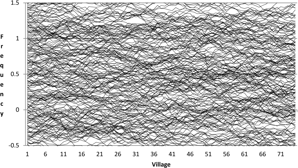
Figure 1.
Recessive allele frequencies at 200 loci in 75 villages prior to truncation.
Figure 1.
Recessive allele frequencies at 200 loci in 75 villages prior to truncation.
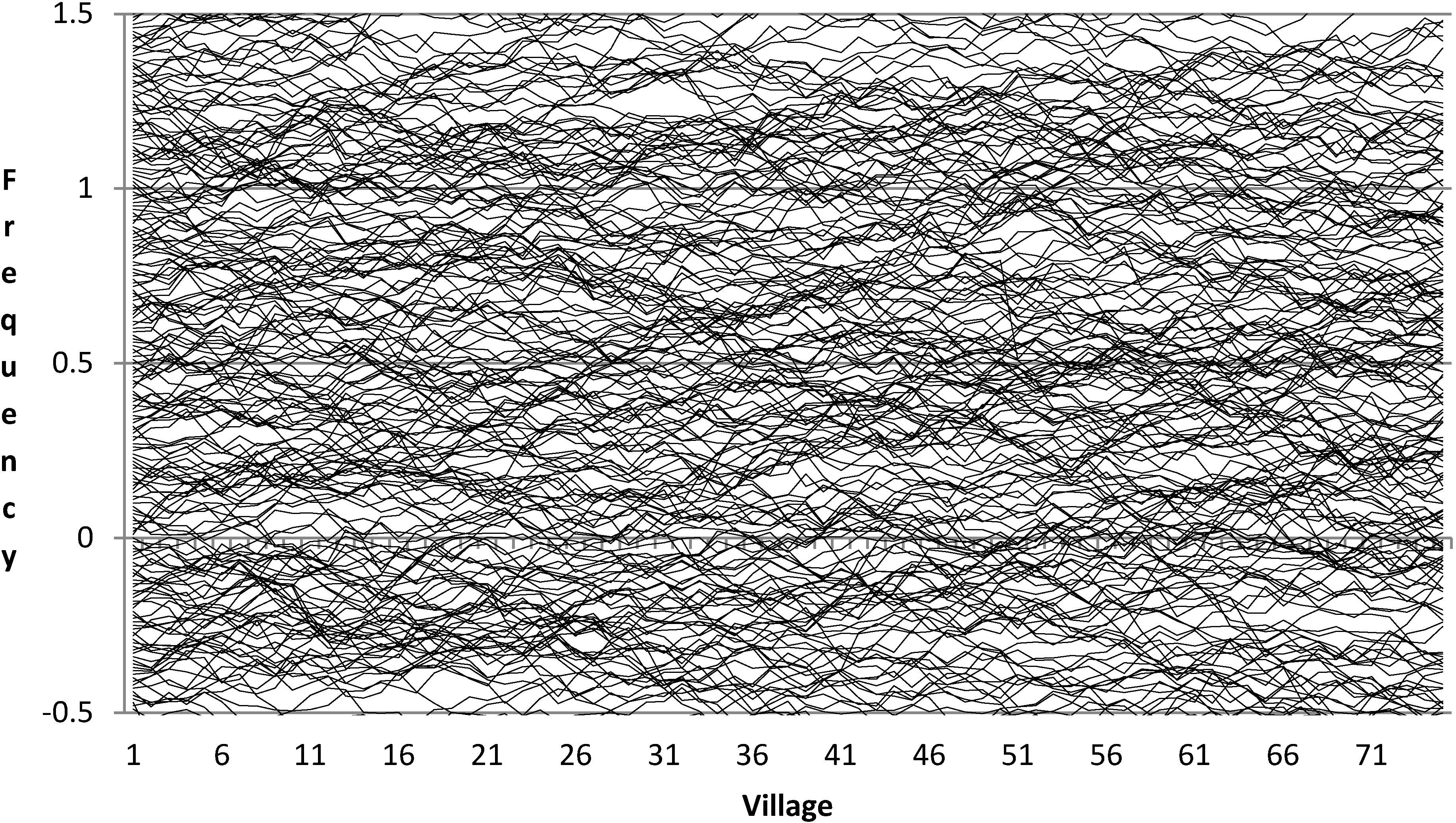
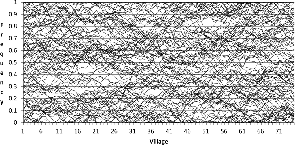
Figure 2.
Recessive allele frequencies at 200 loci in 75 villages after truncation. Only loci with (0 < R < 1) shown.
Figure 2.
Recessive allele frequencies at 200 loci in 75 villages after truncation. Only loci with (0 < R < 1) shown.

Given the above procedures, the typical community will have about 100 polymorphic loci, with recessive (and dominant) frequencies distributed more or less uniformly between 0 and 1 (by ‘polymorphic’ I mean here that both dominant and recessive alleles occur at the locus). This number of loci was not chosen arbitrarily, but was arrived at through a trial and error process so as to comport with findings from IQ family and consanguinity studies. The methods for simulating families and consanguinity are explained in detail in Mingroni [10]. Once the choice was made in the present model to have allele frequencies uniformly distributed between 0 and 1, the necessary value for the D parameter was chosen to be 0.8 to comport with observed IQ family correlations (see [10], Figure 2). It was then determined through trial and error that about 100 polymorphic genes were necessary to comport with inbreeding depression of about three IQ points in the offspring of first cousins. This is somewhat more than the 68 genes that were necessary to comport with consanguinity studies when the recessive frequency was assumed to be 0.5 at all loci instead of being distributed uniformly between 0 and 1.0 (see [10], Table 4 and Figure 1B).
Having generated allele frequencies at all loci in all communities, the next step is to stochastically generate genotypes for a large number of individuals in each community and calculate each individual’s intelligence level from Equation (1) above. We then have individuals from the first community mate with individuals from increasingly distant communities. The children’s genotypes are generated based on the parents’ genotypes and the laws of Mendelian inheritance, as discussed in Mingroni [10], and their intelligence level is calculated using Equation (1). Table 1 lists the results of mating between individuals from increasingly distant communities. The first row shows the results of mating between the first community and the fifth community and the last row shows the results of mating between the first community and the 75th community.

Table 1.
Results of the simulation of inter-village mating.
| Village | μ Parents | σ Parents | μ Children | σ Children | μc-μp/σp (FE) |
|---|---|---|---|---|---|
| 5 | 109.44 | 3.20 | 109.54 | 3.18 | 0.032 |
| 15 | 109.27 | 3.24 | 109.62 | 3.19 | 0.109 |
| 25 | 109.11 | 3.29 | 109.70 | 3.20 | 0.181 |
| 35 | 109.29 | 3.30 | 110.13 | 3.20 | 0.254 |
| 45 | 109.21 | 3.33 | 110.28 | 3.21 | 0.322 |
| 55 | 109.15 | 3.35 | 110.44 | 3.21 | 0.387 |
| 65 | 109.07 | 3.37 | 110.57 | 3.21 | 0.450 |
| 75 | 109.04 | 3.41 | 110.77 | 3.22 | 0.509 |
The typical rate of gain on common test batteries has been about three points per decade, or about 0.5 standard deviations per generation. An intergenerational gain of this magnitude occurs when the parents are about 75 communities apart. This would suggest that couples in which the partners come from opposite ends of the Parma valley might reasonably expect to have children who manifest an intergenerational IQ gain in line with observed values. As a point of reference, the total population of the 74 parishes studied represented only about 0.5% of the total population of Italy in 1960. Presumably, going outside your valley could cause even larger intergenerational gains. Of course, gains on certain tests, such as Raven’s matrices have increased much faster, about seven points per decade in some cases. However, the present model was constrained primarily by the need to comport with only a three point IQ deficit in the offspring of first cousins; and this figure came from a study that used a Wechsler battery [78]. As mentioned above, our best estimate of inbreeding for the Raven’s is about eight points in the offspring of first cousins [96] (see also [97]). A model designed to comport with this larger inbreeding effect would also predict proportionately larger Flynn effects on Raven’s.
There are some features of the present model worth pointing out. First, in addition to the 100 polymorphic loci (i.e., loci that have both dominant and recessive alleles), there are also about 50 loci in each community at which the dominant allele is fixed; these are not shown in Figure 2. They result mainly from those loci at which the recessive frequency was initially set at a negative value and then truncated to zero. These loci add 50 to the mean intelligence level of each village, but contribute nothing to the variance of intelligence within each community. Importantly, though, it is not the same 50 loci in each community; a particular dominant allele might be fixed in some communities, but only very common in others. These loci do not affect the results as they relate to intelligence, which is measured on an ordinal scale (or at best an interval scale); but by influencing the mean, they decrease the coefficient of variation, which must comport with observed findings of traits that are measured on a ratio scale, such as height.
Although the choice that led to this number of loci with fixed dominants was somewhat arbitrary, the resulting coefficient of variation has turned out quite close to that observed in adult height (~3%). In addition, the relative effect of inbreeding on height is about the same as for IQ [78]. Therefore, the present model could just as easily explain the secular trend in height with only slight modifications. One would first have to replace “intelligence” in Equation (1) with “height,” and instead of adding +1 and +D dimensionless units for the different genotypes, one would have to add about +1.5 cm and +1.2 cm, respectively. Explaining the trends in other traits and conditions would follow the same pattern, except that in the case of threshold conditions one would have to replace the dependent variable in Equation (1) with something like “genetic liability to asthma.”.
Perhaps the most salient feature of the present model is that there are potentially an almost infinite number of genotypes that can all lead to the same phenotype. For example, we have posited about 200 loci. The average individual has an IQ-increasing genotype (double dominant or heterozgyous) at only about 100 of them; but the 100 IQ-increasing loci could be a very different subset of all the loci in different communities. In theory at least, one community could have IQ-increasing genes at loci 1 to loci 100, while another community could have IQ-increasing genes at loci 101 to 200. If individuals from these communities were to mate, the intergenerational gains would be enormous. The overall number of IQ-increasing genes in any given population will likely be bounded by selective pressures at some stable level. However, the exact genetic pathway by which individual communities achieve such optimal brain physiology in the model can vary slightly from one town to the next, and eventually become quite large as you get far enough away.
It goes without saying that the present model must represent a grossly oversimplified version of what might be occurring at the genetic level. Some obvious future steps for this approach would be to include such things as assortive mating, environmental influences, and selective pressures. Future efforts could also posit variability across the population in the effects of heterosis, which would induce predicted positive correlations among all the traits and conditions that display directional dominance, and which could then be compared to observed intercorrelations among traits, such as that between height and IQ. Future models will also have to comport with observed secular increases in heterozygosity. Although the present model could certainly be improved, it is unlikely that future refinements will change the basic result presented here, namely, that large secular gains as a result of heterosis are possible given existing genetic data and a reasonable set of assumptions. In fact, if anything, future investigations are apt to identify scenarios in which less genetic change can account for more secular change. In an earlier work, Mingroni [12] pointed out that the impact of heterosis tends to be relatively larger when the recessive alleles are rare, whereas, in the present model, they are distributed more or less uniformly between 0 and 1, so there is likely room for improvement in this respect.
More than anything else, the above exercise demonstrates that quantifying the potential effect of heterosis on secular trends cannot be eyeballed (e.g., [125], pp. 101–102). At a minimum, it requires detailed population genetic data; and even with such data, exhausting all the possibilities cannot be done on the back of an envelope. Even in cases such as the present IQ model, or a similar height model, where the modeling process is greatly constrained by the results of consanguinity studies, a plausible scenario can be imagined whereby a substantial heterosis effect is expected. In the case of traits and conditions where we lack such consanguinity studies, the potential effect of heterosis is currently completely unconstrained. At present, therefore, any secular change in heterozygosity could be responsible for indefinitely large changes in the incidence of conditions such as asthma, myopia and autism, as the genes for these conditions could have practically any structure. Given the serious nature of several of the traits and conditions that have undergone change, we have an obligation to leave no stone unturned in searching for their cause. The above exercise indicates that heterosis may be the largest unturned stone in view.
8. Conclusions
A perennial source of tension in science is that between holism and reductionism. While it is true that one sometimes cannot see the forest for the trees, it is equally true that a forest is a complex ecosystem that cannot be fully appreciated by the view from an orbital satellite alone; a microscope is also required. Like a forest, human cognition is complicated. Understanding the nature and cause of the secular changes in IQ will likely require the ability and willingness to zoom in and out as necessary and view the situation from different perspectives. The suggestions put forward above are generally quite narrow in their scope when viewed separately. How do children compare to parents? How do siblings compare? Has brain physiology changed? How do we boost the traits and have confidence that our interventions have had an effect? What is the potential contribution of genetic changes? What is the subtest profile of the changes.
While we still have many narrow reductionist questions to answer, interpreting the results will surely benefit from a broader perspective. To take just one example, consider the evidence of increasing incidence of autism. Most autism researchers are totally unaware that IQ scores have been rising, and most Flynn effect researchers are only vaguely aware from news reports that autism rates appear to be rising. It is quite possible, though, that the two trends are related. It is not difficult to imagine physiological brain changes that lead to generally improved test performance, but that also have negative consequences when they go too far (e.g., [126]). Taking this possibility seriously has immediate implications for the study of both trends.
Consider first the perspective of the autism researcher. Some studies have found that the rise in autism diagnoses has been accompanied by a decline in children diagnosed as mentally retarded (MR), based on their low IQ [38]. One interpretation of this result is that a percentage of children with the autistic phenotype, who would have previously been diagnosed as MR, are now more likely to receive an autism diagnosis. However, knowing that IQ scores have been rising suggests an alternative explanation. Rather than shifting children from MR to autism through changing diagnostic criteria, it may be that the decline in MR is due to generally rising IQ, which in turn is due to brain changes that also increase the risk of autism. From the perspective of the IQ researcher, evidence of no IQ gains among the highest scorers would suggest causal factors that mainly affect low scorers. Without knowledge of the autism trend, no thought would be given to the possibility that there are effects at the upper end of the IQ distribution, not in the form of higher IQ, but in the form of increased autism. I should emphasize that this is only an example; there is actually some good evidence for diagnostic changes from MR to autism, and not all IQ studies report smaller gains among high scorers. The point is simply that a broader perspective on things can potentially be helpful.
Dawkins once quipped that “reductionism is a dirty word, and a kind of ‘holistier than thou’ self-righteousness has become fashionable” [127]. Of course, those who actually do science know that viewing things holistically is not as simple as putting on a new pair of spectacles. There are millions of empirical findings out there, most of which have nothing to do with the problem at hand. Stumbling across the truly relevant facts takes time, effort, and more than a little luck. At the risk of sounding self-righteous, though, I would suggest that solving the mystery that is the Flynn effect really is going to require a more holistic view; analyses of IQ test data alone probably will not be enough. It might be brain MRI studies that hold the key. It might be genetic data. Intervention studies to boost IQ might break the current logjam. Sibling studies look promising. It may be all of the above, or none of them. In the meantime, all any of us can do is keep plodding along, with our heads up and eyes open to possibility that the answer may come from unexpected quarters, outside our own specific domain of expertise.
Conflicts of Interest
The author declares no conflict of interest.
References
- Flynn, J.R. The mean IQ of Americans: Massive gains 1932 to 1978. Psychol. Bull. 1984, 95, 29–51. [Google Scholar] [CrossRef]
- Flynn, J.R. Massive IQ gains in 14 nations: What IQ tests really measure. Psychol. Bull. 1987, 101, 171–191. [Google Scholar] [CrossRef]
- Williams, R.L. Overview of the Flynn effect. Intelligence 2013, 41, 753–764. [Google Scholar] [CrossRef]
- Gottfredson, L.S. Why g matters. Intelligence 1997, 24, 13–23. [Google Scholar] [CrossRef]
- Hunt, E. What makes nations intelligent? Perspect. Psychol. Sci. 2012, 7, 284–306. [Google Scholar]
- Floud, R.; Fogel, R.W.; Harris, B.; Hong, S.C. The Changing Body: Health, Nutrition, and Human Development in the Western World since 1700; Cambridge University Press: Cambridge, UK, 2011. [Google Scholar]
- Lynn, R.; Vanhanen, T. IQ and Global Inequality; Washington Summit Publishers: Augusta, GA, USA, 2006. [Google Scholar]
- Lynn, R.; Cheng, H. Differences in intelligence across thirty-one regions of China and their economic and demographic correlates. Intelligence 2013, 41, 553–559. [Google Scholar] [CrossRef]
- Murray, C. IQ and economic success. Public Interest 2007, 128, 21–35. [Google Scholar]
- Mingroni, M.A. Resolving the IQ paradox: Heterosis as a cause of the Flynn effect and other trends. Psychol. Rev. 2007, 114, 806–829. [Google Scholar] [CrossRef] [PubMed]
- Woodley, M.A. The social and scientific temporal correlates of genotypic intelligence and the Flynn effect. Intelligence 2012, 40, 189–204. [Google Scholar] [CrossRef]
- Mingroni, M.A. The secular rise in IQ: Giving heterosis a closer look. Intelligence 2004, 32, 65–83. [Google Scholar] [CrossRef]
- Woodley, M.A. Heterosis doesn’t cause the Flynn effect: A critical examination of Mingroni (2007). Psychol. Rev. 2011, 118, 689–693. [Google Scholar] [CrossRef] [PubMed]
- Bock, R.D.; Sykes, R.C. Evidence for continuing secular increase in height within families in the United States. Am. J. Hum. Biol. 1989, 1, 143–148. [Google Scholar] [CrossRef]
- Plomin, R.; DeFries, J.C. Genetics and intelligence: Recent data. Intelligence 1980, 4, 15–24. [Google Scholar] [CrossRef]
- Vinkhuyzen, A.A.E.; van der Sluis, S.; Maes, H.H.M.; Posthuma, D. Reconsidering the heritability of intelligence: Taking assortative mating and cultural transmission into account. Behav. Genet. 2012, 42, 187–198. [Google Scholar] [CrossRef] [PubMed]
- Sundet, J.M.; Eriksen, W.; Borren, I.; Tambs, K. The Flynn effect in sibships: Investigating the role of age differences between siblings. Intelligence 2010, 38, 38–44. [Google Scholar] [CrossRef]
- Black, S.E.; Devereux, P.J.; Salvanes, K.G. Like Father, Like Son? A Note on the Intergenerational Transmission of IQ Scores; IZA Discussion Paper #2651; Institute for the Study of Labor (IZA): Bonn, Germany, 2008. [Google Scholar]
- Myrskyla, M.; Silventoinen, K.; Jelenkovic, A.; Tynelius, P.; Rasmussen, F. Is later better or worse? Association of advanced parental age with offspring cognitive ability among half a million young Swedish men. Am. J. Epidemiol. 2013, 177, 649–655. [Google Scholar] [CrossRef] [PubMed]
- Woodley, M.A.; Meisenberg, G. In the Netherlands the anti-Flynn effect is a Jensen effect. Pers. Ind. Differ. 2013, 54, 871–876. [Google Scholar] [CrossRef]
- Sundet, J.M.; Barlaug, D.G.; Torjussen, T. The end of the Flynn effect? A study of secular trends in mean intelligence test scores of Norwegian conscripts during half a century. Intelligence 2004, 32, 349–362. [Google Scholar]
- Terraciano, A. Secular trends and personality: Perspectives from longitudinal and cross-cultural studies—Commentary on Trzesniewski and Donnelan. Perspect. Psychol. Sci. 2010, 5, 93–96. [Google Scholar] [CrossRef]
- Trzesniewski, K.H.; Donellan, M.B. Rethinking “Generation Me”; a study of cohort effects from 1976–2006. Perspect. Psychol. Sci. 2010, 5, 58–75. [Google Scholar] [CrossRef]
- Smits, I.A.; Dolan, C.V.; Vorst, H.C. M.; Wicherts, J.M.; Timmerman, M.E. Cohort differences in big five personality factors over a period of 25 years. J. Pers. Soc. Psychol. 2011, 100, 1124–1138. [Google Scholar] [CrossRef] [PubMed]
- Hatton, T.J.; Bray, B.E. Long run trends in the heights of European men, 19th–20th centuries. Econ. Hum. Biol. 2010, 8, 405–413. [Google Scholar] [CrossRef] [PubMed]
- Cho, G.J.; Park, H.T.; Shin, J.H.; Hur, J.Y.; Kim, Y.T.; Kim, S.H.; Lee, K.W.; Kim, T. Age at menarche in a Korean population: Secular trends and influencing factors. Eur. J. Pediatr. 2010, 169, 89–94. [Google Scholar] [CrossRef] [PubMed]
- Morris, D.H.; Jones, M.E.; Shoemaker, M.J.; Ashworth, A.; Swerdlow, A.J. Secular trends in age at menarche in women in the UK born 1908–93: Results from the Breakthrough Generations Study. Paediatr. Perinat. Epidemiol. 2011, 25, 394–400. [Google Scholar] [CrossRef] [PubMed]
- CDC. Increasing prevalence of parent-reported attention deficit/hyperactivity disorder among children—United States, 2003 and 2007. MMWR 2010, 59, 1439–1443. [Google Scholar]
- CDC. Prevalence of autism spectrum disorders—Autism and Developmental Disabilities Monitoring Network, 14 sites, United States, 2008. MMWR 2012, 61, 1–19. [Google Scholar]
- Medland, S.E.; Duffy, D.L.; Wright, M.J.; Geffen, G.M.; Martin, N.G. Handedness in twins: Joint analysis of data from 35 samples. Twin Res. Hum. Genet. 2006, 9, 46–53. [Google Scholar] [CrossRef] [PubMed]
- Shih, Y.F.; Hsiao, C.K.; Chen, C.J.; Chang, C.W.; Hung, P.T.; Lin, L.L.K. An intervention trial on the efficacy of atropine and multi-focal glasses in controlling myopic progression. Acta Ophthalmol. Scand. 2001, 79, 233–236. [Google Scholar] [CrossRef]
- Vitale, S.; Sperduto, R.D.; Ferris, F.L. Increased prevalence of myopia in the United States between 1971–1972 and 1999–2004. Arch. Ophthalmol. 2009, 127, 1632–1639. [Google Scholar] [CrossRef]
- Miller, A.K.H.; Corsellis, J.H. Evidence for a secular increase in brain weight during the last century. Ann. Hum. Biol. 1977, 4, 253–257. [Google Scholar] [CrossRef] [PubMed]
- Greiner, T.M.; Gordon, C.C. An Assessment of long-Term Changes in Anthropometric Dimensions: Secular Trends of U. S. Army Males; Technical Report-Natick/TR-91/006; United States Army Natick Research, Development and Engineering Center: Natick, MA, USA, 1990. [Google Scholar]
- Westcott, D.J.; Jantz, R.L. Assessing craniofacial secular change in American Blacks and Whites using geometric morphometry. In Modern Morphometrics in Physical Anthropology; Slice, D.E., Ed.; Kluwer Academic/Plenum Publishers: New York, NY, USA, 2005; Chapter 10; pp. 231–245. [Google Scholar]
- Lynn, R. The role of nutrition in secular increases of intelligence. Pers. Ind. Differ. 1990, 11, 273–285. [Google Scholar] [CrossRef]
- Lynn, R. What has caused the Flynn effect? Secular increases in the Development Quotients of infants. Intelligence 2009, 37, 16–24. [Google Scholar] [CrossRef]
- Hertz-Picciotto, I.; Delwiche, L. The rise in autism and the role of age at diagnosis. Epidemiology 2009, 20, 84–90. [Google Scholar] [CrossRef] [PubMed]
- Nyhan, B.; Reifler, J.; Richey, S.; Freed, G.L. Effective messages in vaccine promotion: A randomized trial. Pediatrics 2014, 133, e835–e842. [Google Scholar]
- McDaniel, M.A. Big-brained people are smarter: A meta-analysis of the relationship between in vivo brain volume and intelligence. Intelligence 2005, 33, 337–346. [Google Scholar] [CrossRef]
- Storfer, M. Myopia, intelligence, and the expanding human neocortex: Behavioral influences and evolutionary implications. Int. J. Neurosci. 1999, 98, 153–276. [Google Scholar] [CrossRef] [PubMed]
- Hedman, A.M.; van Haren, N.E.M.; Schnack, H.G.; Kahn, R.S.; Hulshoff Pol, H.E. Human brain changes across the lifespan: A review of 56 longitudinal magnetic resonance imaging studies. Hum. Brain Map. 2012, 33, 1987–2002. [Google Scholar] [CrossRef]
- Walhovd, K.B.; Westlye, L.T.; Amlien, I.; Espeseth, T.; Reinvang, I.; Raz, N.; Agartz, I.; Salat, D.H.; Greve, D.N.; Fischl, B.; Dale, A.N.; Fjell, A.M. Consistent neuroanatomical age-related volume differences across multiple samples. Neurobiol. Aging 2013, 32, 916–932. [Google Scholar] [CrossRef]
- Alivisatos, A.P.; Chun, M.; Church, G.M.; Greenspan, R.J.; Roukes, M.L.; Yuste, R. The Brain Activity Map Project and the challenge of functional connectomics. Neuron 2012, 74, 970–974. [Google Scholar] [CrossRef]
- Rodgers, J.L. A critique of the Flynn effect: massive IQ gains, methodological artifacts, or both? Intelligence 1998, 26, 337–356. [Google Scholar]
- Lahey, B.B.; D’Onofrio, B.M. All in the family: Comparing siblings to test causal hypotheses regarding environmental influences on behavior. Curr. Dir. Psychol. Sci. 2010, 19, 319–323. [Google Scholar] [CrossRef] [PubMed]
- Wolf, M.; Musch, J.; Enczmann, J.; Fischer, J. Estimating the prevalence of nonpaternity in Germany. Hum. Nat. 2012, 23, 208–217. [Google Scholar] [PubMed]
- Kimura, M.; Yamazaki, Y.; Mochizuki, M.; Omiya, T. Can I have a second child? Dilemmas of mothers of children with pervasive developmental disorder: A qualitative study. BMC Pregnancy Childbirth 2010, 10, 69. [Google Scholar]
- Jones, W.; Klin, A. Attention to eyes is present but in decline in 2-to-6-month old infants later diagnosed with autism. Nature 2013. [Google Scholar] [CrossRef]
- Kong, A.; Frigge, M.L.; Masson, G.; Besenbacher, S.; Sulem, P.; Magnussen, G.; Gudjonsson, S.A.; Sigurdsson, A.; Jonasdottir, A.; Jonasdottir, A.; et al. Rate of de novo mutations and the importance of father’s age to disease risk. Nature 2012, 488, 471–475. [Google Scholar] [CrossRef] [PubMed]
- Myrskyla, M.; Silventoinen, K.; Jelenkovic, A.; Tynelius, P.; Rasmussen, F. The association between height and birth order: Evidence from 652,518 Swedish men. J. Epidemiol. Community Health 2013, 67, 571–577. [Google Scholar] [CrossRef] [PubMed]
- Jensen, A.R. Uses of sibling data in educational and psychological research. Am. Educ. Res. J. 1980, 17, 153–170. [Google Scholar] [CrossRef]
- Taubman, P. (Ed.) Kinometrics: Determinants of Socioeconomic Success Within and between Families; North-Holland: Amsterdam, The Netherlands, 1977.
- Kenny, D.A.; Kashy, D.A.; Cook, W. Dyadic Data Analysis; Guilford Press: New York, NY, USA, 2006. [Google Scholar]
- Dutton, E.; Lynn, R. A negative Flynn effect in Finland, 1997–2009. Intelligence 2013, 41, 817–820. [Google Scholar] [CrossRef]
- Neisser, U.; Boodoo, G.; Bouchard, T.J., Jr.; Boykin, A.W.; Brody, N.; Ceci, S.J.; Halpern, D.F.; Loehlin, J.C.; Perloff, R.; Sternberg, R.J.; et al. Intelligence: Knowns and unknowns. Am. Psychol. 1996, 51, 77–101. [Google Scholar] [CrossRef]
- Bjerkedal, T.; Kristensen, P.; Skjeret, G.A.; Brevik, J.I. Intelligence test scores and birth order among young Norwegian men (conscripts) analyzed within and between families. Intelligence 2007, 35, 503–514. [Google Scholar] [CrossRef]
- Rodgers, J.L.; Cleveland, H.H.; van den Oord, E.; Rowe, D.C. Resolving the debate over birth order, family size and intelligence. Am. Psychol. 2000, 55, 599–612. [Google Scholar] [CrossRef] [PubMed]
- Ernst, C.; Angst, J. Birth Order: Its Influence on Personality; Springer-Verlag: Berlin, Germany, 1983. [Google Scholar]
- Rodgers, J.L. Are birth order effects on intelligence really Flynn effects? Reinterpreting Belmont and Marolla 40 years later. Intelligence 2013, 42, 128–133. [Google Scholar]
- Fredriks, A.M.; van Buuren, S.; Burgmeijer, R.J.F.; Meulmeester, J.F.; Beuker, R.J.; Brugman, E.; Roede, M.J.; Verloove-Vanhorick, S.P.; Wit, J.-M. Continued positive secular growth change in the Netherlands 1955–1997. Pediatr. Res. 2000, 47, 316–323. [Google Scholar] [CrossRef]
- Van Wierengen, J.C. Secular Growth Changes. In Human Growth: A Comprehensive Treatise; Falkner, F., Tanner, J.M., Eds.; Plenum: New York, NY, USA, 1986; pp. 307–331. [Google Scholar]
- Maddison, A. The World Economy: A Millennial Perspective; OECD: Paris, France, 2001. [Google Scholar]
- Ang, S.C.; Rodgers, J.L.; Wanstrom, L. The Flynn effect within subgroups in the U.S.: Gender, race, income, education, and urbanization differences in the NLSY-children data. Intelligence 2010, 38, 367–384. [Google Scholar] [CrossRef]
- Nisbett, R.E. Intelligence and How to Get It: Why Schools and Cultures Count; Norton: New York, NY, USA, 2009. [Google Scholar]
- Rushton, J.P.; Jensen, A.R. Race and IQ: A theory-based review of the research in Richard Nisbett’s Intelligence and How to Get It. Open Psychol. J. 2010, 3, 9–35. [Google Scholar] [CrossRef]
- Beaton, G.H.; Ghassemi, H. Supplementary feeding programs for young children in developing countries. Am. J. Clin. Nutr. 1982, 35, 864–916. [Google Scholar]
- Clay, E.; Pillai, N.; Benson, C. Food Aid and Food Security in the 1990s: Performance and Effectiveness; Working Paper 113; Overseas Development Institute: London, UK, 1998. [Google Scholar]
- Gorgens, T.; Meng, X.; Vaithianathan, R. Stunting and selection effects of famine: A case study of the Great Chinese Famine. J. Dev. Econ. 2012, 97, 99–111. [Google Scholar] [CrossRef]
- Chen, Y.; Zhou, L.-A. The long-term health and economic consequences of the 1959–1961 famine in China. J. Health Econ. 2007, 26, 659–681. [Google Scholar] [CrossRef]
- Huang, C.; Li, Z.; Wang, M.; Martorell, R. Early life exposure to the 1959–1961 Chinese famine has long-term health consequences. J. Nutr. 2010, 140, 1874–1878. [Google Scholar] [CrossRef]
- Stein, Z.; Susser, M.; Saenger, G.; Marolla, F. Nutrition and mental performance. Science 1972, 178, 708–713. [Google Scholar]
- Beaujean, A.A.; Osterlind, S.J. Using item response theory to assess the Flynn effect in the National Longitudinal Study of Youth 79 children and young adults data. Intelligence 2008, 36, 455–463. [Google Scholar] [CrossRef]
- Ali, A.; Uetake, T.; Ohtsuki, F. Secular changes in relative leg length in post-war Japan. Am. J. Hum. Biol. 2000, 12, 405–416. [Google Scholar]
- Woronkowicz, A.; Cichocka, B.A.; Kowal, M.; Kryst, L.; Sobiecki, J. Physical development of girls from Krakow in the aspect of socioeconomical changes in Poland (1938–2010). Am. J. Hum. Biol. 2012, 24, 626–632. [Google Scholar]
- Schiffman, J.; Pestle, S.; Mednick, S.; Ekstrom, M.; Sorensen, H.; Mednick, S. Childhood laterality and adult schizophrenia spectrum disorders: A prospective investigation. Schizophr. Res. 2005, 72, 151–160. [Google Scholar] [CrossRef] [PubMed]
- Georgiades, S.; Szatmari, P.; Boyle, M. The importance of studying heterogeneity in autism. Neuropsychiatry 2013, 3, 123–125. [Google Scholar] [CrossRef]
- Schull, W.J.; Neel, J.V. The Effects of Inbreeding on Japanese Children; Harper & Row: New York, NY, USA, 1965. [Google Scholar]
- Woodley, M.A. A life history model of the Lynn-Flynn effect. Pers. Ind. Differ. 2012, 53, 152–156. [Google Scholar] [CrossRef]
- Flynn, J.R.; Weiss, L.G. American IQ gains from 1932 to 2002: The WISC subtests and educational progress. Int. J. Test. 2007, 7, 209–224. [Google Scholar] [CrossRef]
- Wicherts, J.M.; Dolan, C.V.; Hessen, D.J.; Oosterveld, P.; van Baal, G.C.M.; Boomsma, D.I.; Span, M.S. Are intelligence tests measurement invariant over time? Investigating the nature of the Flynn effect. Intelligence 2004, 32, 509–537. [Google Scholar] [CrossRef]
- Fox, M.C.; Mitchum, A.L. A knowledge-based theory of rising scores on “culture free” tests. J. Exp. Psychol.: Gen. 2012. [Google Scholar] [CrossRef]
- Shiu, W.; Beaujean, A.A.; Must, O.; te Nijenhuis, J.; Must, A. An item-level examination of the Flynn effect on the National Intelligence Test in Estonia. Intelligence 2013, 41, 770–779. [Google Scholar] [CrossRef]
- Johnson, T.P. Methods and frameworks for crosscultural measurement. Med. Care 2006, 44, S17–S20. [Google Scholar] [CrossRef]
- Spaan, P.E.J.; Dolan, C.V. Cognitive decline in normal ageing and early Alzheimer’s disease: A continuous or discontinuous transition? Behav. Neurol. 2010, 23, 203–206. [Google Scholar]
- Johnson, W.; Bouchard, T.J. Sex differences in mental ability: a proposed means to link them to brain structure and function. Intelligence 2007, 35, 197–209. [Google Scholar]
- Murray, A.L.; Booth, T.; McKenzie, K.; Kuenssberg, R.; O’Donnell, M. Are autistic traits measured equivalently in individuals with and without an autism spectrum disorder? An invariance analysis of the Autism Spectrum Quotient Short Form. J. Autism Dev. Disord. 2014, 44, 55–64. [Google Scholar] [CrossRef] [PubMed]
- Toga, A.W.; Thompson, P.M. Mapping brain asymmetry. Nat. Rev. Neurosci. 2003, 4, 37–48. [Google Scholar] [CrossRef] [PubMed]
- Johnson, W.; Bouchard, T.J., Jr. Sex differences in mental abilities: g masks the dimensions on which they lie. Intelligence 2007, 35, 23–39. [Google Scholar] [CrossRef]
- Boorsboom, D. When does measurement invariance matter? Med. Care 2006, 44, S176–S181. [Google Scholar] [CrossRef]
- Greenfield, P.M. The cultural evolution of IQ. In The Rising Curve: Long-Term Gains in IQ and Related Measures; Neisser, U., Ed.; American Psychological Association: Washington, DC, USA, 1998; pp. 81–123. [Google Scholar]
- Williams, W.M. Are we raising smarter children today? School- and home-related influences on IQ. In The Rising Curve: Long-Term Gains in IQ and Related Measures; Neisser, U., Ed.; American Psychological Association: Washington, DC, USA, 1998; pp. 125–154. [Google Scholar]
- Afzal, M. Consequences of consanguinity on cognitive behavior. Behav. Genet. 1988, 18, 583–594. [Google Scholar] [CrossRef] [PubMed]
- Badaruddoza; Afzal, M. Inbreeding depression and intelligence quotient among North Indian Children. Behav. Genet. 1993, 23, 343–347. [Google Scholar] [CrossRef] [PubMed]
- Bashi, J. Effects of inbreeding on cognitive performance. Nature 1977, 266, 440–442. [Google Scholar] [CrossRef] [PubMed]
- Agrawal, N.; Sinha, S.N.; Jensen, A.R. Effects of inbreeding on Raven matrices. Behav. Genet. 1984, 14, 579–585. [Google Scholar] [CrossRef] [PubMed]
- Nagoshi, C.T.; Johnson, R.C. The ubiquity of g. Pers. Indiv. Differ. 1986, 7, 201–208. [Google Scholar] [CrossRef]
- Jensen, A.R. Effects of inbreeding on mental-ability factors. Pers. Ind. Differ. 1983, 4, 71–87. [Google Scholar] [CrossRef]
- Te Nijenhuis, J.; van der Flier, H. Is the Flynn effect on g?: A meta-analysis. Intelligence 2013, in press. [Google Scholar]
- Jensen, A.R. The g factor: The science of mental ability; Praeger: Westport, CT, USA, 1998. [Google Scholar]
- Nagoshi, C.T.; Johnson, R.C.; DeFries, J.C.; Wilson, J.R.; Vandenberg, S.G. Group differences and first principle-component loadings in the Hawaii Family Study of Cognition: A test of ‘Spearman’s hypothesis.’. Pers. Ind. Differ. 1984, 5, 751–753. [Google Scholar] [CrossRef]
- Dickens, W.T.; Flynn, J.R. Heritability estimates versus large environmental effects: The IQ paradox resolved. Psychol. Rev. 2001, 108, 346–369. [Google Scholar] [CrossRef]
- Carroll, J.B. Human Cognitive Abilities: A Survey of Factor-Analytic Studies; Cambridge University Press: Cambridge, UK, 1993. [Google Scholar]
- Herrnstein, R.J.; Murray, C. The Bell Curve: Intelligence and Class Structure in American Life; Free Press: New York, NY, USA, 1994. [Google Scholar]
- Loehlin, J.C. The strange case of c2 = 0: What does it imply for views of human development? Res. Hum. Dev. 2007, 4, 151–162. [Google Scholar] [CrossRef]
- Heath, S.C.; Gut, I.G.; Brennan, P.; McKay, J.D.; Bencko, V.; Eleonora, F.; Foretova, L.; Georges, M.; Janout, V.; Kabesch, M.; et al. Investigation of the fine structure of European populations with application to disease association studies. Eur. J. Hum. Genet. 2008, 16, 1413–1429. [Google Scholar] [CrossRef] [PubMed]
- Price, A.L.; Helgason, A.; Palsson, S.; Stefansson, H.; St. Clair, D.; Andreassen, O.A.; Reich, D.; Kong, A.; Stefansson, K. The impact of divergence time on the nature of population structure: An example from Iceland. PLoS Genet. 2009, 5, e1000505. [Google Scholar] [CrossRef]
- Colonna, V.; Nutile, T.; Ferrucci, R.R.; Fardella, G.; Aversano, M.; Barbujani, G.; Ciullo, M. Comparing population structure inferred from genealogical versus genetic information. Eur. J. Hum. Genet. 2009, 17, 1635–1641. [Google Scholar] [CrossRef]
- Sebro, R.; Hoffman, T.J.; Lange, C.; Rogus, J.J.; Risch, N.J. Testing for non-random mating: Evidence for ancestry-related assortative mating in the Framingham Heart Study. Genet. Epidemiol. 2010, 34, 674–679. [Google Scholar] [CrossRef] [PubMed]
- Vitart, V.; Carothers, A.D.; Hayward, C.; Teague, P.; Hastie, N.D.; Campbell, H.; Wright, A.F. Increased level of linkage disequilibrium in rural compared with urban communities: A factor to consider in association-study design. Am. J. Hum. Genet. 2005, 76, 763–772. [Google Scholar] [CrossRef]
- Roy-Gagnon, M.; Moreau, C.; Bherer, C.; St. Onge, P.; Sinnett, D.; Laprise, C.; Vezina, H.; Labuda, D. Genomic and genealogical investigation of the French Canadian founder population structure. Hum. Genet. 2011, 129, 521–531. [Google Scholar] [CrossRef] [PubMed]
- Yamaguchi-Kabata, Y.; Nakazono, K.; Takahashi, A.; Saito, S.; Hosono, N.; Kubo, M.; Nakamura, Y.; Kamatani, N. Japanese population structure, based on SNP geneotypes from 7003 individuals compared to other ethnic groups: Effects on population-based association studies. Am. J. Hum. Genet. 2008, 83, 445–456. [Google Scholar] [CrossRef] [PubMed]
- Jakkula, E.; Rehnstrom, K.; Varilo, T.; Pietilainen, O.P.H.; Paunio, T.; Pederson, N.L.; deFaire, U.; Jarvelin, M.R.; Saharinen, J.; Freimer, N.; et al. The genome-wide patterns of variation expose significant substructure in a founder population. Am. J. Hum. Genet. 2008, 83, 787–794. [Google Scholar] [CrossRef] [PubMed]
- Reich, D.; Thangaraj, K.; Patterson, N.; Price, A.L.; Singh, L. Reconstructing Indian population history. Nature 2009, 461, 489–494. [Google Scholar] [CrossRef]
- Wahlund, S. Zuzammensetzung von populationen in und correlation-serscheiunungen von standpunkt der vererbungslehre aus betrachet. Hereditas 1928, 11, 65–106. [Google Scholar] [CrossRef]
- Helgason, A.; Yngvadottir, B.; Hrafnkelsson, B.; Gulcher, J.; Stefansson, K. An Icelandic example of the impact of population structure on association studies. Nat. Genet. 2005, 37, 90–95. [Google Scholar] [PubMed]
- Nails, M.A.; Simon-Sanchez, J.; Gibbs, J.R.; Paisan-Ruiz, C.; Bras, J.T.; Tanaka, T.; Matarin, M.; Scholz, S.; Weitz, C.; Harris, T.B.; et al. Measures of autozygosity in decline: Globalization, urbanization, and its implications for medical genetics. PLoS Genet. 2009, 5, e1000415. [Google Scholar] [CrossRef]
- Rudan, I.; Carothers, A.D.; Polasek, O.; Hayward, C.; Vitart, V.; Biloglav, Z.; Kolcic, I.; Zgaga, L.; Ivankovic, D.; Vorko-Jovic, A.; et al. Quantifying the increase in average human heterozygosity due to urbanization. Eur. J. Hum. Genet. 2008, 16, 1097–1102. [Google Scholar] [CrossRef] [PubMed]
- Campbell, H.; Rudan, I.; Bittles, A.H.; Wright, A.F. Human population structure, genome autozygosity and human health. Genome Med. 2009, 1, 91. [Google Scholar] [CrossRef] [PubMed]
- Kacser, H.; Burns, J.A. The molecular basis of dominance. Genetics 1981, 97, 639–666. [Google Scholar] [PubMed]
- Darwin, C.R. The Effects of Cross- and Self-fertilisation in the Vegetable Kingdom; John Murry London: London, UK, 1873. [Google Scholar]
- Chen, Z.J. Genomic and epigenetic insights into the molecular bases of heterosis. Nat. Rev. Genet. 2013, 14, 471–482. [Google Scholar] [CrossRef] [PubMed]
- Cavalli-Sforza, L.L.; Moroni, A.; Zei, G. Consanguinity, Inbreeding, and Genetic Drift in Italy; Princeton University Press: Princeton, NJ, USA, 2004. [Google Scholar]
- Neel, J.V. Physician to the Gene Pool: Genetic Lessons and Other Stories; Wiley: New York, NY, USA, 1994. [Google Scholar]
- Flynn, J.R. What is Intelligence? Beyond the Flynn Effect; Cambridge University Press: Cambridge, UK, 2007. [Google Scholar]
- Redcay, E.; Courchesne, E. When is the brain enlarged in autism? A meta-analysis of all brain size reports. Biol. Psychiatry 2005, 58, 1–9. [Google Scholar] [CrossRef] [PubMed]
- Dawkins, R. The Extended Phenotype: The Long Reach of the Gene; Oxford University Press: Oxford, UK, 1989. [Google Scholar]
© 2014 by the authors; licensee MDPI, Basel, Switzerland. This article is an open access article distributed under the terms and conditions of the Creative Commons Attribution license (http://creativecommons.org/licenses/by/4.0/).