1. Introduction
The development of technologies that make it possible to obtain data from environments, observed objects, and processes and process them with sufficient speed and efficiency leads to the widespread implementation of cyber-physical systems (CPSs) [
1]. As a part of the operating of these systems, the received information (data) is synchronized with a corresponding physical or information object. The result of such synchronization is a digital twin (DT) of an object, i.e., a model of a complex system. The DT continues to synchronize with the modeled object and reflect its dynamic characteristics that change over time. Such models can be used to conduct digital experiments, implement alternative external scenarios, and predict the behavior of an object in the future without affecting or changing a real prototype.
The issue of building DTs and the simultaneous development of artificial intelligence technologies have led to the emergence of so-called “pure” data-driven modeling “black boxes”, in which a model is created on the basis of deep learning using big data. While the possibility of obtaining such data has been growing in recent times, the cost of storing and processing data has increased along with a rise in data volumes. In addition, for some complex industrial and technological processes, the acquisition of a large amount of data itself can be accompanied by high expenditure and, sometimes, a lack of measurement possibilities. In these cases, the data can be utilized to verify a model built by classical modeling methods based on the physics of an object, including numerical methods for solving corresponding problems of mathematical physics.
The intention to preserve the advantages and eliminate the disadvantages of both types of methods is reflected in the new classifications of existing modeling paradigms [
2,
3,
4]. Physical laws provide interpretability and extrapolation properties to data-driven models which, in turn, connect theoretical models to real objects. We do not aim at repeating or improving the overviews of different models. However, the description of various modeling classes seems essential. Ref. [
2] reviews the concepts of DT modeling and highlights the value of the DT in the modern world and its application in various sectors of the economy. Among the models combining physics and data-based modeling, [
2] points out four categories formed by the mutual integration of the following modeling approaches: physics-based modeling, data-driven modeling, and big data methods. A similar classification can be found in [
5]. The article [
3] focuses on the CPS application and provides a detailed classification of hybrid models, distinguishing among physics-based machine learning modeling classes of algorithms that differ in the nature of interaction between physics-based and machine learning (ML) approaches to modeling. Firstly, these are the methods that utilize physics theory for the preprocessing of data, which then arrive at an input of a neural network in ML. The second type of model comprises those in which prior knowledge of the physics of an object is reflected in an architecture of a network. Thirdly, one of the most popular hybrid modeling methods is underlined, which consists of using physics equations as an additional regularization term in the loss function of an ML model. Similar classes are described in [
6]. In [
3], models in which activation functions are physically interpretable also act as a separate class. In [
4,
7], in addition to those mentioned above, embedding approaches are pointed out, in which data-driven models are used as components of classical physics-based models to speed up, simplify, or replace a numerical solution.
The authors of one of the most cited recent papers on hybrid modeling of complex systems [
8] mention that, among others, they have been inspired by the work [
9] dedicated to the use of neural networks to solve ordinary and partial differential equations. Let us note that in our work [
10], published in 2005, we talk about solving problems of mathematical physics by using both neural networks and real measurements. From the point of view of modern classification, we can regard this approach as a hybrid model with physics-based regularization.
In this article, we consider our previously developed methods of hybrid modeling and their modifications in the context of the modern classification of paradigms for modeling complex dynamic systems. We present the principles of building physics-based network models naturally capable of further adaptation and refinement using measurement data and other additional data.
We have chosen the problem of modeling a system described by a boundary value problem with an unknown parameter as a specific issue of this paper. Problems involving differential equations with unknown parameters frequently arise in the modeling and control of CPS. These parameters can be regarded as dynamic and changing with time according to an unknown law. When describing complex systems, the parameter can characterize the conditions in which the object exists, or a specific part of this object. Thus, the parameter can influence a type of the differential problem under question. It can be considered a hard problem, an ill-posed problem, a problem with a small parameter at the highest derivative, and, accordingly, a problem with a boundary layer, and other types. Let us note that, when solving a problem with an unknown parameter, we do not set to ourselves the task of identifying this parameter, dubbed data-driven discovery of differential equations. As a result of applying methods described below, we obtain a parametric solution that is universal for various parameter values belonging to a predetermined interval that is used in the construction and training of a neural network solution. The resulting pre-trained model can be further adapted by training on the measured data. Based on these measurements, unknown parameters can also be estimated by any means or adjusted using additional training of the network. A similar problem is solved in [
11], where simulating a lake’s temperature is considered. The authors of [
11] use the loss function with physics-based regularization to pre-train a recurrent neural network model before adapting it by means of measurements of a certain lake. They also suggest using the finite element method data as a training dataset.
It is necessary to make a remark about the accuracy of a solution to the problem. Nowadays, there are two fundamentally different approaches to mathematical modeling. The first one is traditional and involves passing from a simulated object to a model in the form of a differential equation (system of equations) with additional conditions (initial, boundary, etc.). Further, this model is considered the object itself and an approximate solution is constructed based on it. The higher the accuracy of such a solution, the more accurate the model of the original real object appears to be. The second approach, which we adhere to, is that the differential model built on the basis of physical principles is certainly approximate. For real complex technical objects, the accuracy of similar models is often low. Therefore, the solution of differential equation(s) with high accuracy has no practical sense. More promising is the construction of an adaptive model that corresponds to the differential equation and additional conditions with reasonable accuracy and the subsequent adaptation of this model to the data of object observations. This approach is especially relevant in a situation when the properties of an object can change during its operation.
The paper [
12] considers hybrid systems, which are a class of problems that cyclically switch between two phases: the first is described by a stiff system of differential algebraic equations of motion (interaction with the ground), the second corresponds to the flight phase and is specified by a non-stiff system. Using a specific problem (hopping single-legged robots) as an example, the authors of [
12] compare various ODE (ordinary differential equation) solvers, including those common in the Matlab package. It is noted that although different solvers work well for different types of problems, due to the constant restart of the numerical solver, the accuracy of the solution diminishes and the cost of computation increases. This problem could be solved with a simple universal approach. Ref. [
13] considers the need to solve a parameterized problem that also arises when studying a wide range of complex physical phenomena, when, while modeling many different possible implementations of the system, large requirements for computational resources lead to the forced use of the apparatus for reducing parametric models. The authors underline the importance of such parametric models in global problems of design, control, optimization, and quantification of uncertainty. The development of a controller that works effectively for all values of model parameters is regarded as an urgent task. Ref. [
14] proposes a solution to a parameterized differential problem by the FEM for an interval parameter based on interval arithmetic. However, as a result they obtain only the corresponding interval boundaries of the solution. Earlier, the authors of the given article studied the construction of a unified solution to one parameterized differential problem, which, for some values of the parameter, is stiff [
15]. The unified neural network approach was applied using various additional information of heterogeneous types to improve the quality of an approximate solution. In [
16], we successfully applied this approach to solve various types of problems with parameters. A stiff differential problem and a differential algebraic problem with different numbers of solutions were solved. In the catalyst problem, we solved the problem in a region that is wider than the domain of existence of the solution to the differential equation. The authors of [
17] also used trainable neural networks with a single hidden layer to obtain a differentiable closed-form solution for a class of parameterized initial-value systems with varying degrees of stiffness. Ref. [
18] highlights the growing interest in the development of numerical methods for solving similar problems and suggests a method based on a rational spectral collocation. Adaptive grid methods are considered in [
19,
20,
21,
22]. Ref. [
23] proposes a special neural network for solving linear singularly perturbed differential equations with initial and boundary values. We note the advantage of low computational costs of the application of neural network models after the training phase. However, when describing systems with uncertainty, the structure of the differential problem itself may often be unknown in advance. Thus, the need arises for building an analytical solution that does not require real-time training and reflects the model under consideration for different parameter values. This approach related to physics-based network architectures is presented in this paper as an extension of the multilayered techniques [
24].
We have planned the structure of this manuscript as follows.
Section 2 discusses the methods of constructing the models of systems described in the form of a classical non-parameterized boundary value problem. Through expansion in basis functions, the basic principles of the finite element method (FEM) [
25] as one of the “pure” physics-based modeling methods, and the general neural network approach [
10] as a variant of ML modeling with physics-based regularization, are presented. In
Section 2.3, the ML model is proposed to be improved by using prior knowledge of the physics of an object in the form of a training data set. The values of an FEM solution in the nodes are utilized instead of measurement results for additional training of the neural network model. A less popular modeling class, named physics-based network architectures, is suggested in
Section 2.4 as a special multilayered model based on classical numerical methods.
Section 3 is devoted to methods of constructing models in cases where the parameters included in the corresponding equations may not be known. In particular, guidance for using the methods described in
Section 2.3 and
Section 2.4 for parameterized problem setting is discussed. We want to emphasize that this certain problem statement is our major interest in this work. Approaches to solving the problem with a fixed parameter are presented to facilitate an understanding of methods for solving parameterized problems.
Section 4 features the parameterized singular perturbation problem and presents the results of applying the previously described methods to the model construction.
Section 5 contains conclusions and considerations for future research.
2. Materials and Methods. Ordinary Problems
To clarify the methods, let us formulate as an example a boundary value problem
where
A is a differential operator, i.e., an algebraic expression containing derivatives of an unknown function
u,
B is some operator specifying the boundary conditions, and
is the boundary of some domain.
We seek an approximate solution in the form of an expansion in basis functions
Searching for a solution in form (
2) is usually called the Galerkin method. Its special cases include different variants of the FEM and neural network models, in which equations based on physics are used as an additional term for the regularization of the loss function. In this case, this models differ in the features of the selection of basis functions and parameters
.
2.1. Methods with Fixed Basis Functions
First, let us distinguish a group of methods in which basis functions
are fixed and only parameters
are adjusted. The extreme learning machine (ELM) algorithm [
26] for single hidden layer feedforward neural networks (SFLNs) randomly chooses internal weights and biases of basis functions and then analytically obtains the output weights
. Ref. [
27] proposes the incremental method for SFLNs and also shows its efficiency for SLFNs with piecewise continuous basis functions.
A similar approach is typical for the simplest version of the FEM. There are two conventional approaches to finding the parameters
. The first, the most common of them, is that the space with the dot product
is regarded as the space in which the solution is sought. The simplest version of such a dot product is the product in the integral form
. In this way, the parameters
are found from the condition of orthogonality of the residual of Equation (
1) to all the basis functions
It is easy to ascertain that they can be found as a solution to the system
If the integral cannot be calculated explicitly, it can be calculated by using cubature formulas or through the mean value
Basis functions usually satisfy the homogeneous boundary condition
. To satisfy the inhomogeneous boundary condition, additional term
is added to sum (
2). This term satisfies the inhomogeneous boundary condition
. The sum takes the form
.
Accordingly, the substitution
into (
3) yields a linear system of the form
Or, for the discrete form of the loss function,
This approach is referred to as the collocation method.
The above basis functions are usually chosen so that their supports intersect only for a small number of functions, while the matrix of system (
4) is sparse, which greatly speeds up the solution procedure.
The second approach is that the quality of the solution to problem (
1) is characterized by a loss function (dubbed the error functional or error function)
J, the minimization of which leads to the needed parameters
.
As shown above, we can use the integral form of the loss function, for example, .
If it is difficult to calculate the dot product explicitly, then we can use the discrete form
The finite element method is characterized by using basis functions (elements) with a compact support localized in small subdomains of . In this case, the supports of the basis functions intersect and cover the entire domain . With this method, if the supports of the basis functions intersect only with a small number of supports of other basis functions, the matrix of the system turns out to be sparse.
For piece-wise linear elements, direct application of Formula (
4) may be impossible due to the absence of derivatives of the required order. In several cases, this problem can be solved by applying the Stokes formula or by the corresponding version of the integration by parts formula.
2.2. Physics-Based Neural Network Approach
When solving stiff problems, the previously considered approach with fixed basis functions does not work well, and these functions have to be adjusted during the solving process. In [
28], the ELM learning algorithm with a tunable basis function is studied.
At first glance, the general neural network approach is similar to the previous ones, only expansion (
2) is specified by the expression
By solving the optimization problem for a certain loss function, both linear parameters and vector parameters (weights and biases) are adjusted. Functions typical of neural networks are used as basis functions. These are usually radial basis functions (RBFs) or perceptron-type functions with sigmoid basis functions.
2.2.1. Multilayer Perceptron
This type of neural network is the most widely used and researched. Let us describe its structure. Let the input be an m-dimensional vector. Linear combinations of coordinates of the input of the form are fed to the input of the first layer of neurons. The coefficients of these combinations are named the weights of the first layer. Each neuron acts as a one-dimensional non-linear function dubbed an activation function. Linear combinations of outputs of neurons are fed to the next layer, and linear combinations of outputs of neurons of the last layer form the output of the network. An additional neuron, whose output always equals 1, is often added to all or some of the layers. Its meaning is the same as adding bias to linear regression, i.e., in fact, the subtraction of a constant value. Experience has shown that this greatly improves network training. In addition, an input is often added, whose value always equals 1. Usually, an activation (basis) function is a function that approximates in form to . Its meaning is to split the space into two half-spaces by hyperplanes and as long as a bias is used. In one of the half-spaces, the output of the neuron is equal to +1; in the other it is equal to −1. If we take not only one neuron, but a layer of neurons, the entire space is divided by hyperplanes into subsets, each of which corresponds to its own set of outputs of neurons of this layer. In this way, the network output is obtained as a piecewise constant function. Usually, instead of function , smooth functions are used, which makes it possible to calculate the derivatives and apply gradient methods to train the network. In this case, it is advisable that the calculation of the derivatives of the activation function requires a minimum of additional operations. For such functions, the network does not produce a piecewise constant, but a smoothed dependence. Here are some examples.
The activation function recommended in the works of A.N. Gorban and his students has the form and . One function is more commonly used, namely . Here, . An asymmetric version of this function is sometimes used , where . Other functions are also applied, for example, , .
Let us describe the functioning of the multilayer perceptron more formally. Denote the vector of inputs of the l-th layer , and the vector of outputs . Then the network is described by recurrence relations , . Here is a network input and is a network output. is a matrix of weights of the l-th layer, and is the activation function, which acts coordinate-wise.
Application of gradient methods of network training, i.e., minimizing the error, requires calculating the derivatives of the network output with respect to the weights, which are easy to obtain using the formula for differentiating a complex function.
To determine the desired derivatives, calculations are performed using the formula
Matrices
are calculated by counting the network outputs. In accordance with (
10), computations begin at the last layer and move to the first. In the literature on neural networks, the calculation of derivatives by this algorithm is often combined with calculations by the gradient descent method, and this hybrid is called the back-propagation method. This algorithm is generalized in the form of automatic differentiation and is widely used in training neural networks, including in [
8].
2.2.2. Radial Basis Function Networks
The main difference between this type of network and the perceptron is that each neuron is responsible for local approximation in the vicinity of some point, and not for the difference between the values of the function in half-spaces, as in the case of the perceptron. Hence the conclusion that the perceptron is best used to simulate problems with jumps, such as phase transitions and shock waves. RBF networks are preferred for applications where a sufficiently smooth solution is to be expected.
In this case, the activation function has the form . Here, is the center weight, is a scale parameter for each neuron of a hidden layer, and is some metric on . Parameters , , and are selected during network. Two fundamentally different approaches can be applied to the adjustment of centers.
We consider fixed centers in the distribution domain of the input. They can be chosen regularly in this area according to certain principles or randomly due to some probabilistic law. Each acts the same as parameters and included in the process of loss function optimization.
There are also two options for choosing parameters . First, , where is a certain size of the considered domain. This method is utilized, as a rule, if the centers are selected in a regular way. Alternatively, is defined by some method of non-linear optimization in conjunction with other parameters. We can apply an intermediate option assuming that and adjusting as one of the optimized parameters. There are a few options left for . If they are found separately, then a linear system is obtained. If we mutually select all the coefficients, then we can use some non-linear optimization algorithm.
To solve problem (
1) it is natural to choose the loss function in the form
, where
corresponds to obeying the equation and
to obeying the boundary condition. Usually, due to the impossibility of calculating integrals explicitly, a discrete form is used. Thus,
and
Our experience of applying neural networks [
29] allows making some remarks about the choice of points
and
. They can be chosen inside
(or in a wider set
if it is necessary to ensure sufficient smoothness of an approximate solution up to the boundary) and on the boundary in a regular way; for example, uniformly in the case of a bounded domain or according to the normal probability law if it is unbounded.
It is often more appropriate to utilize a set of points selected according to the probabilistic distribution law and re-generated after a certain number of learning epochs (optimization steps) using a constant (or other) probability density. This ensures more stable learning.
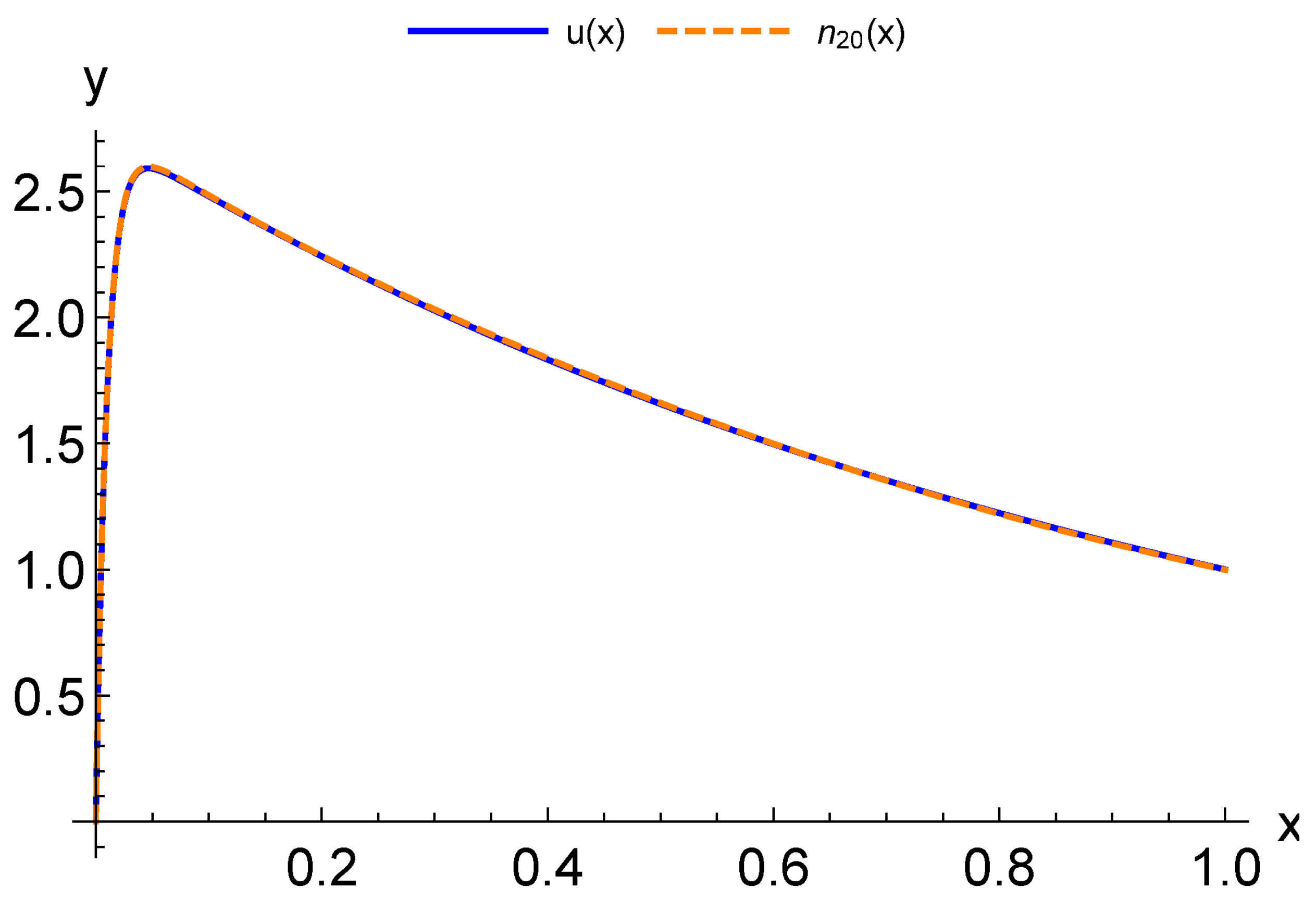
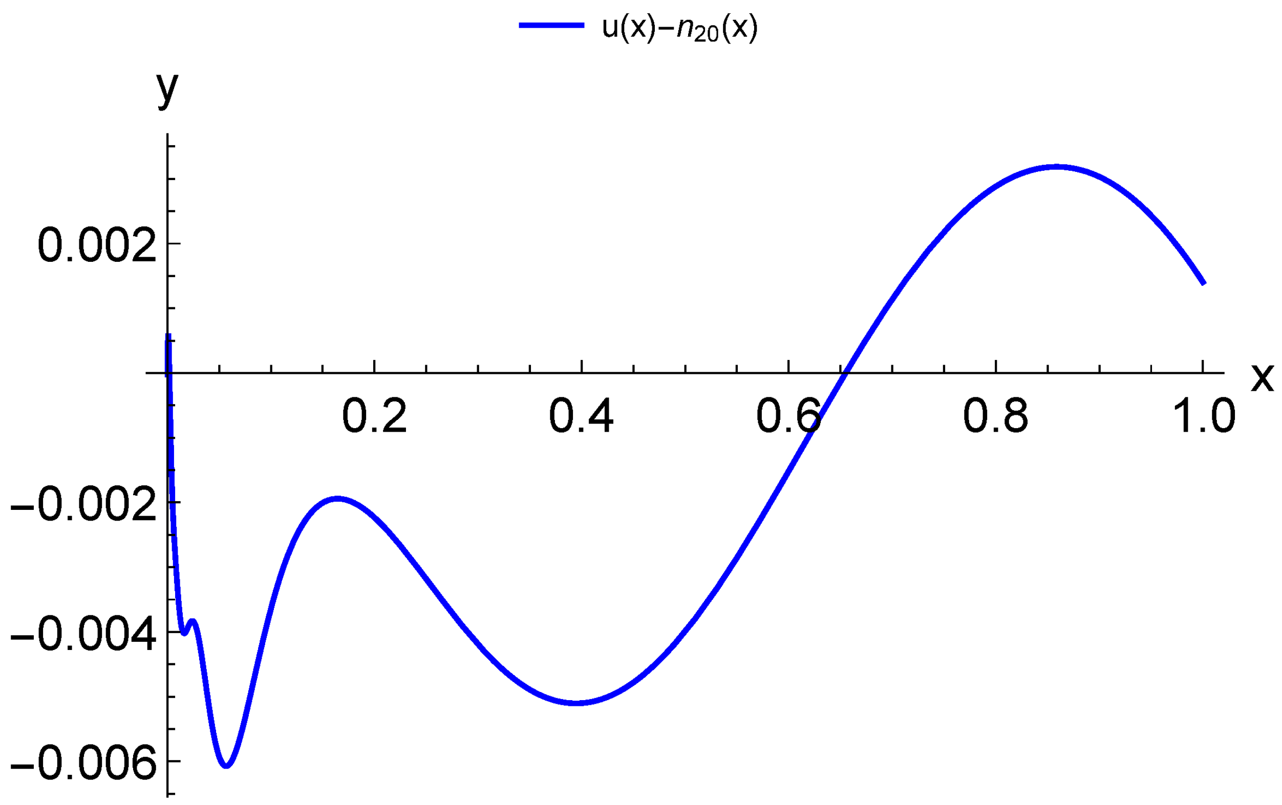
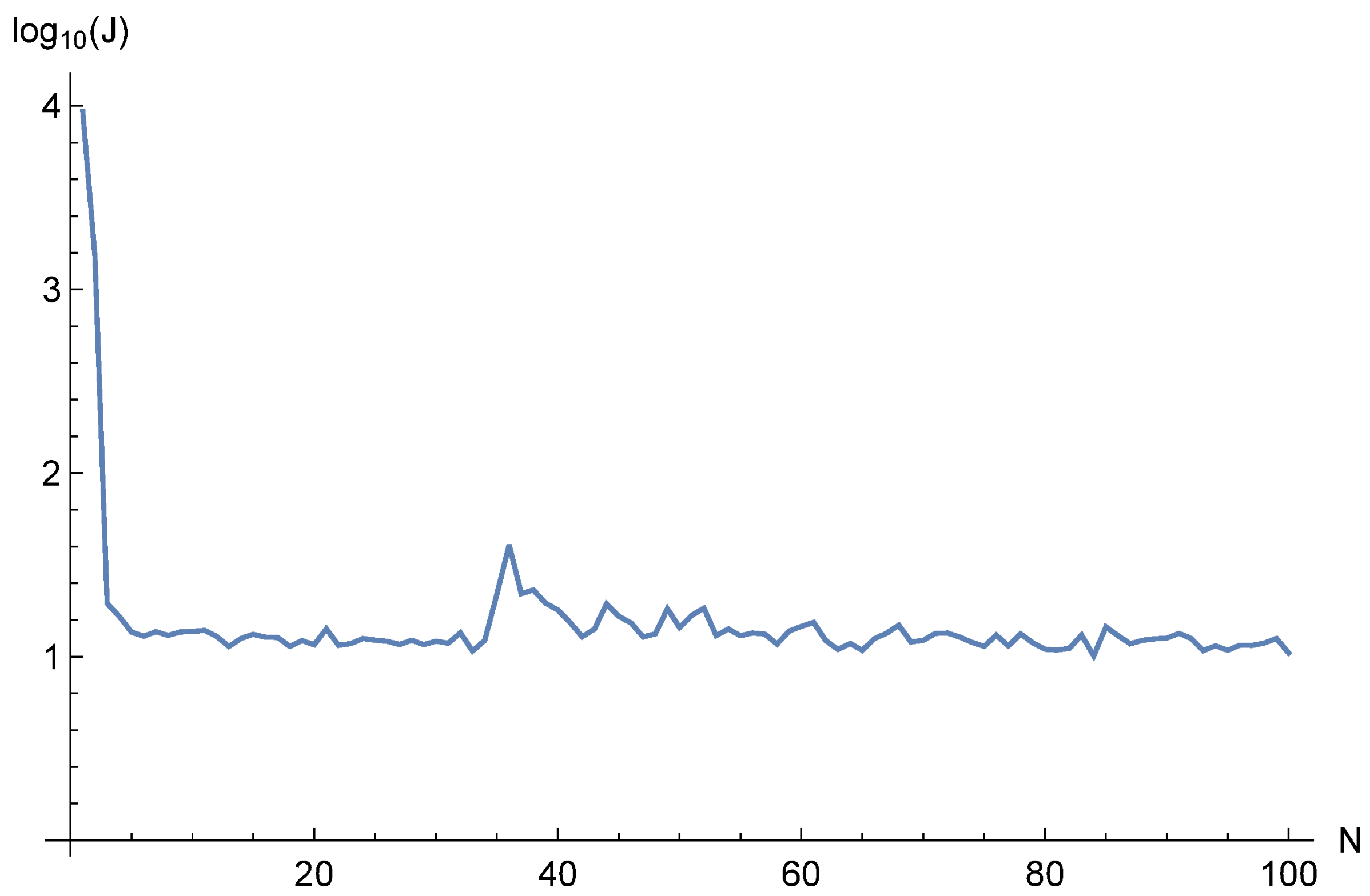
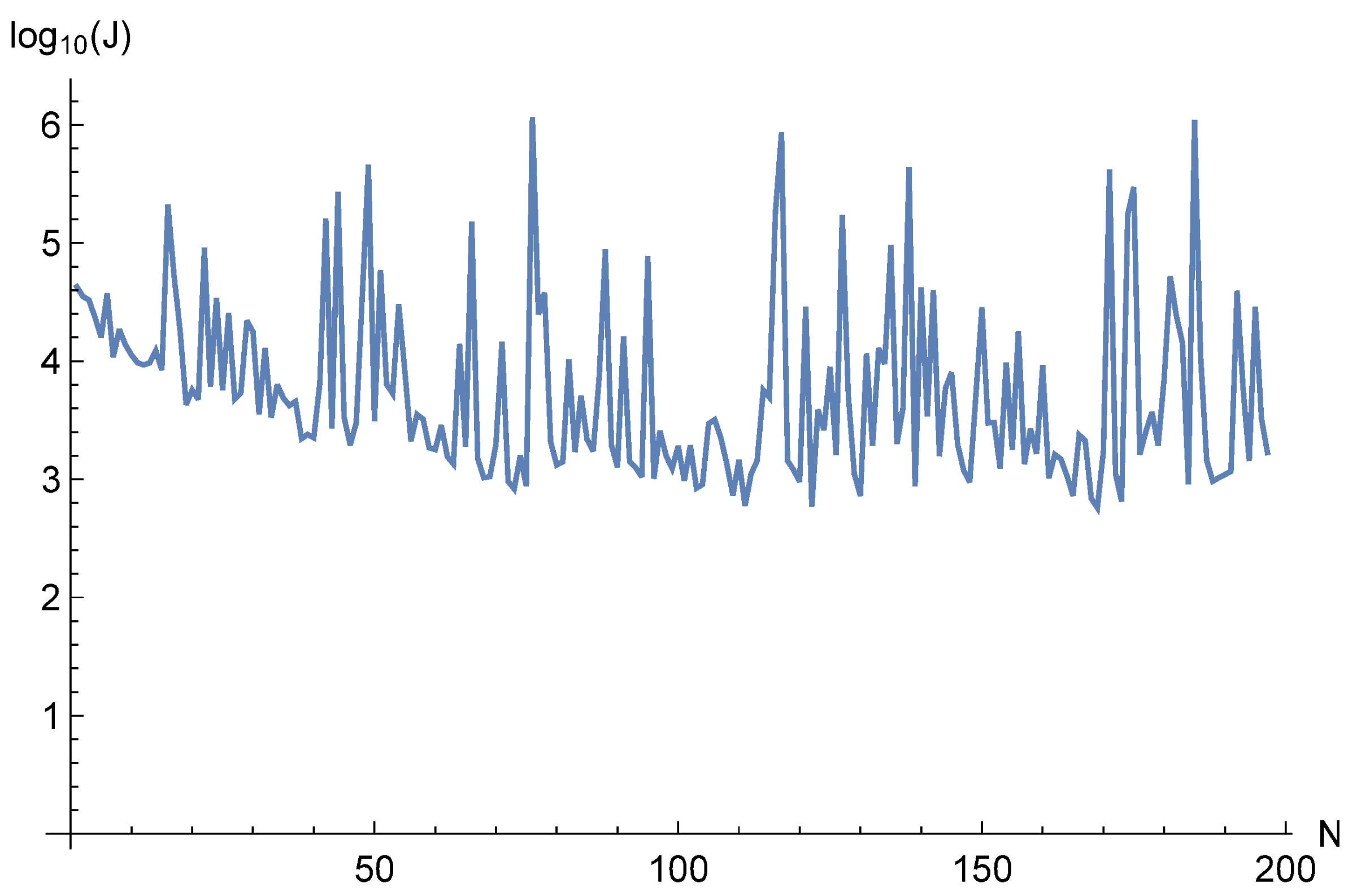
We had previously shown (see, for example, [
15]) that the optimal number of steps in the learning process between point regeneration is from 3 to 5. In addition, this approach allows us to control the quality of training using standard statistical procedures. In this way, the number of sample points can be significantly reduced without compromising accuracy [
29]. At the same time, the learning process becomes more stable and does not get stuck in local minima. In fact, not one function but a sequence of functions is optimized, and each is a discrete approximation to the integral form of the loss function.
If the model must satisfy additional conditions, for example, measurement data , a term is added to the loss function. Thus, , where .
We have dedicated a number of works to the study of modeling problems using physics-based neural networks, see [
10,
11,
12,
13,
14,
15,
16,
17,
18,
19,
20,
21,
22,
23,
24,
25,
26,
27,
28,
29,
30]. A detailed description of the methods can be found in [
29]. In recent years, physics-based ML modeling methods have included different types of neural networks. Ref. [
11] considers recurrent neural networks and applies physics-based regularization. Ref. [
31] solves the problem of modeling non-linear dynamical systems described by partial differential equations without initially given training sets. They utilize data generated on the basis of equations to train auto-regressive networks.
Note that the FEM can be regarded as a special case of the RBF network method (ELM). Most often, when using the FEM, piece-wise linear approximation is applied. In this case, triangulation is performed; that is, the domain is divided into triangles (the boundary is approximated by a broken line) and a linear function is constructed on each triangle. On the boundary of the triangles, the functions are continually joined. To obtain a representation of the solution in the form of an expansion in basis functions (
2), one can consider the behavior of the function along the rays emanating from a certain center
. In the two-dimensional case, we have
, where
are the polar coordinates of the vector
, and
is the current point. If the position of the boundary of the support of the basis function relative to its center is characterized by some function
, we can utilize
, where
. In this case, for the polygonal boundary, we obtain a piecewise linear function, for which
is calculated from the polar equations of the corresponding straight lines, i.e., at the corresponding intervals of the variation of
we obtain
. If we want the basis function on the boundary to have a zero derivative, we can use
. For a basis function of the form
, we obtain a smooth vertex. Some more complicated form of a basis function allows obtaining a smooth surface with a polygonal base, but we will not go into that.
In the multidimensional case, we can use , where and is a vector on the unit sphere, which can be parameterized by the corresponding coordinates.
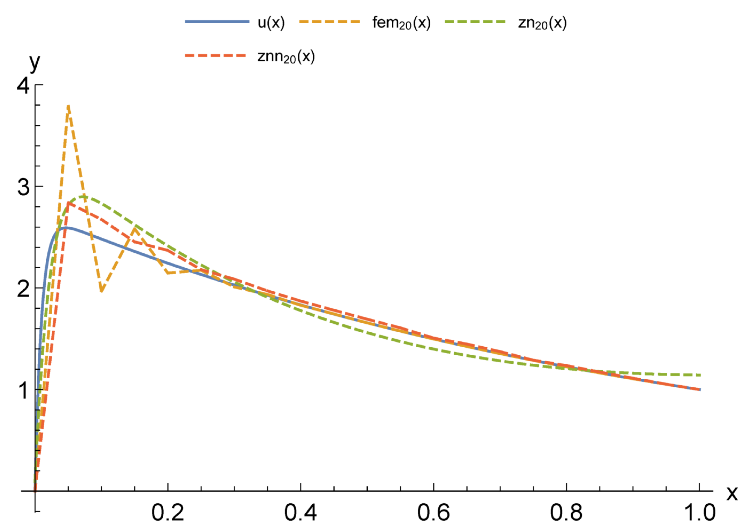
2.3. Physics-Based Neural Network Approach with FEM Smoothing
Both physics-based models considered, the FEM and ML with physics-based regularization, have their advantages and disadvantages. Higher degrees of polynomial elements lead to an increase in the cost of computation, although we obtain a solution with higher smoothness. In any case, it is not possible to obtain a solution of infinite smoothness as for neural networks.The FEM is long and more extensively applied. It is implemented in numerous commercial software products. However, the FEM using piecewise linear functions leads to an insufficiently smooth solution. In addition, if the number of elements of the method is small, the accuracy is not high enough; if it is large, the system of linear equations may require large computational resources even with a sparse matrix of system (
4).
The FEM is poorly suited to solving problems in which additional data are used to build a model. This is especially the case for tasks in which the model must adapt to the newly received data, taking into account changes in the modeling object. This is largely due to the local nature of the basis functions, which leads, in turn, to a local restructuring of the solution when trying to adapt it by minimizing the loss function . The neural networks, by their nature, are capable of being used in the problem of adapting a solution to new data. This is evidenced by the extensive utilizing of neural networks to extract the information hidden in noisy data. However, the direct application of the above neural network approach often leads to a computationally complex problem of non-linear optimization. If only parameters of a neural network solution are adjusted, a system of linear equations with a dense matrix is obtained, which dramatically increases the complexity of its solution. A more efficient approach is to first optimize the loss function , and then train the neural network when new data arrive by minimizing . However, this method is also very resource-intensive.
Alternatively, we propose the following hybrid approach. First, a solution to problem (
1) is constructed using the FEM. Further, this solution is smoothed by means of a neural network. For the approach discussed above, all the basis functions except one are equal to zero at each nodal point, and this type of model is the easiest to build. It consists of optimizing
in which the values of the FEM solution at the nodes are used instead of the measurement results. The neural network approximate solution obtained can be adapted to the newly received data in the same way as described above. Let us emphasize that in this hybrid model several physics-based modeling classes are combined.
In [
32], a FEM solution is also used as training data in the problem of structural damage identification. However, in that work, the values at nodes are not used directly, but the loss function includes two terms with the corresponding weight factors. The first is responsible for a cross-entropy loss and the second corresponds to normalized damage probabilities.
2.4. Physics-Based Multilayer Network Architecture Method
The expressions of approximate solutions constructed by using the above methods are rather cumbersome. If we write them out analytically, they turn out to be poorly visible. Much more compact approximations are obtained through an approximate series expansion or various kinds of asymptotic methods [
33]. However, these methods make it possible to build an acceptable solution only in a sufficiently small neighborhood of the point at which the expansion is constructed or for sufficiently small values of the parameter over which the expansion is carried out. In [
24] we propose another approach, which has an essentially broader area of applicability. From the point of view of the modern modeling classification, we can attribute this method to physics-based network architectures. The resulting analytical models are fairly compact.
Let us consider the initial value problem
Using the replacement, one can go from a higher-order system to a first-order multi-dimensional problem
To solve (
12), many numerical methods have been developed [
34]. A significant part of them consists of the partition of a given interval by points
into intervals of length
and applying the recurrence formula
where operator
F defines a specific method. If in (
13) the function
F depends on
, it is necessary to accurately or approximately solve (
13) with respect to
.
Applying formula (
13) iteratively
n times to an interval with a variable right end
we obtain function
, which can be considered an approximate solution of system (
12). Let us underline that, in this case,
For constructing multilayer solutions, we can choose one of the classical numerical methods [
34], for example:
the implicit Euler method, where
the trapezium method, where
the midpoint method, where
or one of many other methods of this kind.
If function is a neural network (for example, it was obtained by modeling some related process), the result is an arbitrarily accurate solution to the original problem. In this case, we refer the entire modeling procedure to the hybrid methods mentioned in the Introduction as the embedding approach. Otherwise, it can be approximated by a neural network (for sufficiently wide classes of functions, this can be done with arbitrarily high accuracy) and the equation can be solved with the replacement of the right-hand side by its approximation.
The resulting models can be regarded as physics-based pre-trained multilayer networks, the numerical parameters of which can be further trained using measurement data.
Let us consider the boundary value problem
Here, vectors and are composed of the coordinates of vector ; their total dimension is equal to the dimension of .
The following approach turned out to be an effective way to solve this problem. We choose arbitrary point
and build a solution to the system
where parameter
is adjusted based on the boundary conditions
Parameter t remains undefined. It can be chosen so that a solution satisfies the original system with the highest accuracy. For the problems of modeling real objects and constructing DT, it is more natural to adjust t based on the best fit to the measurement data.
These multilayer models can easily adapt to new data about an object. For this purpose, we can change
t and
or only
and minimize the loss function
.
takes into account only those coordinates of
for which measurement data are available. We have also studied the adaptive properties of the multilayer model in [
35].
In [
36], another scheme for imposing physics constraints on the neural network architecture is applied. They introduce a method that converts different types of equations into linear constraints and utilize them to build the output layer of a neural network. For inequality conditions, [
36] suggests using positive definite activation functions.
3. Materials and Methods. Parameterized Problems
The formalization of parameterized problems is that some parameter
appears in the formulation of problem (
1) in that
,
,
. It is required to find a solution
for which
holds for all
from a given set.
3.1. FEM and Physics-Based Neural Network Approach
Direct application of the FEM to solving problem (
20) leads to replacing (
2) by an expansion
and system (
4) is replaced by system
As a result, we have a system of linear equations with coefficients depending on the parameter. There are three possibilities among physics-based methods to solve it. The first one is analytical. The second approach uses interval analysis. These techniques work in a reasonable amount of time only when the number of items is small. Thus, acceptable accuracy is only achieved for simple tasks. Thirdly, if the problem is solved for a sufficiently representative set of parameters, this can allow estimating a solution for the entire set of parameters. At the same time, computational complexity increases many times over, and we cannot be sure that the chosen set of parameters is sufficiently representative.
The neural network approach can also be applied to a problem with parameters. In this case, the parameters are included in the number of inputs of the neural network [
29]. We have successfully solved a number of similar tasks [
15,
16]. A modification of the neural network approach to problem (
20) consists of finding an approximate solution in the form of the output of an artificial neural network of a given architecture as sum
where weights
are determined in the process of step-by-step network training based on minimizing the loss function of the form
. Here,
and
Regeneration of points is performed as follows: first, and are re-generated from a parameter change domain and then and .
If additional data are available, for example, measurements, is added to the loss function. Here, is a measurement corresponding to the value of a required solution at point and parameter value .
Despite the natural ability of neural network models to adapt to data, the process of constructing them often has a high computational complexity.
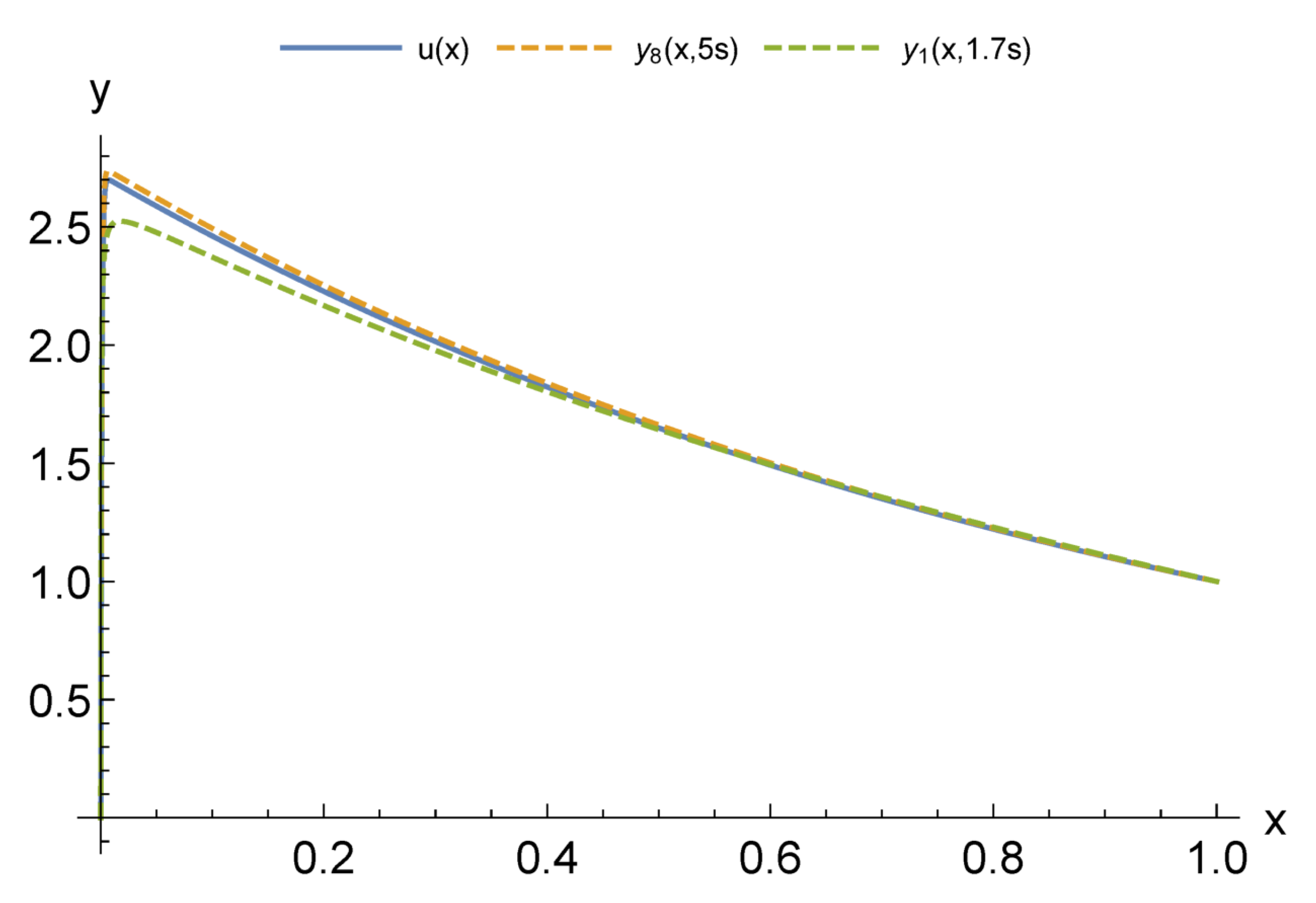
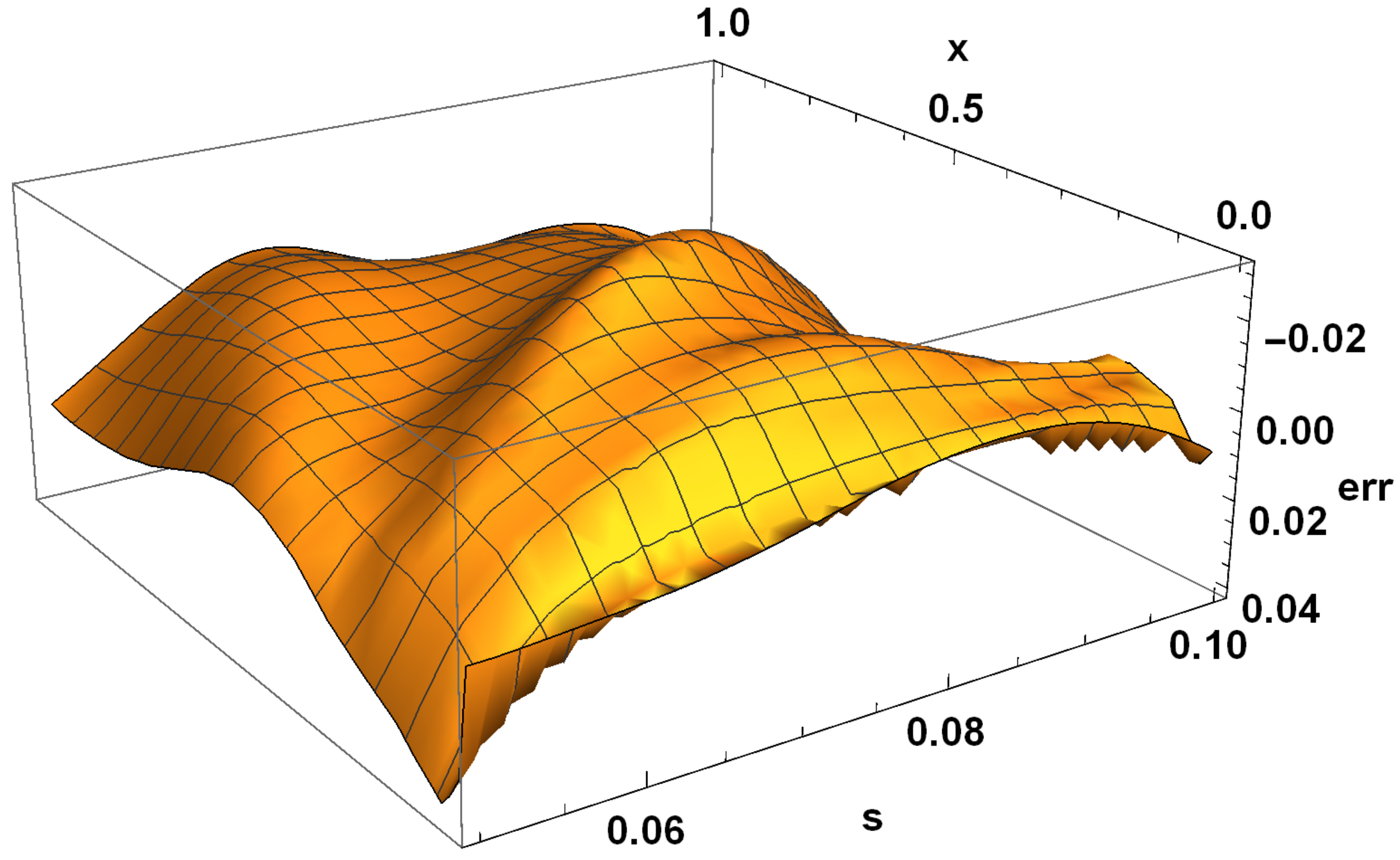
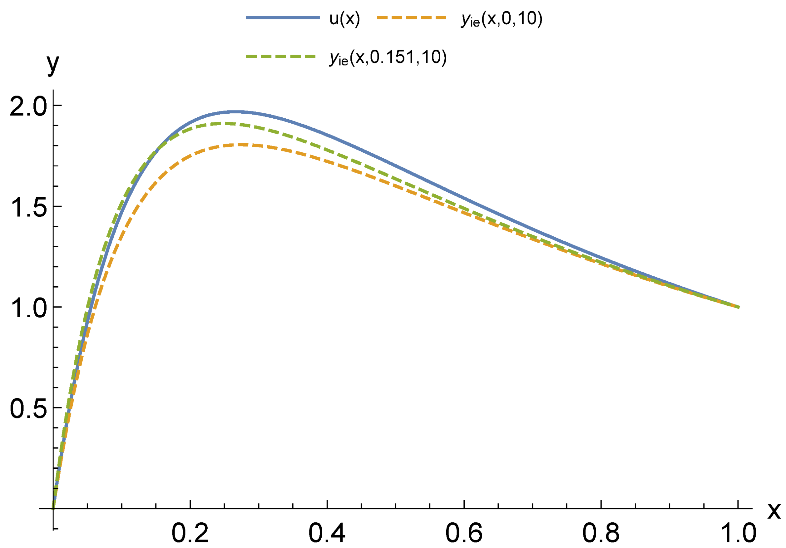
3.2. Parametric Physics-Based Neural Network Approach with FEM Smoothing
In order to combine the advantages of the FEM and neural network method for problems with a parameter, we propose the following hybrid method. Suppose we have constructed a finite element solution for a set of parameter values
Further, we construct neural network approximations for the coefficients
where
are neural network basis functions. We can apply the previously discussed RBF or perceptron-type functions. Our experience [
10,
29] shows that the latter perform significantly better in these tasks. Weights (parameters) of all neural networks are selected by minimizing corresponding loss functions, for example, in the form
The obtained solution
can be utilized not only for interpolation in the range of parameters for which the FEM was used. It is also applicable for extrapolation to the region in which the FEM solution is difficult due to the ill-conditioned matrix.
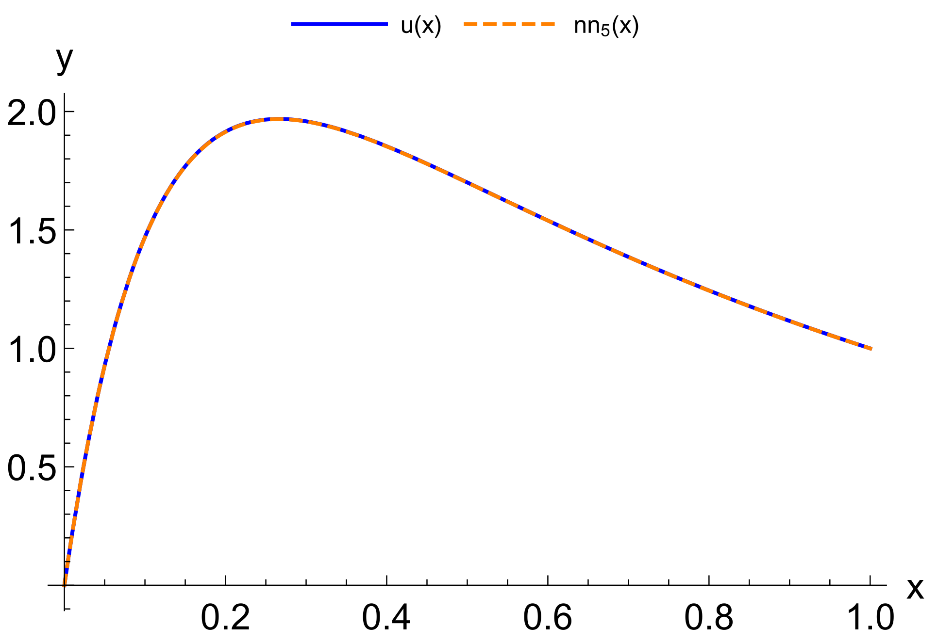
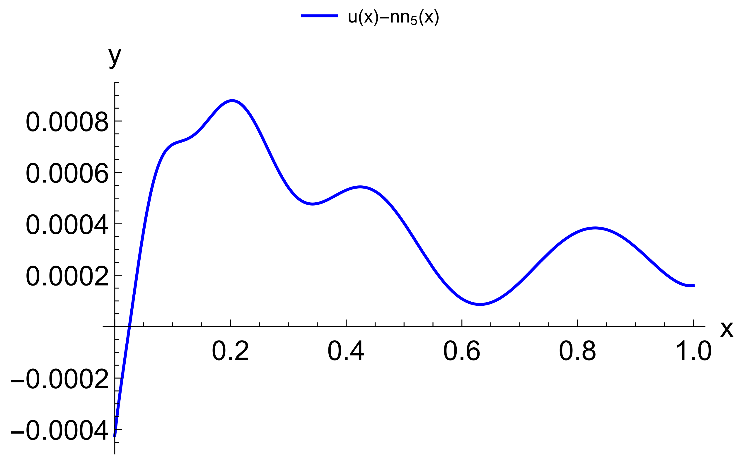
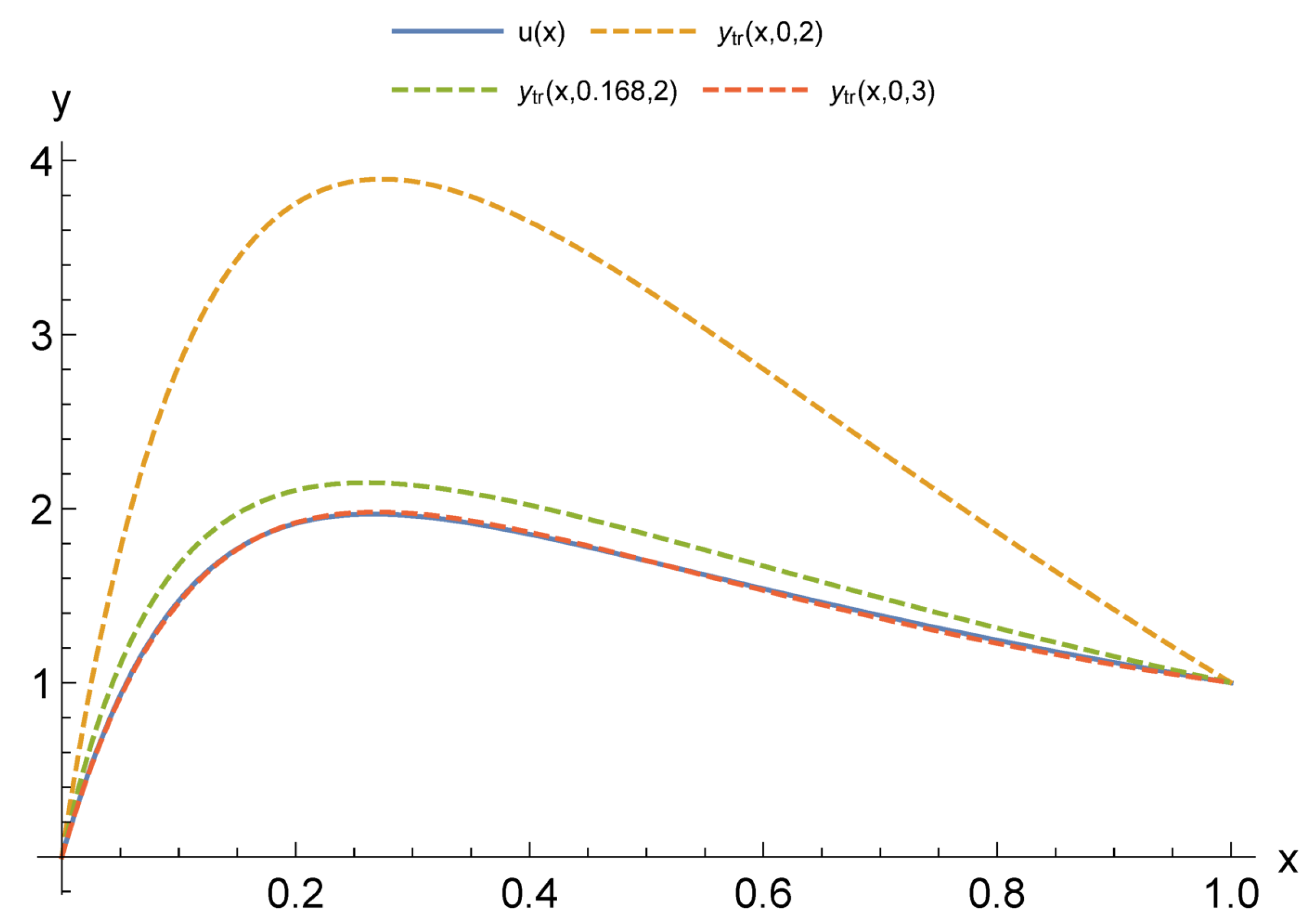
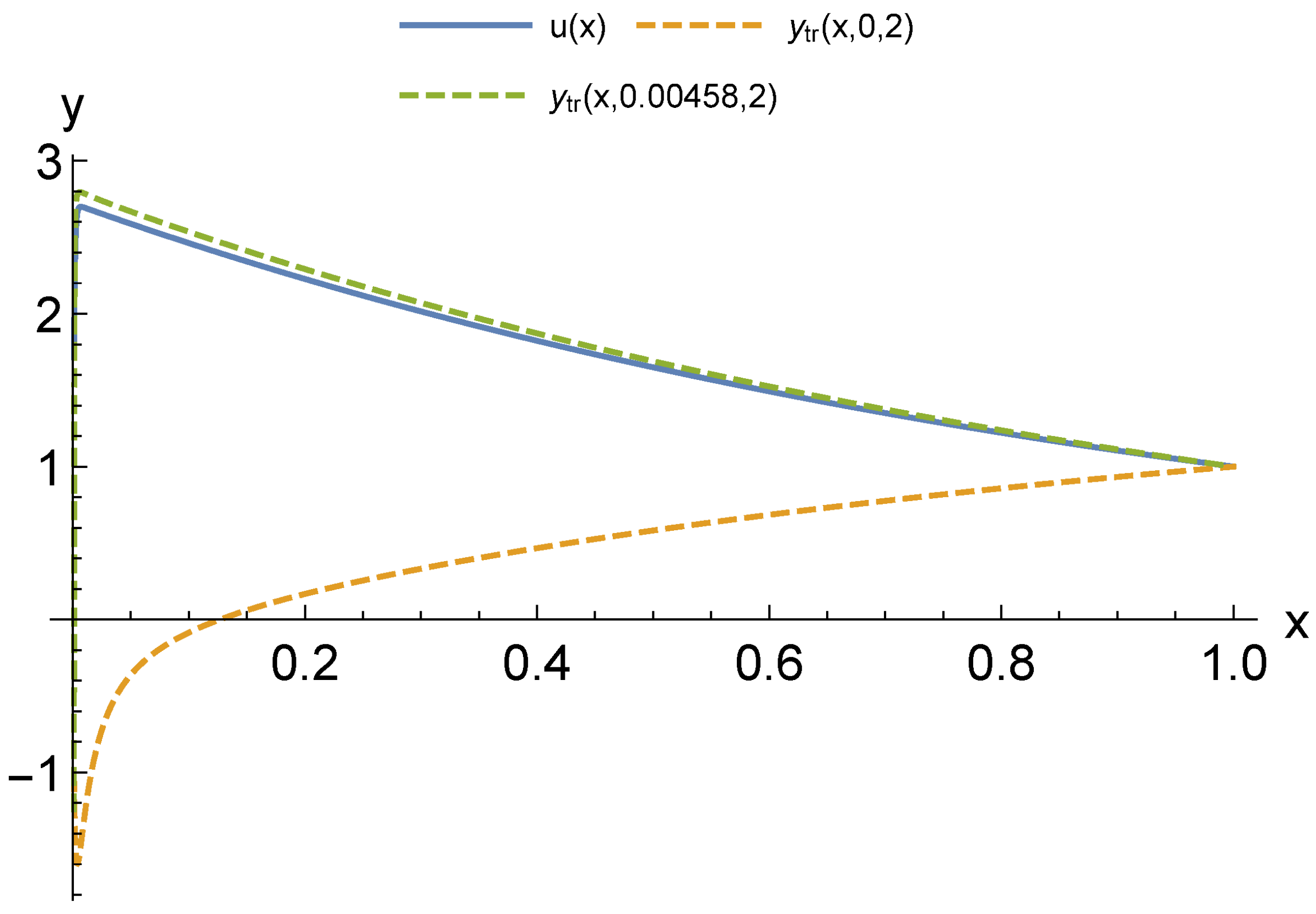
3.3. Parametric Physics-Based Multilayer Network Architecture Method
As mentioned above, in the multilayer method physics defines network architecture. This technique can be applied to solving parameterized problems virtually without any modifications.
Let us consider the Cauchy problem of the form
and apply the same recurrence formulas to it as for the problem without a parameter. As a result, we have an approximate solution
. A separate issue is the selection of dependencies
. In simple problems we can use, for example, a linear dependence on
. In tasks with measurements, we can select this dependence in the form of a neural network. In this case,
and
.
At the first stage, we again write down the formula for approximate solution . At the second stage, we adjust parameters and by minimizing the loss function .
The study of the ability of a multilayer model to learn upon receipt of additional information about an object has been started in [
37]. In [
8], an arbitrarily accurate implicit Runge–Kutta time stepping scheme with an unlimited number of stages is utilized as the basis for one of two algorithms for constructing data-driven models based on physical constraints described by general non-linear partial differential equations. In addition, the problem of the data-driven discovery of partial differential equations is solved. However, the authors acknowledge the complexity of the proposed algorithms in comparison with classical numerical methods.
5. Discussion
For modeling CPS, an urgent issue is the transition from differential models to functional ones. At the same time, an important factor is a possibility to adapt these models according to the observation data of the object. Our computational experiments allow drawing preliminary conclusions about what kind of models may be more suitable for further adaptation.
The main advantage of finite element models is that they are well studied. Accordingly, there are a large number of software packages and libraries. At the same time, with the appearance of stiffness in the problem being solved, the number of necessary functions to obtain acceptable accuracy increases sharply. Moreover, difficulties in adapting the solution increase, since it becomes unstable against data errors. This problem is aggravated by the local nature of the basis functions. Neural network models are more capable of adaptation. However, the process of their construction has a high computational complexity that also greatly increases with the appearance of stiffness. This situation allows us to look prospectively at the hybrid approaches we have considered. Even more interesting are multilayer models, which are the most compact for a given accuracy. We have already studied their adaptive properties on one problem [
37]. We intend to continue this study in further research.
Another important issue is computational costs. The fastest are multi-layered methods as they do not require training. The next ones are methods with constant basis (activation) functions but, as a result of their application, larger models are obtained. It also takes more time to adapt them further. The training of neural networks can be accelerated, but this is relevant for the stage of adaptation from measurements in real time. In the future, we intend to compare the adaptive properties of multilayer models and neural networks with different acceleration options: structure adaptation, faster methods, and the introduction of hyperparameters.
The issue of the extension of the presented results to nonlinear problems is worth specific discussion. For these problems, the advantages of the FEM are substantially leveled, since the construction of a FEM solution is no longer reduced to solving a linear system. At the same time, the complexity of building a neural network and a multilayer solution changes only slightly.


