1. Introduction
Fed-batch bioreactors allow obtaining high amounts of biomass or products for a given process time. In turn, this is related to high growth rates or production rates [
1,
2]. The application of automatic control makes possible to have enhanced productivity during the process cultivation. To this end, substrate can be regulated at a value that leads to high growth rate in order to avoid the catabolic repression of the microorganisms [
1,
2].
Control stabilisation of bioreactors by using PI-like or non-adaptive controllers is hampered by system uncertainty, mainly lack of knowledge on: structure and coefficients of the reaction rates, reaction yields, concentration of products, and inflow substrate concentration. The main uncertainty comes from the reaction rate, as its coefficients usually vary with time. In addition, the reaction yield usually varies with time as well, and there could be measurement errors for the inflow substrate concentration, and substrate and biomass concentrations [
3,
4,
5,
6]. Controlling substrate and product in fed-batch bioreactors is also hampered by these challenges [
7,
8,
9,
10]. Nonlinear and adaptive control are capable of dealing with these uncertainties, while ensuring the asymptotic convergence of the tracking error. In addition, they can handle uncertainty on biomass concentration [
11,
12,
13,
14]. Regarding this, adaptive control of continuous bioreactors is addressed in [
14,
15], nonlinear control design for fed-batch processes is addressed in [
1,
2,
9,
10,
16], and adaptive control for fed-batch processes in [
17].
In [
16] a Lyapunov-based controller is designed for a fed-batch biomass culture. It is considered that the concentration of substrate and biomass is bounded upon bounded dilution rate. The controlled output is chosen as the substrate concentration, and the desired output is chosen as the value of the substrate concentration that leads to maximum product gaseous outflow rate. The Lyapunov function
is defined as a quadratic function of the output tracking error
, and the chosen control law is of sliding type, such that the time derivative
leads to boundedness of
and
and the convergence of
to zero. However, the controller design disregards the unknown time varying nature of the control gain, the measurement noises in substrate concentration and culture volume, and also the effect of input saturation. In [
17], the so-called decoupled adaptive controller (DAC) is applied for the culture of
P. pastoris yeast. The substrate feed rate and the air flow rate are the manipulated variables, whereas the substrate and dissolved oxygen concentrations are the controlled outputs. The reaction rate terms are unknown. The controller is a combintaion of DAC and input-output linearizing control (DIOLC). The used DAC scheme consists of an application of model reference adaptive control (MRAC), and comprises updated parameters in order to provide estimates of the uncertain reaction rate terms. The matrix inversion principle is used to handle the combined effect of the two inputs. The controller was implemented on line, with adequate but improvable performance. However, the control gains are considered as accurately known in the control design, whereas the measurement noise in the state variables and the effect of input saturation are not taken into account by the control design. In [
1], an extremum seeking control scheme is proposed for optimization of the specific growth rate in fed batch processes whose kinetics are substrate inhibited. The dilution rate is the manipulated variable, whereas the gradient of the specific growth rate is the controlled variable. The gradient of the specific growth rate is estimated through a high-order sliding mode observer, whereas the specific growth rate is estimated through an exponential observer, and the substrate concentration is estimated through an asymptotic observer, using the knowledge on the substrate to biomass yield and concentrations of biomass and feed substrate. The controller design is based on a high-order sliding mode scheme, using the estimates provided by the observer and the known yield coefficient, but not the kinetic model parameters. The stability of the closed loop variables is determined through Lyapunov functions. The controller was tested by simulation, considering measurement noise, and a time varying optimum of the specific growth rate. However, the uncertainty on the yield coefficient and the measurement noise in biomass and inflow substrate concentrations and the effect of input saturation are disregarded in the controller design. In [
15], a robust adaptive controller is designed for a class of continuous wastewater treatment processes. It is assumed that: bacterial growth rates and inlet pollutant concentrations are unknown, but some upper and lower bounds are known; the biomass and substrate concentrations are unknown. The output is defined as the sum of the concentrations of the two substrates, whereas the manipulated input is defined as the dilution rate. The controller design is based on Lyapunov function, it uses the estimates of biomass concentration provided by the interval observer, and the estimates of reaction rates provided by the estimator. However, input saturation is not taken into account in the control design. In [
14], a robust adaptive controller is designed for continuous bioreactors. The biomass concentration, the biomass growth rate, and the inflow substrate concentration are considered unknown to the controller, whereas the gas production is considered known. The substrate concentration is chosen as controlled output, and the dilution rate is chosen as manipulated input. The lack of knowledge on the inflow substrate concentration implies unknown control gain. The controller design is based on Lyapunov function, and uses an arrangement of the substrate uptake rate in terms of the measured gas production in order to partially tackle the uncertainty in the biomass growth rate. Moreover, parameter updating is used in order to cope with the lack of knowledge on the control gain and yield coefficient. However, the effect of input saturation is not taken into account in the control design. In [
2], a controller is designed for a fed-batch process with dual substrate feeding and additive kinetics. The specific growth rate is the output to be controlled, and the feeding flow rates are the manipulated inputs. The biomass concentration, the working volume, the inflow substrate concentrations, and the yields of substrate to biomass are assumed known, whereas the specific growth rate is assumed unknown. The specific growth rate is estimated through a super twisting sliding mode observer, based on the known biomass concentration. The control law is proportional to biomass, and it achieves convergence of the tracking error. However, the control gain is considered accurately known and the effect of input saturation is not taken into account in the control design.
In addition to the effects of model uncertainty, closed loop performance can be severely affected by actuator saturation if it is unaccounted in the controller design, and considerable overshoot may occur [
18,
19,
20,
21,
22,
23]. In case of adaptive controllers, the stability of the closed loop system may be lost, and windup phenomenon may occur, in which adapted parameters change excessively. One possible solution is to stop adaptation during saturation moments, although this is not an optimal one [
19,
24]. One strategy used in control design for nonlinear systems with input saturation is the so-called augmented error signal (AES). It allows preserving closed loop stability and its effectiveness has been demonstrated in several mechanical systems. In adaptive controllers with AES strategy, excessive increase of updated parameters is prevented. The AES strategy is characterized by the fact that the regular tracking error is modified by adding the state of an auxiliary system which is a filter in terms of
, the difference between the constrained and unconstrained inputs [
19,
24,
25].
A pioneering incorporation of the AES strategy to Lyapunov-based adaptive control is the direct learning control scheme presented in [
24]. Therein, it is proved that the closed loop signals are bounded despite input saturation, so that excessive increase of updated parameters is avoided. In addition, the modified tracking error asymptotically converges to a compact set of small size. In case that the control gain consists of the product of an unknown constant and a known function, the uncertainty of the constant is tackled by using an updated parameter, which is used in the auxiliary system [
24]. The design procedure of the AES strategy of [
24] comprises: (i) Formulation of an auxiliary system, involving the input error
, which is the error between the constrained and unconstrained input values; (ii) use of the modified tracking error as closed loop state variable instead of the regular tracking error, the modified tracking error consisting of the regular tracking error minus the state of the auxiliary system. The main features of the resulting closed loop system and controller are: (i) The control and update laws are function of the modified tracking error instead of the regular tracking error; (ii) the modified tracking error, the regular tracking error, and the parameter updating error are bounded despite input saturation; (iii) the modified tracking error asymptotically converges to a residual set of small size. Further control designs for input constrained systems use this AES adaptive control strategy, and the closed loop system and the controller commonly exhibit the above features, see [
19,
26,
27]. Furthermore, these AES adaptive control designs incorporate other strategies, for instance: (i) Recursive backstepping approach, for handling high-order nonlinear systems (see [
19,
25,
26]); (ii) fuzzy and neural network, for approximating the unknown system nonlinearities (see [
19,
26,
27,
28,
29]); and (iii) state observers, for handling the lack of knowledge on unknown states (see [
25,
28,
29]). In [
27], an output feedback dynamic surface control is designed for an input constrained system subject to actuator failures and saturation. The unknown states are estimated through a state observer. The uncertain nonlinear terms are identified and approximated online through a Takagi-Sugeno (T-S) fuzzy system. The “explosion of complexity” is tackled via dynamic surface control (DSC) strategy. The effect of input saturation is tackled via AES strategy with auxiliary system. An updated parameter is used in order to tackle the lack of knownledge on an unknown positive constant that is the maximum value among the auxiliary signal, the desired output, the upper bound of the external disturbance, and the approximation error. However, the control gain is considered as accurately known in the control design, and the convergence region of the modified tracking error depends on the bounds of: external disturbances, system states, and model coefficients. Therefore, to achieve the convergence of the modified tracking error to a compact set of small user-defined size, such bounds must be known. Current AES robust adaptive control designs exhibit these two limitations (see also [
19,
25]).
To the authors knowledge, application of AES adaptive control to bioreactors and to systems with unknown varying control gain is overly scarce; some examples are mentioned as what follows in which other strategies as state observers and neural networks are incorporated in the controller. In [
25], a general nonlinear time-delay system of
n differential equations is considered, and a recursive output feedback backstepping is used. Moreover, the model of a two-stage chemical reactor with recirculation is considered as a particular case of the general system. The reactor model corresponds to a second-order nonlinear system, where the first state is the known output, while the remaining states are unknown. The limitation is that the controller design considers the control gain as constant and perfectly known. In [
29], a CSTR is considered, whose model corresponds to a second-order nonlinear system, where the first state is the known output, whereas the remaining states are unknown. The controller uses neural network and a high-order sliding mode (HOSM) observer. An antiwindup compensator is used, which amounts to the auxiliary system of the AES strategy. The limitation is that the control gain is considered perfectly known. In [
30], a SISO nonlinear system of
n order with unknown nonlinear control gain is considered. The unknown nonlinear nature of the control gain is tackled by using the Nussbaum function strategy. The main limitation is that the size of the convergence region of the modified tracking error depends on the unknown model coefficients and bounds.
In this study, a Lyapunov-based adaptive controller is developed for a fed-batch bioreactor in the presence of input saturation, unknown varying model parameters, output measurement noise, and unknown varying control gain, with unknown upper and lower bounds. An adaptive robust control design based on dead-zone quadratic forms is proposed for tackling the lack of knowledge on model parameters, control gain, and measurement noise. An improved robust auxiliary system is proposed for tackling the effect of input saturation, subject to varying control gain, with unknown upper and lower bounds. The stability analysis of the system under the formulated controller includes the following proofs: boundedness of the parameter updating error; convergence of the modified tracking error to a compact set of user-defined size; and convergence of the regular tracking error to a residual set of user-defined size, in the case that the input saturation eventually ceases. The main contributions of this paper with respect to closely related studies that consider input saturation are:
- -
A new auxiliary system is proposed, which is robust against varying and unknown control gain, and unknown upper and lower bounds. In contrast, in common adaptive control strategies for input saturation, the control gain is considered as constant and known in the definition of the auxiliary system (see [
25,
29]).
- -
The modified tracking error converges to a compact set whose width is user-defined, so that model coefficients, and bounds of either external disturbances, system states, model terms, and model coefficients are not required to be known. This is in contrast to current adaptive control designs for input saturation (see [
25,
29,
30]), where the width of the convergence region depends on the aforementioned bounds.
- -
The noisy measurements of the substrate and volume are considered in the control design; the imperfectly known control gain is used instead of considering the control gain as completely unknown.
- -
The asymptotic convergence of the modified error is proved by means of the Barbalat’s lemma, and it takes into account the formulated controller, which comprises the control and update laws and the auxiliary system, involving a saturation function.
The developed strategy for tackling the unknown varying control gain is a major contribution to the AES adaptive control literature.
The organization of the work is as follows.
Section 2 presents: (i) the mass balance model of the system and the assumptions, including the measurement model; (ii) the features of the control gain, including boundedness features and their proofs.
Section 3 presents the reference model and the statement of the control goal.
Section 4 presents the adaptive controller design and the determination of the boundedness and convergence properties of the closed loop state variables. In
Section 5, simulations results are presented. In
Section 6, the conclusions are drawn.
The system model and assumptions presented in
Section 2, and the reference model presented in
Section 3, are taken from previous works. The proofs of the boundedness features of the control gain presented in
Section 2 are original work of the authors, developed on the basis of the features of the state variables and model terms stated in the assumptions. The statement of the control goal presented in
Section 3 mentions the convergence of the tracking error, the model and its assumptions, and some expected convergence features of the closed loop system. This is in agreement with robust control studies where the control goal statement comprises the convergence of the tracking error and in some cases also includes some challenges of the system and expected convergence features. Thus, the original results of this study comprise: the design of the adaptive controller and the boundedness and convergence features, shown in
Section 4; the simulations, in
Section 5; the conclusions in
Section 6; the determination and proof of the boundedness features of the control gain, in
Section 2; and the statement of the control goal in
Section 3.
4. Controller Design and Stability Analysis
In this section, the adaptive robust controller is designed for the bioreactor model (1)–(3) subject to Assumptions 1 to 5, the control goal stated in
Section 3, and the input constraint (4). Some important tasks of the procedure are: (i) dead-zone quadratic forms are used instead of the current Lyapunov function; (ii) the unknown varying model parameters are parameterized in terms of the control gain, in order to tackle the unknown varying nature of the control gain; (iii) a new auxiliary system is proposed in order to tackle both the effect of input saturation and uncertainty on the control gain; (iv) a new treatment of the
term is proposed; (v) a saturation function of the modified tracking error is used instead of discontinuous functions.
For simplicity seek, the substrate Equation (1) is combined with definition (9):
where
is known, whereas
is unknown, and both are bounded away from zero, according to properties (11) to (14). Consider the modified error
, where
is the state of the auxiliary system that will be defined later. Accounting for the tracking error
yields
Combining with Equation (20) yields
. Differentiating with respect to time, yields
. Combining this with Equation (22) yields
To handle the uncertainty on
,
,
,
,
, the following Lyaunov-like function is used:
which vanishes for
. An early form of this function is reported by [
61,
62], and latter variants are reported by [
14,
63,
64,
65]. The main properties of
are:
Differentiating (25) with respect to time, yields
Combining Equations (29) and (24) and adding and subtracting the term
, yields
being
a user-defined positive constant. The term
provides asymptotic convergence of
to zero, as is shown later in the convergence analysis.
The input
(4) is expressed as
, where:
Therefore,
. Substituting this into Equation (31), yields
The term
is upper bounded according to property (14), so that it satisfies
where
is unknown, positive, and constant. Therefore,
In order to tackle the lack of knowledge on
, we define the updating error
where
is an updated parameter that will be defined later; it allows tackling the lack of knowledge on
. From the above expression,
can be expressed as
. Substituting this into (35), yields
Substituting into Equation (33) and arranging, yields
Therein, the signal
is discontinuous with respect to
, as can be concluded from (30). This would lead to a discontinuous signal in the definition of
. To remedy this, we notice from (30) that
can be rewritten as:
where
Using this property, Equation (38) can be rewritten as:
Thus, in order to counteract the effect of the term involving
, the auxiliary system is chosen as
where
is a user-defined positive constant,
is defined in Equation (32) and
is an updated parameter that is defined later, and it allows tackling the lack of knowledge on
.
Remark 9. The main differences of this auxiliary system with respect to that of [24] are: (i) it involves the saturation function , (ii) it involves the term instead of considering the control gain as completely unknown; (iii) it involves an absolute value term that includes the signal. This features are due to the robustness strategy. Substituting Equation (42) into Equation (41) and arranging, yields
The application of the robustness strategy of [
14] would imply
for
≠ 0. Definition (10) and constraint (4) lead to
= 1 and
= 0, so that
. Therefore,
< 0 and
= 0 whenever
> 0. This would imply frequent saturation in the long term, corresponding to moments when
> 0. In order to reduce this effect, an additive constant term
is incorporated in the control input:
where
is constant, positive, user-defined, and satisfies
, and its value can be selected as the value of
at initial open loop regime. Equation (44) leads to
Substituting into Equation (43), yields
In view of Assumptions 1 to 5, the term
is bounded, so that
, where its upper bound
is unknown, positive, and constant. Therefore,
In order to account for the presence of the unknown
, we incorporate the lower bound
, defined in Equation (12):
where
,
are unknown, positive, and constant. Adding Equations (48) and (49), yields
where
Remark 10. To tackle the lack of knowledge on the input gain term , a crucial task was to incorporate the lower bound in the expression of uncertain model parameters in terms of upper bounds [Equations (48) and (49)], and in the definition of [Equations (50) and (52)].
In order to rewritte
in terms of updating errors and updated parameters, we define the updating error as:
where
is an updated parameter that will be defined later.
Remark 11. The size of the vector is the same as that of , and it is not increased by the incorporation of the additive term in the control input.
The parameter vector
can be expressed as
, and
can be expressed as
. Substituting this into Equation (50), yields:
In view of Property (11), we have
. Substituting this into Equation (54), yields
Substituting into Equation (46) and arranging, yields
Thus, the control law term can be defined as
, so as to obtain
. Since it involves the discontinuous signal
, we use the property (39), so that (55) can be rewritten as:
Thus, the control law term
is chosen as:
Using (45), the control law is:
which is continuous with respect to
and
. Substituting
(57) into Equation (56), yields
The update law is chosen so as to tackle the effect of the term
:
where
is a 2 × 2 diagonal matrix whose diagonal entries are user defined positive constants. The update law for
is chosen so as to tackle the effect of the term
:
where
is user defined, positive, and constant.
Remark 12. The controller comprises: the control law (4), (58); the update law (60) with the 2 × 2 diagonal matrix whose diagonal entries are user defined, positive, and constant; the update law (61) being user defined, positive, and constant; and the auxiliary system (42). The signals involved therein are: (i) (21), (23), (30), (51), (40), (8); (ii) the desired output , provided by model (18), with conditions (19), according to remark 6.; (iii) the input error (32), which involves (58) and (4); (iv) the constants and , which are user-defined and positive; (v) the constant , which is user-defined, positive, and satisfies .
Remark 13. In the control design procedure, a new treatment of the term is proposed, in view of the lack of knowledge on and its upper bound : (i) the term is expressed as function of its upper bound [Equation (35)]; (ii) the term is expressed as function of parameter updating error and updated parameter [Equation (37)]; (iii) the update law for [Equation (61)] is formulated so as to obtain adequate time derivative of the overall Lyapunov function.
Remark 14. The resulting auxiliary system (42) involves significant differences with respect to current ones ([25,29]), and also different with respect to that of [30]: it involves a saturation function of ; it involves the updated parameter , which is function of and ; the signal is in absolute value. Remark 15. Other major features of the control design procedure are:
The modified error is used as closed loop state variable instead of the tracking error , being provided by the auxiliary system (42);
In the expression, the effect of term is tackled by means of the term by properly defining the auxiliary system;
Due to the lack of knowledge on the lower bound of , that is , is incorporated in the arrangement of uncertain model terms as function of upper bounds [Equations (48) and (49)]; and is incorporated in the definition of the unknown parameter vector [Equation (52)];
Due to the the lack of knowledge on the upper bounds of uncertain model terms, the model terms are arranged as function of upper bounds [Equation (47)]; the model terms are arranged as function of parameter and regression vector [Equation (50) to (52)]; the model terms are arranged as function of parameter updating error and updated parameters [Equation (54)]; and the update law for [Equation (60)] is defined.
Remark 16. The main features of the formulated control law, update law, and auxiliary system are: (i) The structure of the reaction rate terms, the plant model coefficients, the control gain and the upper and lower bounds of model terms are not required to be known; (ii) the known term (8) is used instead of considering the control gain as completely unknown; (iii) instead of using discontinuous signals, a saturation function of the modified error is used in the control law and the auxiliary system, and the continuous function is used in the update laws, in this way undesired input chattering and the need of using the Filippov theory are avoided.
Remark 17. When is inside the target region , = 0, so that remains constant, which is concluded from Equations (60) and (30). In turn, this contributes to the avoidance of parameter drifting.
4.1. Control Goal
Theorem 1. [Boundedness of the closed loop signals]. Consider the model (1)—(3), subject input constraint (4) and Assumptions 1 to 5, and signals (21), (23), (30), (51), (40). If the controller (58), (60), (61), (42) is applied, then: (Ti) the signals , , , , and remain bounded; (Tii) ; (Tiii) .
Proof of Theorem 1. The Lyapunov function is chosen as
where
is defined in (25),
in (53) and
in (36). Differentiating
with respect to time, yields
Combining this with update laws (60), (61) yields
. Combining this with Equations (64) and (59), yields
Arranging and integrating, yields
Hence, accounting for (26), we have
:Thus, . In view of (62) one further obtains , . In view of (25) one further obtains . In view of (63), (53), (36) one further obtains , , and consequently , .
In view of Assumption 1, and are bounded since input saturation renders bounded. Therefore, and are bounded. In view of the definition of (23), and boundedness of , one further obtains . In view of Equation (51), one further obtains . In this way, all the components of are bounded, and using Equation (58) one further obtains . This completes the proof of Ti.
We notice that Equations (66) and (62) lead to . Further using property (27), yields . This completes the proof of Tii.
From Equation (66), (62), (63) it follows that
. Hence,
Definition (36) yields . Combining this with Equation (68), yields . This completes the proof of Tiii. □
4.2. Convergence Analysis
Theorem 2. [Convergence of signals ]. Consider the model (1)—(3), subject to input constraint (4) and Assumptions 1 to 5, and signals (21), (23), (30), (51), (40). If the controller (58), (60), (61), (42) is applied, then: (Ti) the signal converges asymptotically to , where ; (Tii) if vanishes, then converges asymptotically to , .
Proof of Theorem 2. From Equation (67), it follows that . In order to apply the Barbalat’s Lemma, we need to prove that , and .
Recall that , as stated by Theorem 1. Then, it follows from Equation (30) that . Hence .
Differentiating
with respect to time, using (30), yields:
From this we conclude that
. So far, we have proved that
,
, and
. Applying Barbalat’s Lemma [
66], yields
= 0.
Therefore, in view of (30), it follows that converges asymptotically to , where . This completes the proof of Ti.
From (42)), it follows that if vanishes, then converges to zero. In this case, from Equation (23) it follows that converges to . In view of the convergence of stated in Ti, it follows that converges asymptotically to , . This completes the proof of Tii. □
The developed controller design considers a fed-batch system, with the substrate concentration as output to be controlled, and the dilution rate as manipulated input. Remarkable features of the system are: (i) the control input is constrained; (ii) the measurements of inflow and outflow substrate concentrations are corrupted by noise, which implies that the control gain is unknown and its bounds are also unknown; (iii) the biomass concentration and the reaction rate parameters are unknown, and their bounds are also unknown. The closed loop features are: (i) The modified tracking error converges to a compact set of user-defined width, which depends on neither model terms, nor modelling error, nor model coefficients nor disturbance terms; (ii) the absence of excessive increase of updated parameters is guaranteed; (iii) discontinuous signals are used in neither the auxiliary system nor the control law nor the update law. To this end, significant improvements were made in the whole control design procedure, and the resulting auxiliary system includes an additional update law, which allows tackling the lack of knowledge on the control gain. In summary, the controller design achieves the aforementioned closed loop features, it takes into account the aforementioned system challenges, and it provides an improved design procedure. This is a significant contribution to current robust control studies for input saturated systems, in special AES-based control designs.
Remark 18. The expression (65) takes into account the formulated controller, that is, the control and update laws, the auxiliary system, and the saturation functions, and the fact that it depends on neither the bounds of external disturbances, unknown system states or model coefficients. Therefore, the proof of asymptotic convergence of the modified error is valid upon these controller features.
Remark 19. The size of the convergence region , that is , is user-defined so that it does not depend on the bounds of either external disturbances, system states, or model coefficients. Consequently, such bounds are not required by the formulated controller. This is a significant improvement with respect to current AES-based adaptive controller, e.g., [19,25]. Remark 20. In the case that input constraint were not taken into account, the controller design would be based on a dead zone function of the tracking error, , featuring = 0 when the tracking error is inside the convergence set , that is, . Moreover, the updated parameters would be integrals of terms. However, the convergence of and the boundedness of the updated parameters would not be guaranteed for input constraint. Indeed, during input saturation moments, the tracking error would increase and . Therefore, the updated parameters would continue increasing and excessive increase would occur. In contrast, in the case that input constraint is handled via AES strategy (Section 4): (i) the controller design is based on a dead zone function of the modified tracking error (), instead of , where the modified tracking error is , is a filter in terms of the input error, and = 0 when is inside the convergence set , that is, ; (ii) the updated parameters are integrals of instead of terms; (iii) the function is guaranteed to converge to zero and is guaranteed to converge to despite input saturation, as stated by Theorem 2. During input saturation events, the convergence of implies that the updated parameters do not experience excessive increase. In addition, the boundedness of updated parameter vectors and is proved by Lyapunov stability theory, in the proof of Theorem 1. 5. Simulation Results
Recall that the formulated controller corresponds to the mathematical model of the fed-batch submerged cultivation kinetics presented in Equation (1) to (3) subject to input constraint (4), Assumptions 1 to 5, being the control goal and the desired output
stated in
Section 3. The control and update laws and the corresponding parameters are stated in Remark 12. At what follows, the values of
,
,
and
are generated by using the model (1) to (3) with specific parameter values, a specific form of
, and the measurement noise models (5) to (7) with specific values of measurement errors. These values of
,
, and
are used by the controller, but the
expression, the model parameters, the specific values of measurement errors, and upper or lower bounds of model parameters or measurement errors are not.
We consider
Gluconacetobacter diazotrophicus culture [
67], and we assume that an inflow is incorporated thus resulting in a fed-batch process, so that model (1) to (3) applies. The model therein is taken to the form (1) to (3), so that
. The model parameters are shown in
Table 1.
Furthermore, the particular values of the closed loop starting time
and the reference model parameters (
,
) correspond to this culture. The measurement errors are assumed as:
where
is a filtered random signal in the range [−0.2 0.2].
A no feeding phase (
> 0) is used before the feeding phase, comprising substrate consumption and biomass growth. The feeding phase (
> 0) is started when
reaches the critical value
. Recall that this strategy can be used for fed-batch bioreactors [
4,
34].
The saturation values, the parameters of the reference model, the user defined parameters of the control and update laws, and the use of auxiliary system are defined according to three cases, whereas the desired width of the convergence set is chosen as = 0.4 and , = 20 g/L and is the time when reaches the critical value .
The three different cases aims at assessing the capability of the developed controller to achieve the expected performance under different values of the desired output , the upper limit of the manipulated input , the user-defined parameters of the control law, and auxiliary system, , , the user-defined parameters of the update laws, ,, and the use of auxiliary system:
- (i).
The trajectory is obtained through the reference model (18), the parameter , and the signal : in the first case, the trajectory is a step response of a low pass filter, ending in a constant value, whereas in the second and third cases it is a combination of that of the first case, with oscillations, in order to provide high values of .
- (ii).
The signal is higher in the second and third cases compared with the first case.
- (iii).
The user-defined parameters: in the second and third cases, the values of user-defined parameters are higher than those of the first case, in order to achieve a small tracking error despite the increased complexity of the signal.
- (iv).
The use of auxiliary system: in the third case, no auxiliary system is used.
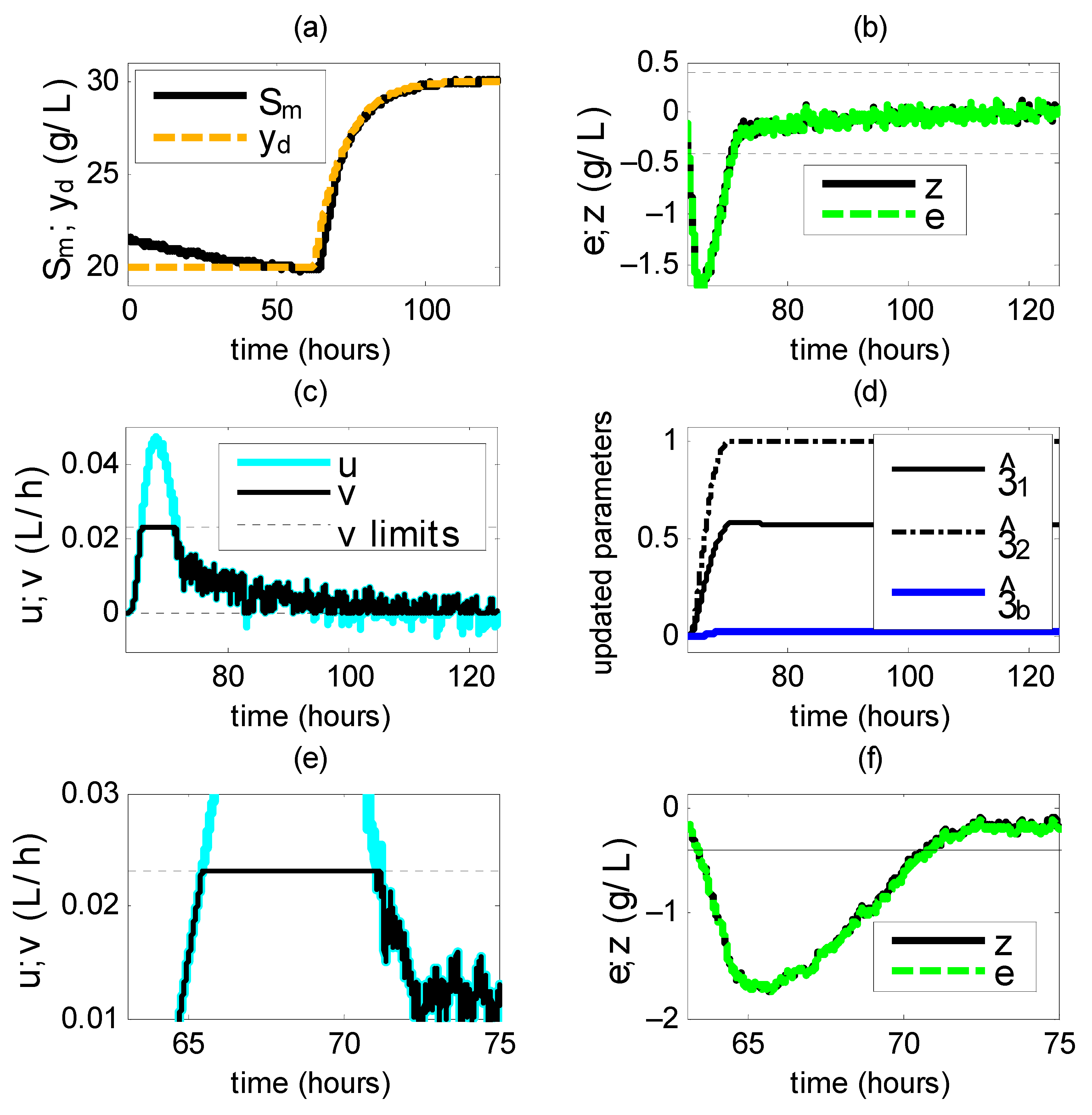
5.1. First Case
The
saturation values are
= 0,
= 0.0231
L/h. The parameters of the reference model are chosen as:
= 0.1 and
For the control and update laws we use = 1, = 0.3, = 0.1, = 0.1, = 0.01.
Simulations show that the signals
,
,
,
,
and the updated parameters
,
,
remain bounded (
Figure 1). The modified tracking error
is inside
at initial time, it is outside during [63.2 70.70] h, and it remains inside afterwards (
Figure 1b). There is an input saturation event during the time lapse [65.40 70.89] h: (i)
,
(
Figure 1b) and the constrained signal
saturates at its upper bound (
Figure 1c); (ii) the updated parameters increase, but not excessively (
Figure 1d), which is in accordance with Theorem 1. After that time period: (i)
remains in a periodic behavior with no further saturation events, so that
= 0 (
Figure 1c); (ii)
converges to
(
Figure 1b), which is made possible by parameter updating undergone before; (iii)
converges to
(
Figure 1b), which is due to the convergence of
to
and the ceasing of saturation events (
= 0) in accordance with Theorem 2; (iv) the updated parameters converge to some constant values, as a consequence of the convergence of
; in fact, they are constant when
(
Figure 1d).
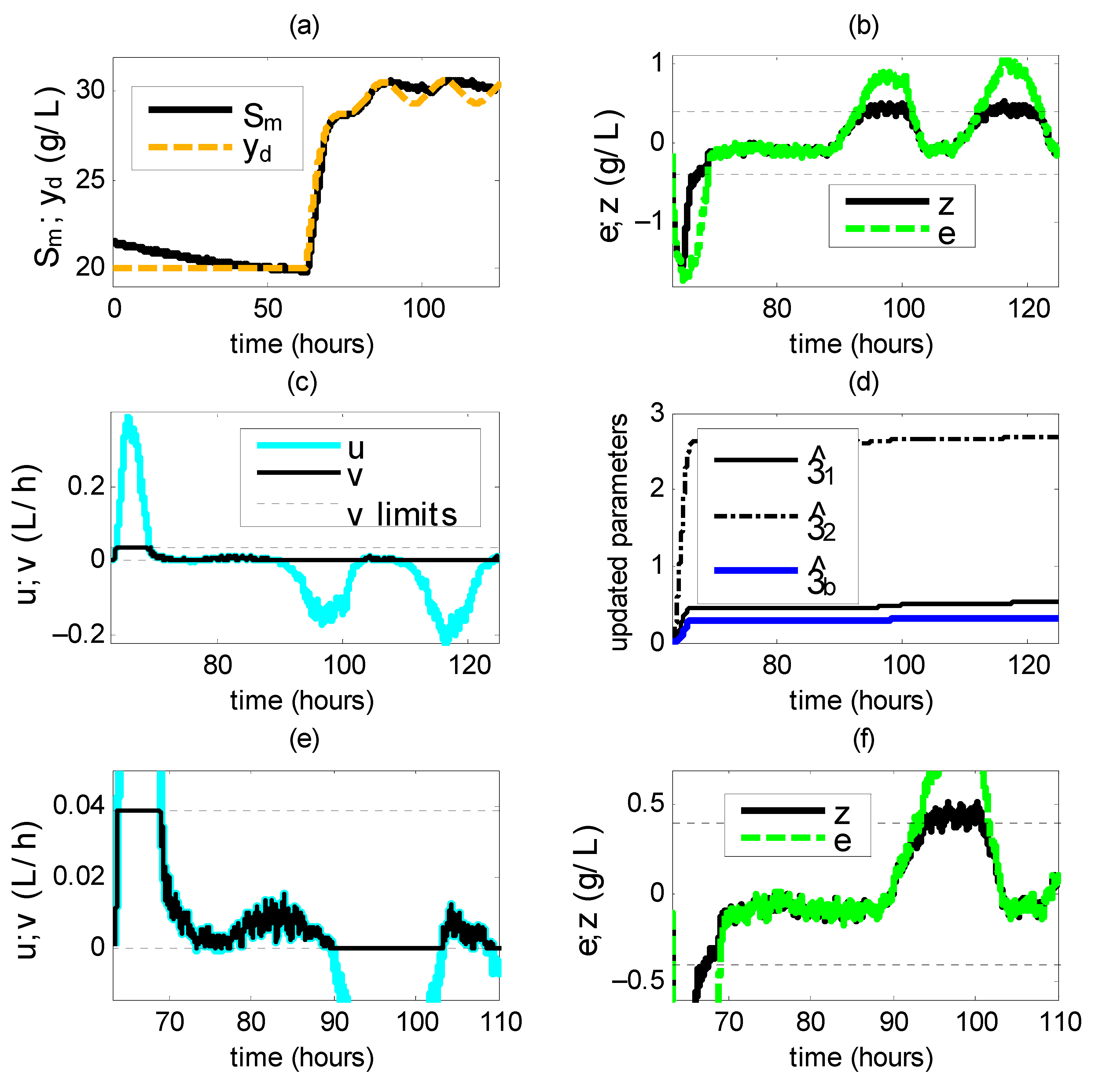
5.2. Second Case
The
saturation values are
= 0,
= 0.0385
L/h, whereas the parameters of the reference model are
= 1/5 and
For the control and update laws we use:
= 0,
= 4,
= 3,
= 0.2,
= 0.2,
= 0.2. Simulations show that the signals
,
,
,
,
and the updated parameters
,
,
remain bounded (
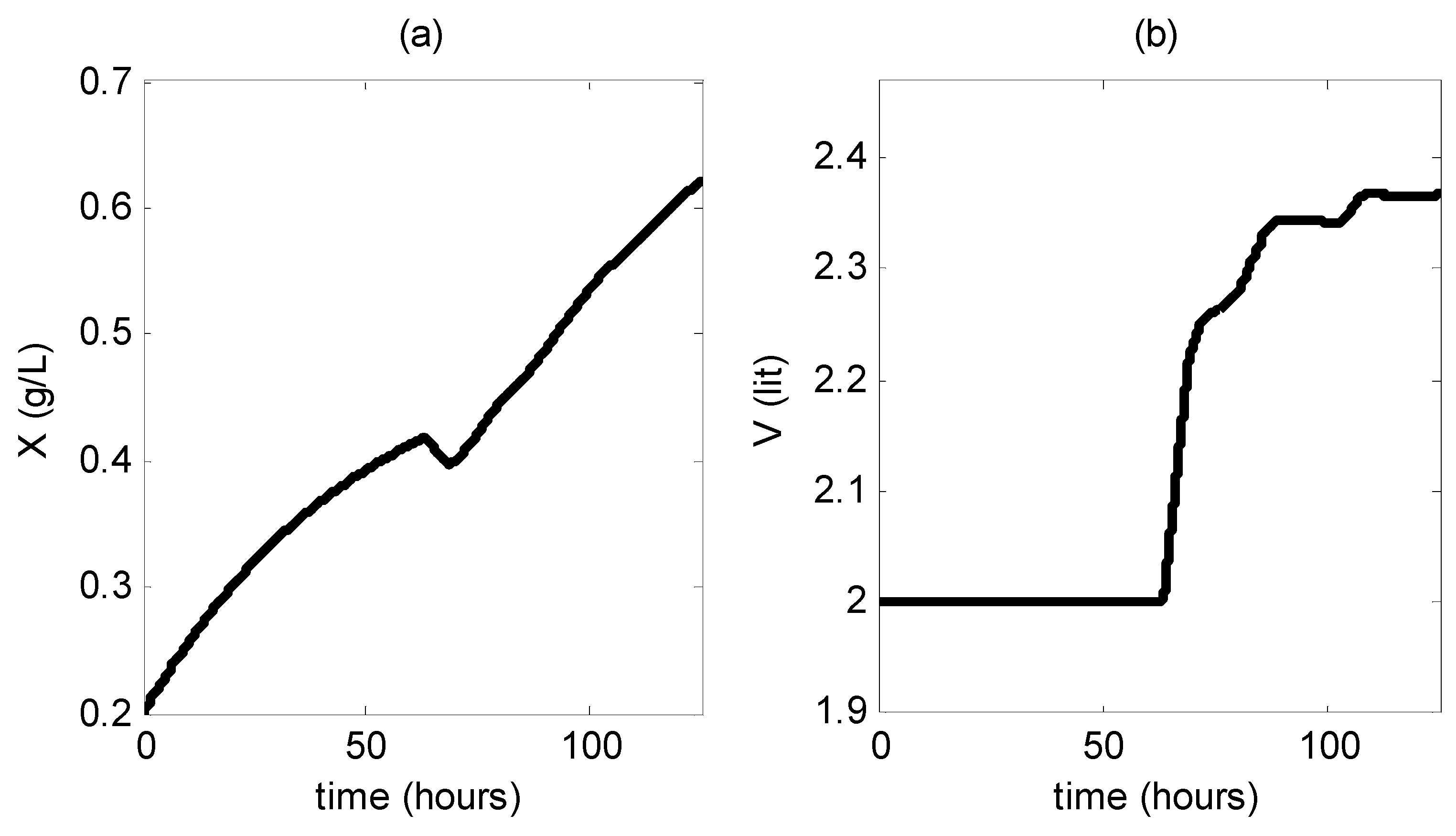
Figure 2), and the culture volume
is non-decreasing (
Figure 3). The modified tracking error
is inside
at initial time, it is outside during [63.15 67.92] h, and it remains inside afterwards (
Figure 2b). There is an input saturation event during the time lapse [63.69 69.06] h: (i)
< 0,
(
Figure 2b,f) and the constrained signal
saturates at its upper bound (
Figure 2c,e); (ii) the updated parameters increase, but not excessively (
Figure 2d), which is in accordance with Theorem 1.
After that input saturation time period,
remains in a periodic behavior with some further saturation events at its lower limit (
), (
Figure 2c,e) and
(
Figure 2b,f), which is made possible by parameter updating undergone before. Considering the whole closed loop regime, the tracking error
does not converge to
, which is due to the input saturation events. Indeed,
during input saturation events. However, it converges to a close neighborhood of
, and
during time lapses when saturation events cease, for instance during
h (
Figure 2b,f), which is due to the convergence of
to
and
= 0 during these time lapses, according to Theorem 2. The updated parameters remain constant during the time lapse featuring
, and remain unaffected by input saturation events (
Figure 2b,f).
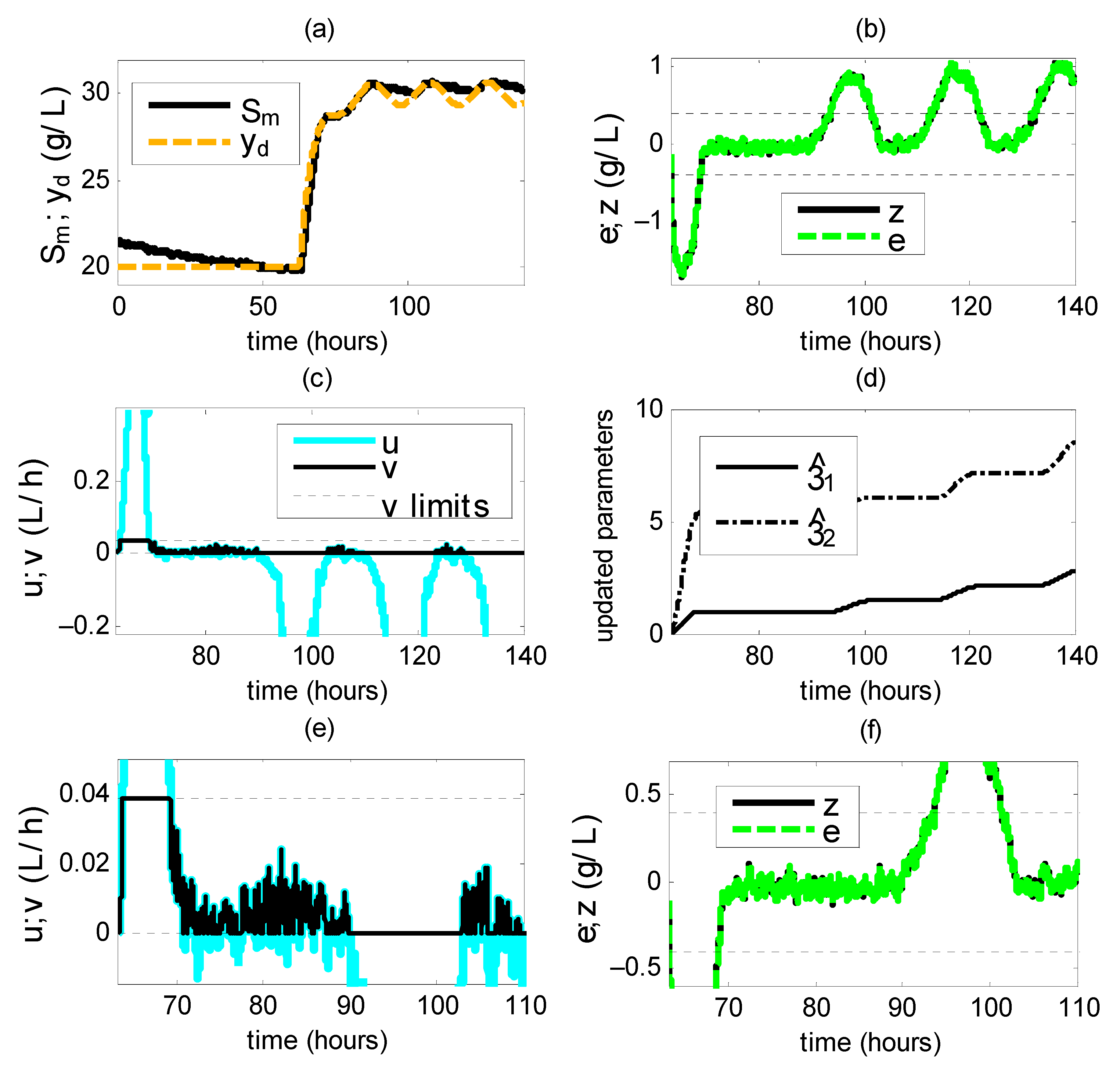
5.3. Third Case
In the third case, the saturation values (, ), the parameters of the reference model (,), the user-defined parameters of the control law and auxiliary system (, , ), and the user-defined parameters of the update laws (,) are the same as those of the second case. However, no auxiliary system is used, or equivalently, , so that is not necessary.
Simulations show that the signals
,
,
,
,
remain bounded but not the updated parameters
,
(
Figure 4). The modified tracking error
is inside
at initial time, and it exhibits intermittent dwelling periods inside
but it does not converge to
(
Figure 4b). There are several input saturation events after 89 h, during which: (i)
,
(
Figure 4b,f); (ii) the constrained signal
saturates at its lower bound (
Figure 4c,e); (iii) the updated parameters increase as
, with no upper bound (
Figure 4d). This simulation indicates us the importance of taking into account the effect of input saturation, and the effectivity of the improved auxiliary system in avoiding excessive increase of updated parameters.
5.4. General Discussion on the Simulation Results
The simulations results verify that the developed controller achieves satisfactory convergence of the modified error to the predefined compact set , with a small steady value and a small settling time, but also: the lack of knowledge on the exact values and bounds of the control gain and model terms is tackled by means of updated parameters, such that proper convergence of the signal is achieved despite this uncertainty; the effect of input saturation is tackled by means of the auxiliary system, such that convergence of the signal is achieved; discontinuous signals are used in neither the control law, nor the update law nor the auxiliary system, and saturation type signals are used instead, whereas the convergence of the signal is not affected by this fact; excessive increase of updated parameters is avoided; the tracking error converges to the user-defined residual set during periods with no input saturation.
The simulations show that the updated parameters remain constant when is inside its compact set , which verifies the effect of signal in the update laws.
From the simulations during the oscillatory behavior of in the second case for ≥ 63.2 h it follows that: (i) excessive increase of the updated parameters is avoided despite reiterated saturation events, during which the tracking error remains outside the compact set ; (ii) the tracking error converges to during periods with no input saturation ( = 0), but it is outside during periods with input saturation ( ≠ 0). In addition, the oscillations of imply that a higher control effort is required in order to achieve the convergence of the output to . To this end, higher values of controller parameters , , ,, have been used in the second case. However, the limitation of the control effort due to input saturation leads to limited speed of the output , so that it fails to reach , and the values of the tracking error are higher than required, although only during moments of higher values.


