
District-Heating-Grid Simulation in Python: DiGriPy


Abstract
:1. Introduction and Motivation
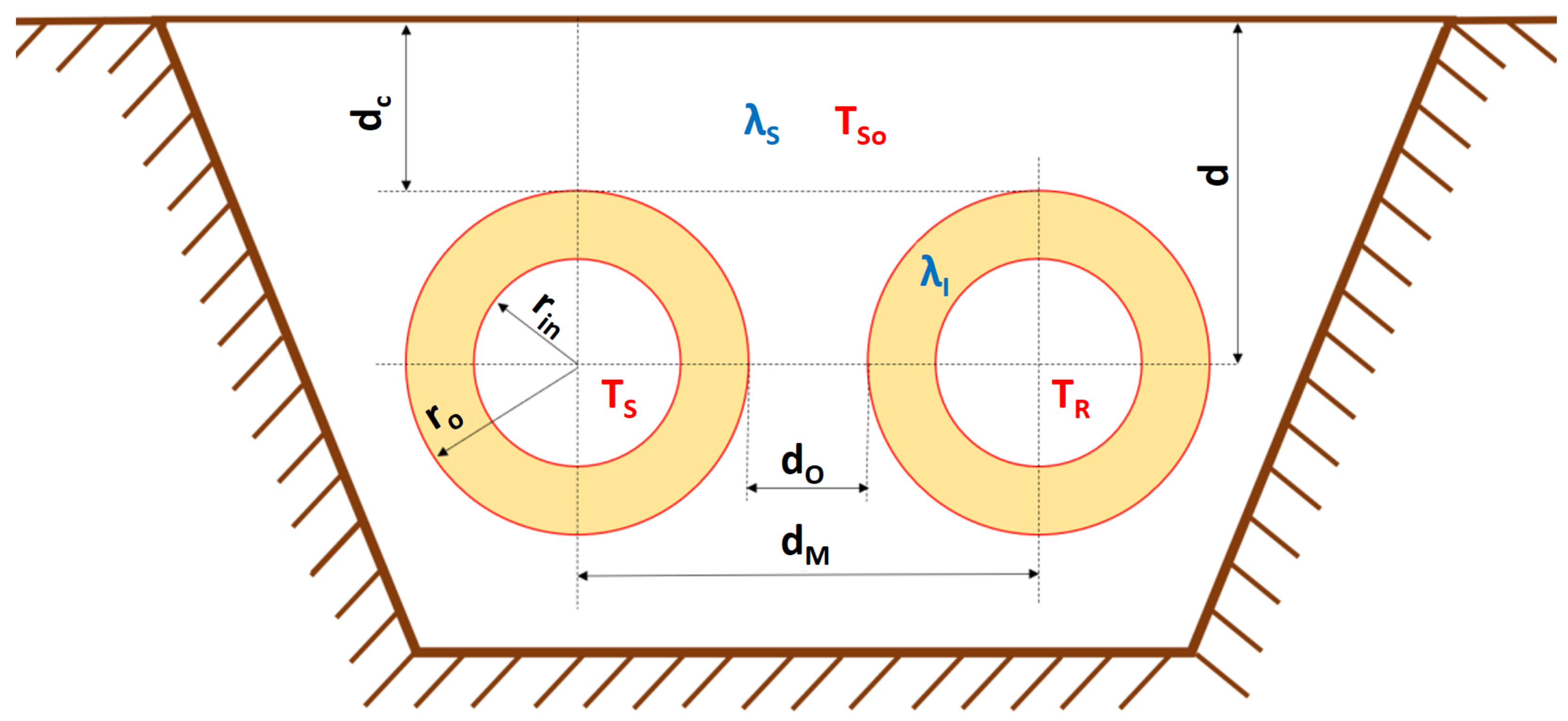
2. Tool Setup and Underlying Equations
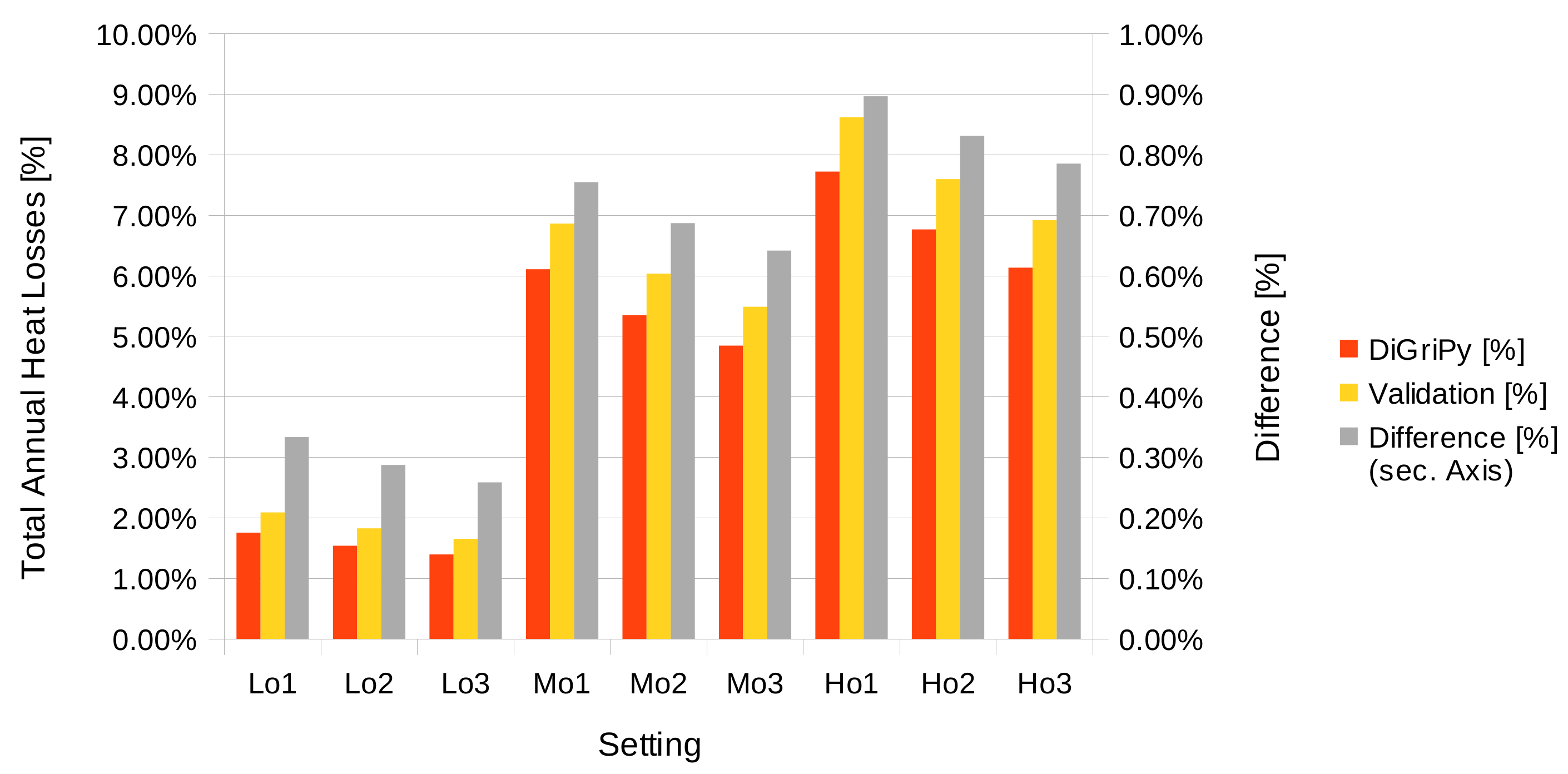
Validation
3. Implementation and Usage
3.1. Network Creation
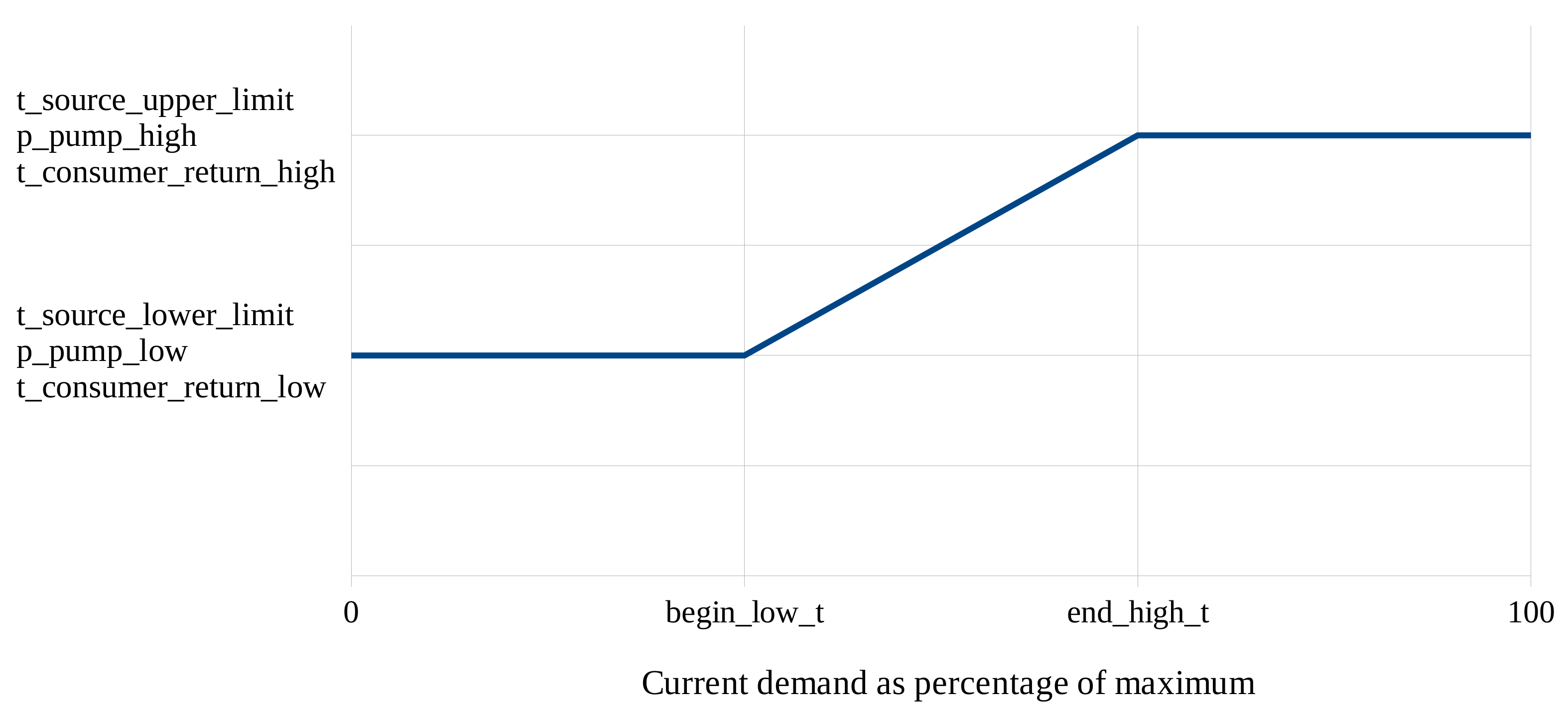
3.2. Required Simulation Input Data and Assumptions
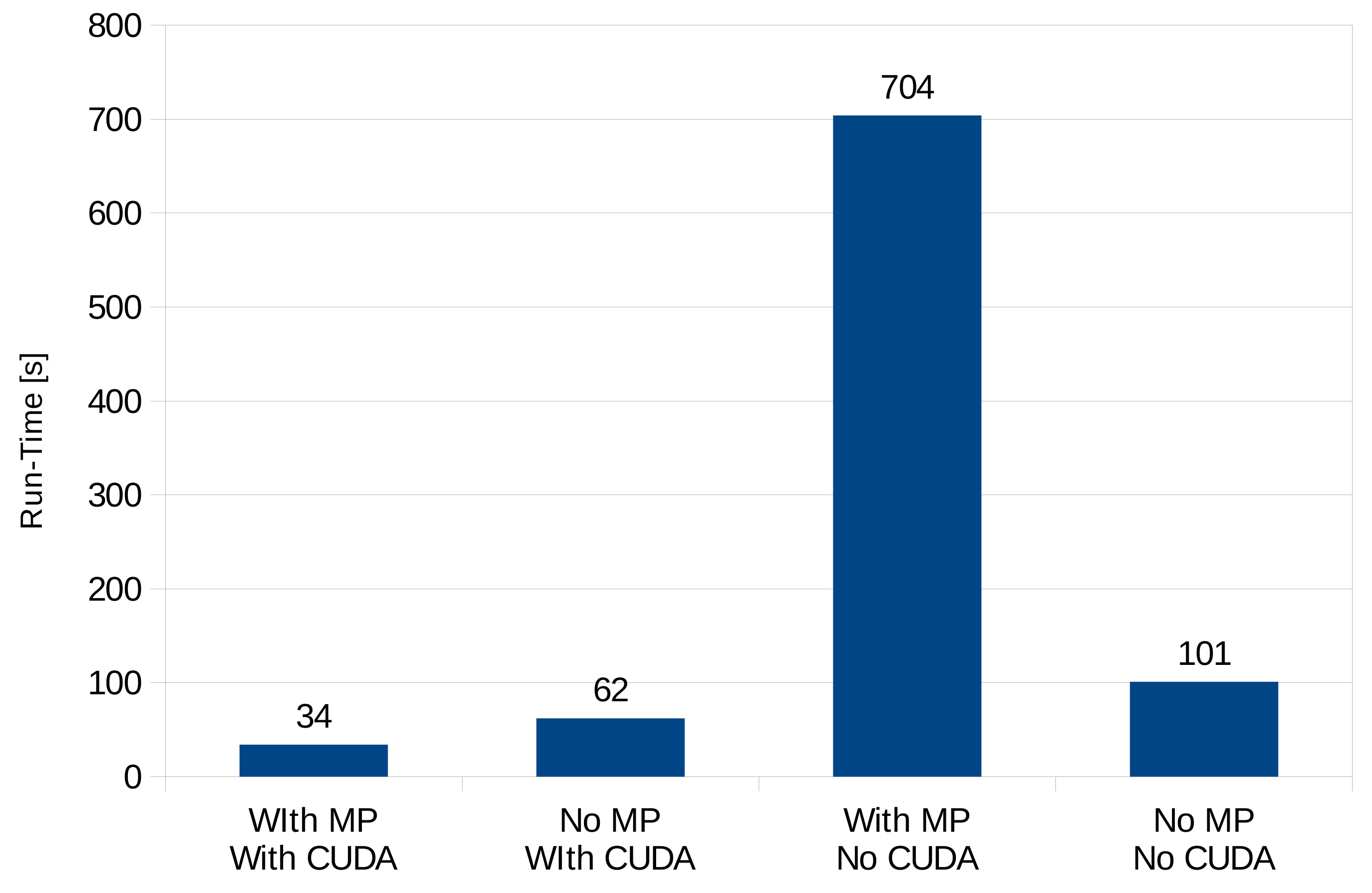
3.3. Calculation Process
3.4. Output Data
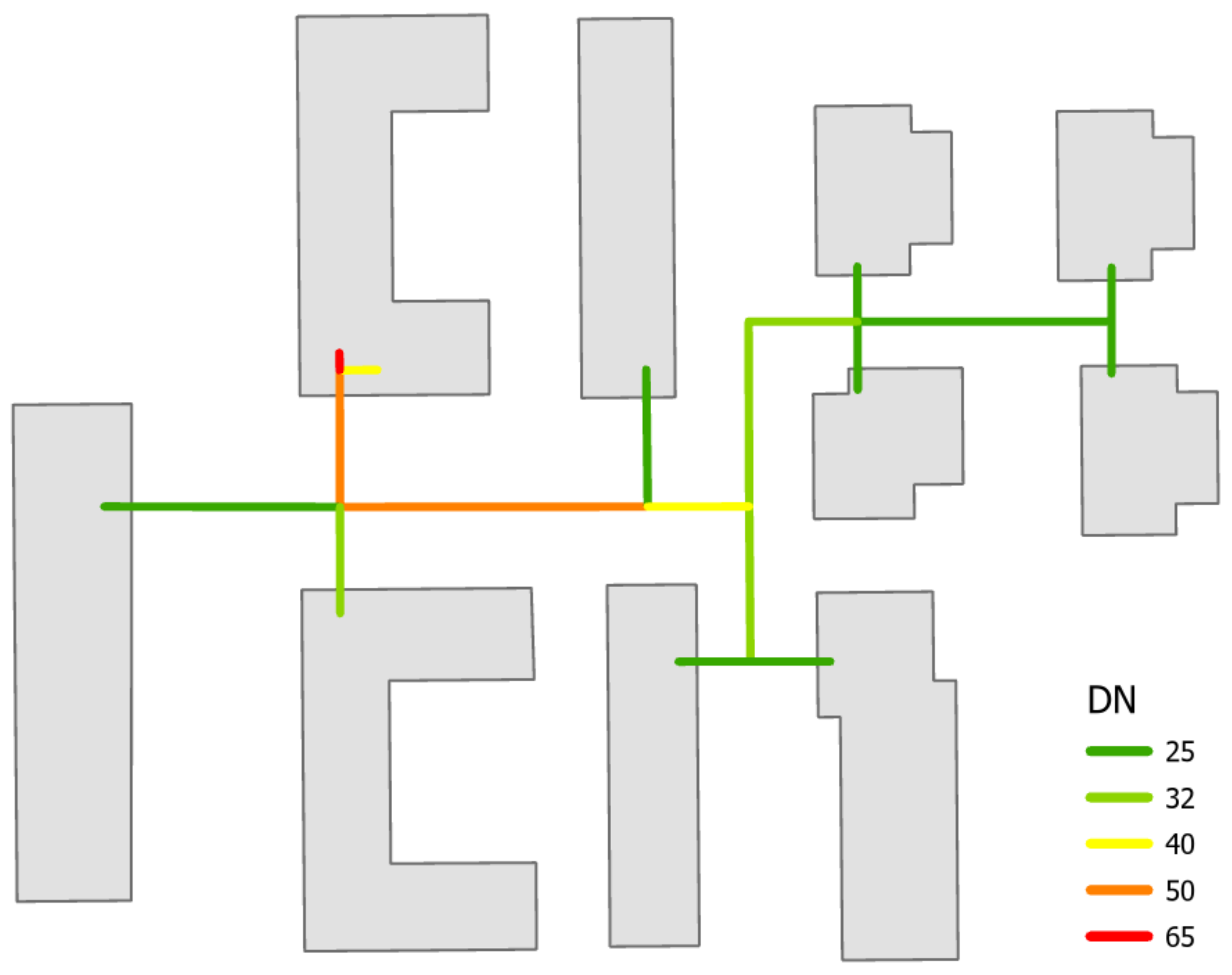
4. Test Case: Simulating a Small District
5. Conclusions and Outlook
Author Contributions
Funding
Data Availability Statement
Acknowledgments
Conflicts of Interest
Abbreviations
| CPU | Central processing unit |
| CUDA | Compute Unified Device Architecture |
| DiGriPy | District heating grid simulation in Python |
| DN | Nominal diameter |
| GPU | Graphics processing unit |
| PJP | Plastic jacket pipe |
| TESPy | Thermal engineering systems in Python |
Appendix A. Input Files

| pipe_ID | prior_ID | Passage | DN | Shape_Length |
|---|---|---|---|---|
| 1 | 0 | 0 | 65 | 2.2 |
| 2 | 1 | 1 | 40 | 4.8 |
| 3 | 1 | 0 | 50 | 17.3 |
| 4 | 3 | 1 | 25 | 29.8 |
| 5 | 3 | 0 | 32 | 13.5 |
| 6 | 3 | 1 | 50 | 39.0 |
| 7 | 6 | 1 | 25 | 17.4 |
| 8 | 6 | 0 | 40 | 12.9 |
| 9 | 8 | 1 | 32 | 19.6 |
| 10 | 9 | 1 | 25 | 9.1 |
| 11 | 9 | 1 | 25 | 10.1 |
| 12 | 8 | 1 | 32 | 23.4 |
| 13 | 12 | 1 | 32 | 13.8 |
| 14 | 13 | 1 | 25 | 7.0 |
| 15 | 13 | 1 | 25 | 8.7 |
| 16 | 13 | 0 | 25 | 32.2 |
| 17 | 16 | 1 | 25 | 6.9 |
| 18 | 16 | 1 | 25 | 6.6 |
| p_pump_low | p_pump_high | t_source_upper_limit | t_source_lower_limit | ||||
| 4 | 4 | 45 | 30 | ||||
| 4 | 4 | 45 | 30 | ||||
| 4 | 4 | 45 | 30 | ||||
| 4 | 4 | 85 | 70 | ||||
| 4 | 4 | 85 | 70 | ||||
| 4 | 4 | 85 | 70 | ||||
| 4 | 4 | 110 | 90 | ||||
| 4 | 4 | 110 | 90 | ||||
| 4 | 4 | 110 | 90 | ||||
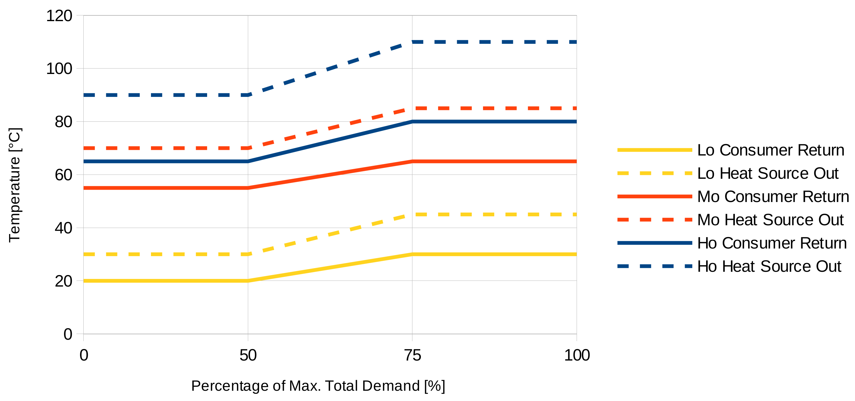
| t_consumer_return_high | t_consumer_return_low | end_high_t | begin_low_t | ||||
| 30 | 20 | 75 | 50 | ||||
| 30 | 20 | 75 | 50 | ||||
| 30 | 20 | 75 | 50 | ||||
| 65 | 55 | 75 | 50 | ||||
| 65 | 55 | 75 | 50 | ||||
| 65 | 55 | 75 | 50 | ||||
| 80 | 65 | 75 | 50 | ||||
| 80 | 65 | 75 | 50 | ||||
| 80 | 65 | 75 | 50 | ||||
| min_consumer_demand | pr_at_largest_consumer | simulate_couplings | insulation_level | ||||
| 10 | 0.6 | 0 | 2 | ||||
| 10 | 0.6 | 0 | 1 | ||||
| 10 | 0.6 | 0 | 3 | ||||
| 10 | 0.6 | 0 | 2 | ||||
| 10 | 0.6 | 0 | 1 | ||||
| 10 | 0.6 | 0 | 3 | ||||
| 10 | 0.6 | 0 | 2 | ||||
| 10 | 0.6 | 0 | 1 | ||||
| 10 | 0.6 | 0 | 3 | ||||
| pipe_type | lambda_ins | lambda_soil | depth | dist | active | t_amb | name |
| KMR | 0.03 | 1.2 | 0.6 | 0.2 | 1 | 10 | Lo2 |
| KMR | 0.03 | 1.2 | 0.6 | 0.2 | 1 | 10 | Lo1 |
| KMR | 0.03 | 1.2 | 0.6 | 0.2 | 1 | 10 | Lo3 |
| KMR | 0.03 | 1.2 | 0.6 | 0.2 | 1 | 10 | Mo2 |
| KMR | 0.03 | 1.2 | 0.6 | 0.2 | 1 | 10 | Mo1 |
| KMR | 0.03 | 1.2 | 0.6 | 0.2 | 1 | 10 | Mo3 |
| KMR | 0.03 | 1.2 | 0.6 | 0.2 | 1 | 10 | Ho2 |
| KMR | 0.03 | 1.2 | 0.6 | 0.2 | 1 | 10 | Ho1 |
| KMR | 0.03 | 1.2 | 0.6 | 0.2 | 1 | 10 | Ho3 |
| Time | 2 | 4 | 5 | 7 | 10 | 11 | 14 | 15 | 16 | 18 |
|---|---|---|---|---|---|---|---|---|---|---|
| 01/01/17 01:00 AM | 3634.7 | 6391.6 | 2986.8 | 1732.4 | 2623.0 | 7098.5 | 1448.7 | 1891.1 | 833.5 | 2234.5 |
| 01/01/17 02:00 AM | 2346.0 | 6216.9 | 2578.1 | 2248.3 | 2258.2 | 6430.2 | 1442.2 | 1683.3 | 1411.7 | 1443.1 |
| 01/01/17 03:00 AM | 2864.4 | 6232.6 | 3960.5 | 2368.7 | 2422.0 | 6795.0 | 1592.4 | 1850.8 | 1526.5 | 1657.3 |
| 01/01/17 04:00 AM | 4862.2 | 6256.7 | 3443.5 | 2558.6 | 2577.9 | 7075.2 | 1660.0 | 1990.2 | 1669.7 | 1629.0 |
| 01/01/17 05:00 AM | 5889.2 | 7730.3 | 6326.4 | 2573.6 | 5440.6 | 7902.6 | 1975.7 | 2963.4 | 1999.5 | 1970.9 |
| 01/01/17 06:00 AM | 31,325.2 | 7046.1 | 17,457.5 | 11,227.0 | 8434.4 | 8988.8 | 7793.3 | 4700.5 | 5170.1 | 10,969.9 |
| 01/01/17 07:00 AM | 77,672.5 | 10,031.2 | 29,836.5 | 11,565.4 | 17,738.6 | 17,830.6 | 9464.3 | 13,320.4 | 10,278.3 | 10,664.6 |
| 01/01/17 08:00 AM | 95,699.8 | 17,595.9 | 44,943.2 | 22,176.7 | 22,637.8 | 31,177.8 | 15,069.2 | 32,609.8 | 13,061.3 | 14,132.0 |
| 01/01/17 09:00 AM | 68,068.1 | 22,895.2 | 46,983.9 | 20,501.8 | 20,355.5 | 43,895.9 | 5963.2 | 15,744.6 | 9576.8 | 3784.8 |
| 01/01/17 10:00 AM | 65,973.5 | 16,915.8 | 27,033.8 | 22,125.9 | 18,156.7 | 49,277.5 | 6850.3 | 18,321.9 | 5926.8 | 7823.5 |
| 01/01/17 11:00 AM | 53,736.0 | 18,535.0 | 40,660.1 | 14,044.2 | 18,727.2 | 42,053.2 | 12,891.7 | 18,813.6 | 11,365.9 | 12,756.8 |
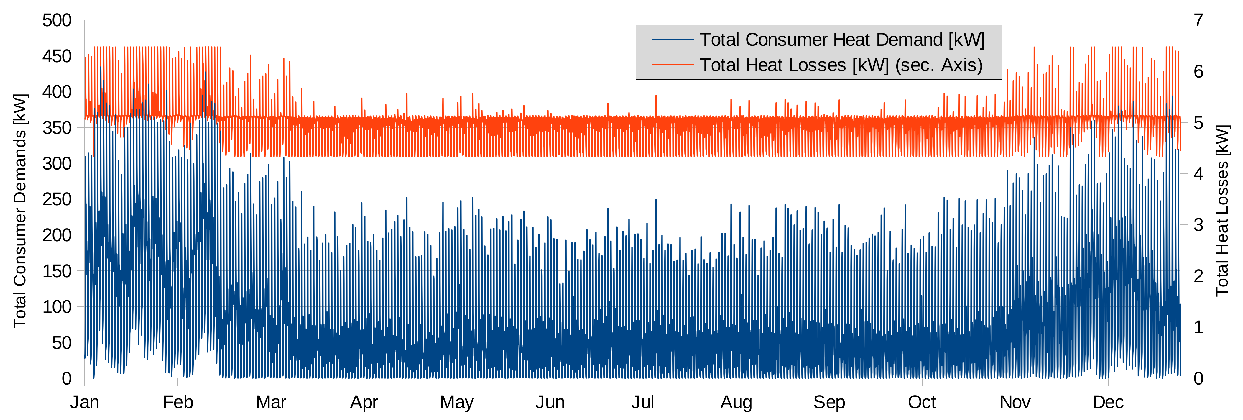
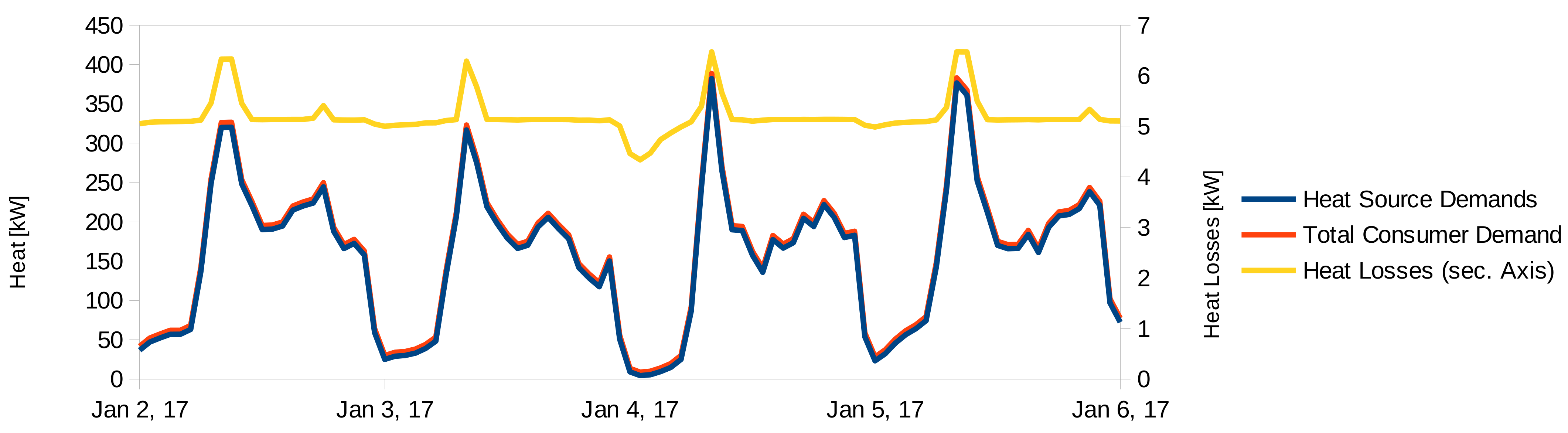
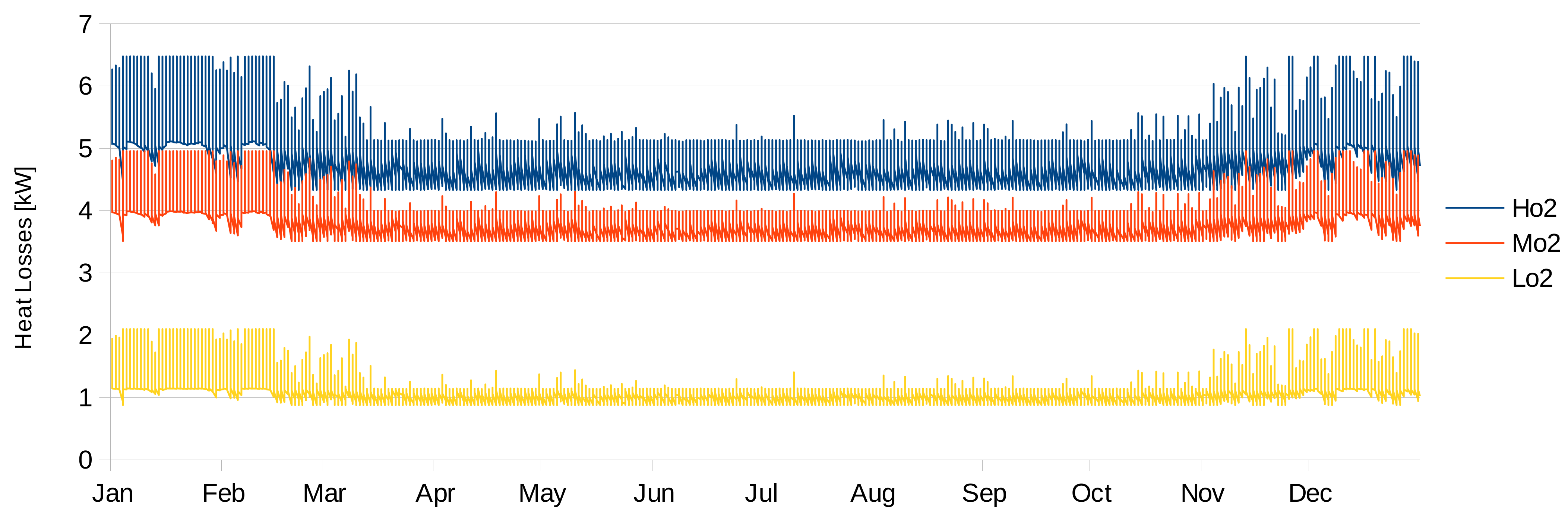
Appendix B. Demand Time Series
References
- The Paris Agreement. 2015. Available online: https://unfccc.int/process-and-meetings/the-paris-agreement/the-paris-agreement (accessed on 22 January 2021).
- Zeitreihen zur Entwicklung der Erneuerbaren Energien in Deutschland. February 2021. Available online: https://www.erneuerbare-energien.de/EE/Navigation/DE/Service/Erneuerbare_Energien_in_Zahlen/Zeitreihen/zeitreihen.html (accessed on 27 May 2021).
- European Union’s Horizon 2020 Research and Innovation Programme under Grant Agreement No. 695989. Available online: https://heatroadmap.eu/ (accessed on 30 May 2021).
- Profiles and Baselines for Heating and Cooling Energy Demands in 2015 for EU28 Countries. Available online: https://heatroadmap.eu/heating-and-cooling-energy-demand-profiles/ (accessed on 30 May 2021).
- Paardekooper, S.; Lund, R.; Mathiesen, B.; Chang, M.; Petersen, U.; Grundahl, L.; David, A.; Dahlbæk, J.; Kapetanakis, I.; Lund, H.; et al. Heat Roadmap Europe 4: Quantifying the Impact of Low-Carbon Heating and Cooling Roadmaps; Aalborg Universitetsforlag: Aalborg, Denmark, 2018. [Google Scholar]
- Ifeu-Institut, GEF Ingenieur AG and AGFW. Transformationsstrategie Fernwärme; AGFW|Der Energieeffizienzverband für Wärme, Kälte und KWK e.V.: Frankfurt am Main, Germany, 2013. [Google Scholar]
- Kobiela, G.; Samadi, S.; Kurwan, J.; Tönjes, A.; Fischedick, M.; Koska, T.; Lechtenböhmer, S.; März, S.; Schüwer, D. CO2-Neutral bis 2035: Eckpunkte eines deutschen Beitrags zur Einhaltung der 1,5-°C-Grenze. In Diskussionsbeitrag für Fridays for Future Deutschland; Technical Report; Wuppertal Institut für Klima, Umwelt, Energie: Wuppertal, Germany, 2020. [Google Scholar]
- Deutsche Energie-Agentur (dena); Allianz für Gebäude-Energie-Effizienz (geea). Szenarien für Eine Marktwirtschaftliche Klima- und Ressourcenschutzpolitik 2050 im Gebäudesektor. Final Report, Dena. 2017. Available online: https://www.dena.de/fileadmin/dena/Dokumente/Pdf/9220_Gebaeudestudie_Szenarien_Klima-_und_Ressourcenschutzpolitik_2050.pdf (accessed on 25 January 2021).
- Franco, A. Methods for the Sustainable Design of Solar Energy Systems for Industrial Process Heat. Sustainability 2020, 12, 5127. [Google Scholar] [CrossRef]
- Absatzentwicklung Wärmepumpen in Deutschland von 2012–2020. Available online: https://www.waermepumpe.de/presse/zahlen-daten/?tx_yag_pi1%5Bcontroller%5D=ItemList#yag_646 (accessed on 29 January 2021).
- Pehnt, M.; Nast, M.; Götz, C.; Blömer, S.; Barckhausen, A.; Schröder, D.; Miljes, R.; Pottbäcker, C.; Breier, H.; Nabe, C.; et al. Innovative Modellvorhaben Wärmenetzsysteme 4.0. Final Report, Ifeu, Adelphi, Ecofys, PwC, Dena, AEE. 2017. Available online: https://www.ifeu.de/fileadmin/uploads/Wärmenetze-4.0-Endbericht-final.pdf (accessed on 18 December 2019).
- ROKA3. Available online: https://www.roka3.de/ (accessed on 29 May 2021).
- NEPLAN Heating/Cooling. Available online: https://www.neplan.ch/neplanproduct/gas-water-heating-4/ (accessed on 29 May 2021).
- THERMOS-Thermal Energy Resource Modelling and Optimisation System. 2019. Available online: https://www.thermos-project.eu/home/ (accessed on 25 November 2019).
- DHNx. 2020. Available online: https://github.com/oemof/DHNx (accessed on 29 May 2021).
- Röder, J.; Meyer, B.; Krien, U.; Zimmermann, J.; Stührmann, T.; Zondervan, E. Optimal Design of District Heating Networks with Distributed Thermal Energy Storages–Method and Case Study. Int. J. Sustain. Energy Plan. Manag. 2021, 31, 5–22. [Google Scholar] [CrossRef]
- Wehkamp, S.; Schmeling, L.; Vorspel, L.; Roelcke, F.; Windmeier, K.L. District Energy Systems: Challenges and New Tools for Planning and Evaluation. Energies 2020, 13, 2967. [Google Scholar] [CrossRef]
- Nussbaumer, T.; Thalmann, S.; Jenni, A.; Ködel, J. Planungshandbuch Fernwärme; EnergieSchweiz: Ittigen, Switzerland, 2017; ISBN 3-90870505-30-4. [Google Scholar]
- Witte, F.; Tuschy, I. TESPy: Thermal Engineering Systems in Python. J. Open Source Softw. 2020, 5, 2178. [Google Scholar] [CrossRef]
- Generische Gebäudesimulation als Bestandteil der Quartier-Simulationssoftware “QuaSi”-Verbundvorhaben EnStadtEs-West: Klimaneutrales Stadtquartier Neue Weststadt Esslingen; Technical University of Braunschweig-IGS and Steinbeis-Innovationszentrum Energieplus: Braunschweig, Germany, 2020.
- Pflugradt, N.; Muntwyler, U. Synthesizing residential load profiles using behavior simulation. Energy Procedia 2017, 122, 655–660. [Google Scholar] [CrossRef]


Publisher’s Note: MDPI stays neutral with regard to jurisdictional claims in published maps and institutional affiliations. |
© 2021 by the authors. Licensee MDPI, Basel, Switzerland. This article is an open access article distributed under the terms and conditions of the Creative Commons Attribution (CC BY) license (https://creativecommons.org/licenses/by/4.0/).
Share and Cite
Vorspel, L.; Bücker, J. District-Heating-Grid Simulation in Python: DiGriPy. Computation 2021, 9, 72. https://doi.org/10.3390/computation9060072
Vorspel L, Bücker J. District-Heating-Grid Simulation in Python: DiGriPy. Computation. 2021; 9(6):72. https://doi.org/10.3390/computation9060072
Chicago/Turabian StyleVorspel, Lena, and Jens Bücker. 2021. "District-Heating-Grid Simulation in Python: DiGriPy" Computation 9, no. 6: 72. https://doi.org/10.3390/computation9060072
APA StyleVorspel, L., & Bücker, J. (2021). District-Heating-Grid Simulation in Python: DiGriPy. Computation, 9(6), 72. https://doi.org/10.3390/computation9060072