Article

Application of a Deep Neural Network to Phase Retrieval in Inverse Medium Scattering Problems

1
Language Intelligence Research Section, Electronics and Telecommunications Research Institute, Daejeon 34129, Korea
2
Department of Mathematical Sciences, Hanbat National University, Daejeon 34158, Korea
*
Author to whom correspondence should be addressed.
Computation 2021, 9(5), 56; https://doi.org/10.3390/computation9050056
Submission received: 5 March 2021 / Revised: 26 April 2021 / Accepted: 26 April 2021 / Published: 28 April 2021
(This article belongs to the Section Computational Engineering)

Abstract

:
We address the inverse medium scattering problem with phaseless data motivated by nondestructive testing for optical fibers. As the phase information of the data is unknown, this problem may be regarded as a standard phase retrieval problem that consists of identifying the phase from the amplitude of data and the structure of the related operator. This problem has been studied intensively due to its wide applications in physics and engineering. However, the uniqueness of the inverse problem with phaseless data is still open and the problem itself is severely ill-posed. In this work, we construct a model to approximate the solution operator in finite-dimensional spaces by a deep neural network assuming that the refractive index is radially symmetric. We are then able to recover the refractive index from the phaseless data. Numerical experiments are presented to illustrate the effectiveness of the proposed model.

1. Introduction

Consider an operator T 0 from a certain vector space X to another vector space Y:
T 0 : X Y x y .
The direct problem may be regarded as finding y for a given x. On the other hand, in the inverse problem, one seeks x, which represents the parameters characterizing the system, from the measurement y. In many important applications, such as signal analysis, imaging, crystallography, and optics, the space Y is defined in the complex field, i.e., y is a complex valued function such as y = | y | e i Φ . However, it is very computationally expensive or even impossible to measure the phase Φ . For this reason, the phase retrieval problem, written as
y = T ( x ) : = | T 0 ( x ) | ,
has been studied intensively and has a long and rich history in various aspects. One of the main difficulties in the phase retrieval problems lies in nonuniqueness. Consider a classical signal recovery problem that reconstructs the signal f ( t ) from the amplitude of its Fourier transform F ( f ) : = f ( t ) e i ξ t d t . Even taking into account trivial ambiguities such as translation and reflection invariance, it is known that there is no uniqueness in phase retrieval. For example, for any function g such that F ( g ) = e i Φ ( ξ ) , the amplitudes of F ( f g ) and F ( f ) are identical. Here, f g denotes the convolution of f and g. This nonuniqueness in phase retrieval can be removed by restricting the domain or property of the operator T . We refer the reader to references [1,2,3,4] for comprehensive studies on phase retrieval problems.
In this manuscript, we address the phase retrieval arising in the 2-dimensional inverse medium scattering problem, which is governed by the following Helmholtz equation:
Δ u + k 2 q u = 0 in R 2 ,
where k > 0 is the wave number and q > 0 is the refractive index. Throughout this paper, it is assumed that 1 q has compact support. That is, for a circle B R 0 centered at 0 with radius R 0 ,
q ( x ) = 1 , x R 2 \ B R 0 .
The total field u comprises the incident field u i and the scattered field u s :
u = u i + u s , u i = e i k x · d .
The incident field u i ( x ; d ) = exp ( i k x · d ) with incident direction d S 1 solves the homogeneous equation
Δ u i + k 2 u i = 0 in R 2 .
The scattered field u s satisfies the Sommerfeld radiation condition
lim r r 1 / 2 u s r i k u s = 0 , | x | = r .
The goal of the inverse medium scattering problem is to reconstruct the refractive index q from the measurement of scattered fields. This problem has been studied analytically as well as numerically in many fields, such as medical imaging, nondestructive testing, optics, radar, and seismology. See [5,6,7] for comprehensive surveys of this problem.
Our work here is especially motivated by the nondestructive testing of optical fibers. Generally, an optical fiber consists of a core surrounded by cladding material with the desired index of refraction. However, the index of refraction may be inaccurate due to manufacturing error, which would be problematic in optical communications. One testing method is to identify the refractive index profile q from the measurement of near-field data, i.e., u ( x ; d ) | | x | = R . However, it is very expensive to measure the scattered field, especially for high frequencies. For this reason, we seek the refractive index from the modulus of the full field data at | x | = R , where R R 0 , i.e., we want to solve
T ( q ) = | u ( x ; d ) | | x | = R | .
Note that from the motivation, we assume that q is radially symmetric throughout this paper, i.e.,
q = q ( r ) , r = | x | .
This problem can be categorized into the class of inverse problems with phaseless data, which have also been widely studied over the past decades (see, e.g., [8,9,10,11,12,13]). Although several results have been provided for the uniqueness of the inverse problem without phase information under certain restrictions (e.g., [14,15,16,17,18]), to the authors’ best knowledge, identification of the refractive index from the measured data set { | u ( x , d ) | : | x | = R , d S 1 } remains open. Furthermore, it is well known that the inverse problem is severely ill-posed in the sense that the solution q is highly sensitive to changes in the data | u ( x , d ) | | x | = R .
To overcome these difficulties, we invoke a deep neural network (DNN) [19] to approximate T 1 . Several works have described solving inverse problems and performing phase retrievals using DNNs. Indeed, DNNs have been shown to successfully solve various inverse problems in imaging in the last few years. We refer the reader to [20,21,22,23,24] and the references therein. In particular, there are several works that have set out to solve phase retrieval in imaging. See, for example, [25,26]. It is worth mentioning that Xu et al. proposed deep learning methods for inversion of the electromagnetic inverse scattering problem without phase information in [27]. They reconstructed piecewise constant relative permittivity profiles using the U-net convolutional neural network. In our work, we use a multilayer perceptron to train T 1 (or T ) on the subspace X M of X by considering the inverse problem as a prediction of a set of points that are Fourier coefficients of 1 q . Then, we are able to successfully construct models to approximate T 1 for various wavenumbers k. As M = 1 X M = X , it is expected that the resolution of the reconstructed q X can be increased by taking a large enough M with the proposed approach.
The rest of this paper is organized as follows: In Section 2, we discuss the direct problem for the system (1) and define the operator T , both of which are essential for obtaining the data set. In Section 3, we discretize the function spaces X and Y and redefine operator T accordingly. Then, we illustrate the numerical results with examples. Some concluding remarks are drawn in the last section.

2. Mathematical Model

In this section, we discuss the direct problem of the system (1) under assumption (2). For a general refractive index q, the solution u to the system (1) depends on the incident direction d, and they are related highly nonlinearly. However, the symmetric assumption (2) gives
u ( Q x ; d 1 ) = u ( x ; d 2 ) ,
where Q is the rotation operator such that d 1 = Q d 2 . Indeed, applying Q to x in (1) with d = d 1 yields
Δ u ( Q x ; d 1 ) + k 2 q ( r ) u ( Q x ; d 1 ) = 0 in R 2 , u ( Q x ; d 1 ) = e i k Q x · d 1 + u s ( Q x ; d 1 ) , lim r r 1 / 2 u s ( Q x ; d 1 ) r i k u s ( Q x ; d 1 ) = 0
due to the rotational invariance of the Laplacian. The uniqueness of the direct problem (1) together with e i k Q x · d 1 = u i ( x ; Q 1 d 1 ) implies that
u ( Q x ; d 1 ) = u ( x ; d 2 ) , d 2 = Q 1 d 1 .
That is, for a given u ( x ; d 1 ) , one can determine u ( x ; d ) for any d S 1 as long as the refractive index q is radially symmetric. Thus, without loss of generality, we set
d = ( 1 , 0 )
and we omit d from u ( x ; d ) and u i ( x ; d ) .
It is well known that the system of Equations (1) is equivalent to the Lippmann–Schwinger equation (e.g., [6]),
u ( x ) = u i ( x ) i k 2 4 R 2 H 0 ( 1 ) ( k | x y | ) ( 1 q ( | y | ) ) u ( y ) d y , x R 2 ,
where H n ( 1 ) is the Hankel function of the first kind of order n. Let
u ( x ) = n = s n ( r ) e i n θ .
Then, we deduce that s n solves
s n ( r ) = i n J n ( k r ) k 2 π i 2 0 r ˜ J n ( k r < ) H n ( 1 ) ( k r > ) ( 1 q ( r ˜ ) ) s n ( r ˜ ) d r ˜ , 0 r <
from substitutions of the Jacobi–Anger formula [28]
u i ( x ; d ) = n = i n J n ( k r ) e i n θ , d = ( 1 , 0 ) ,
and the addition theorem [29]
H 0 ( 1 ) ( k | x y | ) = n = e i n ( θ θ ˜ ) J n ( k r < ) H n ( 1 ) ( k r > )
into (3). Here, ( r , θ ) and ( r ˜ , θ ˜ ) are the polar coordinates for x and y, respectively. J n is the Bessel function of the first kind of order n, r < represents the lesser of r and r ˜ , and r > represents the greater. By taking into account the support of 1 q and the change of variables
ρ = k r , ρ ˜ = k r ˜ ,
we have
S n ( ρ ) = i n J n ( ρ ) π i 2 0 ρ 0 ρ ˜ J n ( ρ < ) H n ( 1 ) ( ρ > ) p ( ρ ˜ ) S n ( ρ ˜ ) d ρ ˜ , 0 ρ ρ 0 .
Here, we denote
S n ( ρ ) : = s n ( r ) , p ( ρ ) : = 1 q ( r ) , ρ 0 : = k R .
It is worth noting that (5) can be derived by the method of separation of variables, which also justifies the representation of (4) (e.g., [30]). Furthermore, one can show that the integral equation (5) is uniquely solvable in L for p L 2 [6,30]. Together with the asymptotic behavior of the Bessel functions | J n ( ρ ) | C / n ( 0 ρ n / 2 ) [31], it follows that for some constant C > 0
S n L ( 0 , ρ 0 ) C 1 n ,
which implies
n = S n ( ρ 0 ) e i n θ L 2 ( 0 , 2 π ) .
We also remark that as J n = ( 1 ) n J n and H n = ( 1 ) n H n , the uniqueness of (5) yields
S n ( ρ ) = S n ( ρ ) , 0 ρ ρ 0 .
Now, we formulate the inverse problem considered here. Let X = L 2 ( 0 , R ) and Y = L 2 ( 0 , 2 π ) , and define
T : X Y q ( r ) S ( θ ) : = | n = S n ( k R ) e i n θ | .
For a given S, we are interested in solving
T ( q ) = S .

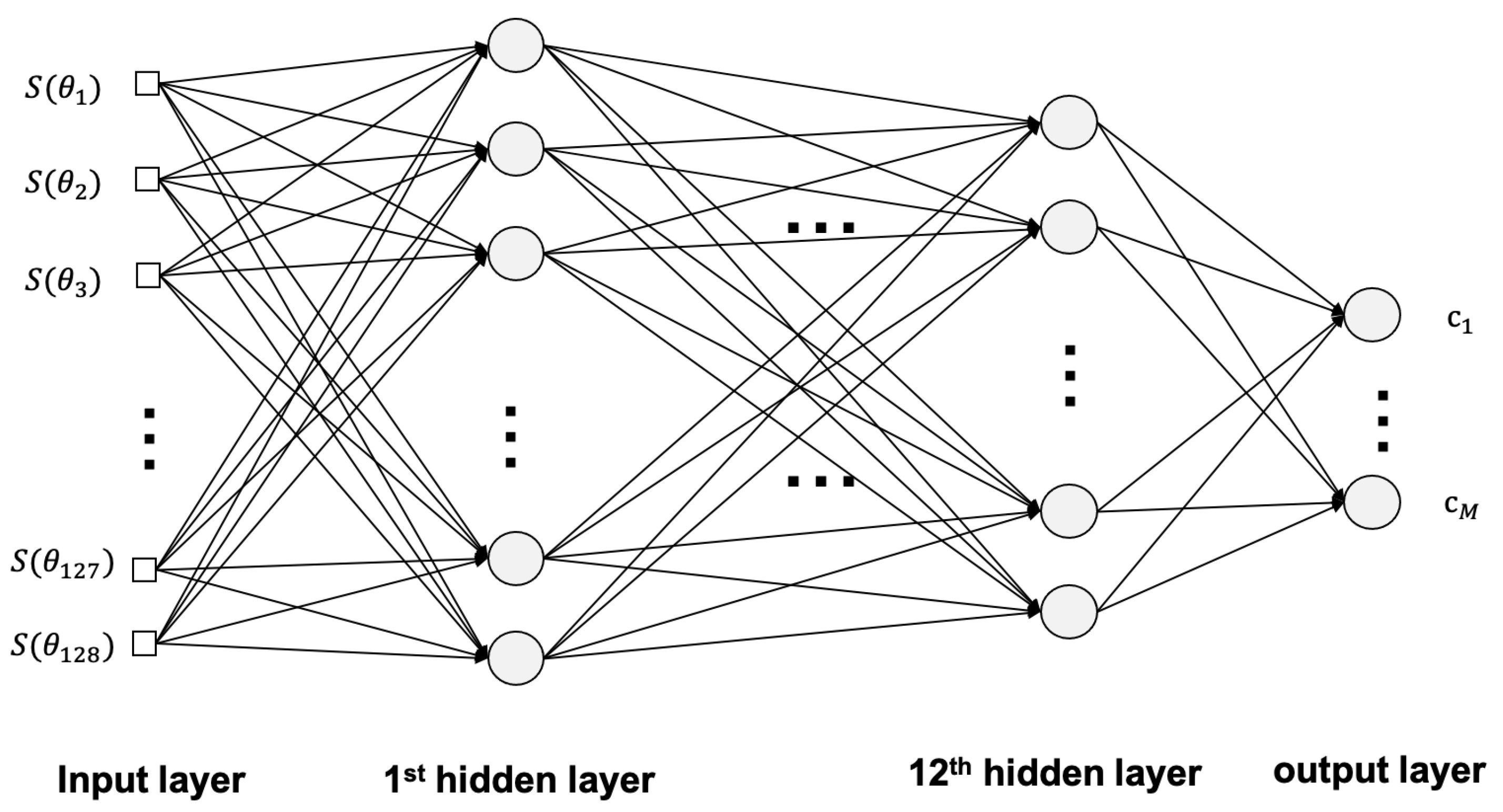
3. Deep Neural Network for the Inverse Problem

Given a set of data pairs { ( T ( q ) , q ) } , we seek to approximate T 1 with the neural network to solve (6). To this end, it is necessary to discretize q ( r ) and S ( θ ) and approximate X and Y in finite-dimensional spaces. Since it is assumed that 1 q ( | x | ) is compactly supported in B ( 0 , R ) (1b), we restrict X to square integrable functions such that q ( R ) = 1 . We further assume that q ( 0 ) = 1 to simplify the problem. That is, 1 q belongs to L 0 2 ( 0 , R ) , a set of square integrable functions vanishing at the boundary. As { sin ( m π r / R ) } m = 1 is an orthogonal basis for L 0 2 ( 0 , R ) , we approximate q ( r ) by a projectile onto X M , where
X M : = { 1 m = 1 M c m sin m π r R } .
In this manner, we are able to discretize q ( r ) as a vector C = ( c 1 , c 2 , , c M ) T . Additionally, S ( θ ) is vectorized by uniform discretization { θ l } l = 1 128 of θ in [ 0 , 2 π ] for the finite sum | n = N N S n ( k R ) e i n θ | . Here, S n ( k R ) is obtained from the numerical solution to the integral Equation (5). We use the trapezoidal rule for numerical integration to convert (5) to a linear system
S n ( ρ α ) = i n J n ( ρ α ) π i 2 β = 1 K ω β ρ ˜ β J n ( ρ α < ) H n ( 1 ) ( ρ α > ) p ( ρ ˜ β ) S n ( ρ ˜ β ) Δ ρ ˜ , α = 1 , 2 , , K .
Here, ρ 1 = 0 , ρ K = ρ 0 and ω β are weighting factors for the trapezoidal method. We take Δ ρ ˜ = 0.005 . All the computations to generate the data were performed using MATLAB R2020a.
Table 1 shows that the approximation | n = N N S n ( k R ) e i n θ | converges to S ( θ ) quickly as N increases for various q. With an abuse of notation, S denotes a column vector whose lth component is | n = N N S n ( k R ) e i n θ l | ( l = 1 , 2 , , 128 ) to represent S ( θ ) .
Now, we are in a position to approximate T 1 by
a r g m i n F Neural Net j C j F ( S j ) 2 .
DNNs have various methods such as Recurrent Neural Network (RNN), Long Short-Term Memory (LSTM), and transfer learning. However, these methods are all suitable for solving classification or time series problems. As our problem can be regarded as predicting a set of points–coefficients, we use a multilayer perceptron as our DNN. The Feed-Forward Neural Network (FFNN) is used since there is no correlation between the coefficients c i , and the network was configured according to the number of coefficients to be predicted. The architecture of a multilayer perceptron is illustrated in Figure 1. We refer the reader to references [32,33] for various methods for the DNNs.
A total of 12,000 numerical data sets with R = 1 , N = 8 , M = 5 were separated into 8000 training data sets, 2000 development data sets, and 2000 evaluation data sets. All training was performed using an NVIDIA Quadro P4000.
Figure 2 shows the distribution of relative errors of the 2000 evaluation data sets for different wave numbers, i.e., { q j q ^ j 2 / q j 2 } j = 1 2000 . Here, q is the actual refractive index and q ^ is the recovered one by the trained model. To compare the learning performance for each k, we configured the network with the same conditions each time. The network consists of 128 nodes for the input layer of sources and 12 hidden layers. The rectified linear unit (ReLU) is used for the activation function, and dropout is not adopted because it reduces the performance. We take the mean squared error for the loss function and Adam for the optimizer with a learning rate 0.00001 .
We note that in the simulations with the indicated settings, the performance of the model is low or the model is not trained for wavenumbers less than 5. This is related to the nonlinearity of the operator. Indeed, for small values of k, the scattered data are more widely distributed on { S n } than for larger k; see [11,30]. On the other hand, at high frequencies, the nonlinear Equation (6) becomes extremely oscillatory and possesses many more local minima [34]. Furthermore, the scattering data is accumulated near S 0 , i.e., | S 0 | > > | S n | for large n. This reduces the ill-posedness of the inverse problem but it also reduces the rank of { S j ( θ l ) } . Recall that S ( θ ) = n = N N S n ( k R ) e i n θ . Then, the model to be trained tends to be an underdetermined problem. For these reasons, the performance of the model at high frequency is low, as shown in the case of k = 20 .
Table 2 shows the coefficients of the recovered 1 q when q X 5 from the trained model for X 5 . The recovered coefficient c m ( m > M ) is very small in X M ( M = 2 , 4 < 5 ) , and in the case of X M ( M = 6 , 8 > 5 ) , our model acts as the projection of X M onto X 5 by ignoring the actual c m ( m > 5 ) —i.e., our model is indeed an approximation of the projection of T 1 onto X 5 . This can be verified from Figure 3 as well. In Figure 3, we show how the model can recover the refractive indexes when they are general functions that do not belong to X M . We also provide the relative errors defined as P 5 q q ^ 2 / P 5 q 2 . Here, P 5 is the projection operator onto X 5 .
One of the difficulties in solving inverse problems and phase retrieval problems is their ill-posedness; a small error in measurement may result in a much larger error in the numerical solutions. Thus, a certain regularization technique is required. The classical regularization method converts the ill-posed problem to a well-posed problem using single fidelity. On the other hand, the DNN uses group data fidelity to learn the inverse map T 1 from the training data [35]. This may also convert the ill-posed problem to a well-posed problem. Figure 4 shows how our trained model handles noise data. Indeed, we illustrate the distribution of { q j q ^ j 2 / q j 2 } j = 1 2000 in Figure 4, where q ^ is the reconstructed refractive index from noisy data S δ = S + δ with Gaussian noise δ added. We notice that the relative errors increase according to the Gaussian noise level without any sudden change. Specific examples with different signal-to-noise ratios (SNRs) are shown in Figure 5. The SNR is computed as
SNR = 20 log 10 S 2 δ 2 .

4. Discussion and Conclusions

In this work, we solve the phase retrieval problem arising from the inverse medium scattering problem using the DNN. From the set of data pairs { ( S j , q j ) } , we train the model to approximate T 1 . More precisely, our model is an approximation of
P M T 1 ,
where P M is the projection operator onto the M-dimensional Fourier sine space. Since the Fourier sine space is dense in L 0 2 , we are able to obtain an approximate solution to T ( q ) = S for any 1 q L 0 2 . In the machine learning approach, it is crucial to design the input and output arguments. In this work, we take Fourier coefficients to represent the refractive index. Then, we can reconstruct the shape well with a relatively small dimension M. Furthermore, the error may be reduced by increasing M. However, for large M, the model is not easily trained since the nonlinearity of q and S in T and the sensitivity dramatically increase as M increases. For this reason, a new network is required for larger M; this is the focus of our ongoing work. We notice that the nonlinearity of T is also related to the wavenumber k. For small k, the scattered data are more widely distributed on { S n } than for larger k. This increases the nonlinearity of the operator and yields low performance of the model. At high frequencies, the nonlinear equation we considered becomes extremely oscillatory and possesses many more local minima. Furthermore, the scattering data is accumulated, which reduces the rank of the data set. This increases the variance of performance.
Although the uniqueness of the problem considered here remains open, we can successfully reconstruct the refractive index from phaseless scattering data. In particular, our model overcomes the ill-posedness of the problems using group data fidelity. This converts an ill-posed problem to a well-posed problem. In addition, the proposed method does not require any additional computation once the model is trained by learning, and the solution can be obtained directly from the measured data, making it suitable for industrial applications such as the nondestructive testing of optical fibers.

Author Contributions

Formal analysis, J.S.; methodology, S.L. and J.S.; software, S.L.; validation, S.L. and J.S.; writing—original draft, J.S.; writing—review and editing, S.L. and J.S. All authors have read and agreed to the published version of the manuscript.

Funding

This research received no external funding.

Institutional Review Board Statement

Not applicable.

Informed Consent Statement

Not applicable.

Data Availability Statement

The data presented in this study are available on request from the corresponding author. The data are not publicly available due to its large size.

Conflicts of Interest

The authors declare no conflict of interest.

References

  1. Klibanov, M.V.; Sacks, P.E.; Tikhonravov, A.V. The phase retrieval problem. Inverse Probl. 1995, 11, 1–28. [Google Scholar] [CrossRef]
  2. Hurt, N. Phase Retrieval and Zero Crossings: Mathematical Methods in Image Reconstruction; Mathematics and Its Applications; Springer: Berlin/Heidelberg, Germany, 2001. [Google Scholar]
  3. Bendory, T.; Beinert, R.; Eldar, Y.C. Fourier Phase Retrieval: Uniqueness and Algorithms; Springer International Publishing: Cham, Switzerland, 2017; pp. 55–91. [Google Scholar]
  4. Beinert, R.; Plonka, G. One-Dimensional Discrete-Time Phase Retrieval; Springer International Publishing: Cham, Switzerland, 2020; pp. 603–627. [Google Scholar]
  5. Kirsch, A. An Introduction to the Mathematical Theory of Inverse Problems; Applied Mathematical Sciences; Springer: New York, NY, USA, 1996. [Google Scholar]
  6. Colton, D.; Kress, R. Inverse Acoustic and Electromagnetic Scattering Theory; Applied Mathematical Sciences; Springer: Berlin/ Heidelberg, Germany, 1998. [Google Scholar]
  7. Cakoni, F.; Colton, D. A Qualitative Approach to Inverse Scattering Theory; Applied Mathematical Sciences; Springer: New York, NY, USA, 2013. [Google Scholar]
  8. Takenaka, T.; Wall, D.J.N.; Harada, H.; Tanaka, M. Reconstruction algorithm of the refractive index of a cylindrical object from the intensity measurements of the total field. Microw. Opt. Technol. Lett. 1997, 14, 182–188. [Google Scholar] [CrossRef]
  9. Ivanyshyn, O.; Kress, R. Inverse scattering for surface impedance from phase-less far field data. J. Comput. Phys. 2011, 230, 3443–3452. [Google Scholar] [CrossRef]
  10. Bao, G.; Li, P.; Lv, J. Numerical solution of an inverse diffraction grating problem from phaseless data. J. Opt. Soc. Am. A 2013, 30, 293–299. [Google Scholar] [CrossRef]
  11. Shin, J. Inverse obstacle backscattering problems with phaseless data. Eur. J. Appl. Math. 2016, 27, 111–130. [Google Scholar] [CrossRef]
  12. Lee, K.-M. Shape reconstructions from phaseless data. Eng. Anal. Bound. Elem. 2016, 71, 174–178. [Google Scholar] [CrossRef]
  13. Ammari, H.; Chow, Y.T.; Zou, J. Phased and phaseless domain reconstructions in the inverse scattering problem via scattering coefficients. SIAM J. Appl. Math. 2016, 76, 1000–1030. [Google Scholar] [CrossRef]
  14. Klibanov, M.V. Phaseless inverse scattering problems in three dimensions. SIAM J. Appl. Math. 2014, 74, 392–410. [Google Scholar] [CrossRef]
  15. Klibanov, M.V. A phaseless inverse scattering problem for the 3-d helmholtz equation. Inverse Probl. Imaging 2017, 11, 263–276. [Google Scholar] [CrossRef] [Green Version]
  16. Romanov, V.G.; Yamamoto, M. Phaseless inverse problems with interference waves. J. Inverse Ill-Posed Probl. 2018, 26, 681–688. [Google Scholar] [CrossRef] [Green Version]
  17. Zhang, D.; Guo, Y. Uniqueness results on phaseless inverse acoustic scattering with a reference ball. Inverse Probl. 2018, 34, 085002. [Google Scholar] [CrossRef] [Green Version]
  18. Xu, X.; Zhang, B.; Zhang, H. Uniqueness in inverse acoustic and electromagnetic scattering with phaseless near-field data at a fixed frequency. Inverse Probl. Imaging 2020, 14, 489–510. [Google Scholar] [CrossRef] [Green Version]
  19. LeCun, Y.; Bengio, Y.; Hinton, G. Deep learning. Nature 2015, 521, 436–444. [Google Scholar] [CrossRef] [PubMed]
  20. McCann, M.T.; Jin, K.H.; Unser, M. Convolutional neural networks for inverse problems in imaging: A review. IEEE Signal Process. Mag. 2017, 34, 85–95. [Google Scholar] [CrossRef] [Green Version]
  21. Lucas, A.; Iliadis, M.; Molina, R.; Katsaggelos, A.K. Using deep neural networks for inverse problems in imaging: Beyond analytical methods. IEEE Signal Process. Mag. 2018, 35, 20–36. [Google Scholar] [CrossRef]
  22. Massa, A.; Marcantonio, D.; Chen, X.; Li, M.; Salucci, M. Dnns as applied to electromagnetics, antennas, and propagation—A review. IEEE Antennas Wirel. Propag. Lett. 2019, 18, 2225–2229. [Google Scholar] [CrossRef]
  23. Chen, X.; Wei, Z.; Li, M.; Rocca, P. A Review of Deep Learning Approaches for Inverse Scattering Problems. Prog. Electromagn. Res. Pier 2020, 167, 67–81. [Google Scholar] [CrossRef]
  24. Ambrosanio, M.; Franceschini, S.; Baselice, F.; Pascazio, V. Machine learning for microwave imaging. In Proceedings of the 2020 14th European Conference on Antennas and Propagation (EuCAP), Copenhagen, Denmark, 15–20 March 2020; pp. 1–4. [Google Scholar]
  25. Işil, Ç.; Oktem, F.S.; Koç, A. Deep iterative reconstruction for phase retrieval. Appl. Opt. 2019, 58, 5422–5431. [Google Scholar] [CrossRef] [Green Version]
  26. Nishizaki, Y.; Horisaki, R.; Kitaguchi, K.; Saito, M.; Tanida, J. Analysis of non-iterative phase retrieval based on machine learning. Opt. Rev. 2020, 27, 136–141. [Google Scholar] [CrossRef] [Green Version]
  27. Xu, K.; Wu, L.; Ye, X.; Chen, X. Deep learning-based inversion methods for solvin g inverse scattering problems with phaseless data. IEEE Trans. Antennas Propag. 2020, 68, 7457–7470. [Google Scholar] [CrossRef]
  28. Abramowitz, M.; Stegun, I.A. Handbook of Mathematical Functions with Formulas, Graphs, and Mathematical Tables; Ninth Dover Printing, Tenth Gpo Printing Edition; Dover: New York, NY, USA, 1964. [Google Scholar]
  29. Williams, E.G. Fourier Acoustics—Sound Radiation and Nearfield Acoustical Holography; Academic Press: Cambridge, MA, USA, 1999. [Google Scholar]
  30. Shin, J.; Arhin, E. Determining radially symmetric potential from near-field scattering data. J. Appl. Math. Comput. 2020, 62, 511–524. [Google Scholar] [CrossRef]
  31. Guo, K. A uniform lp estimate of bessel functions and distributions supported on sn-1. Proc. Am. Math. Soc. 1997, 125, 1329–1340. [Google Scholar] [CrossRef]
  32. Patterson, J.; Gibson, A. Deep Learning: A Practitioner’s Approach; O’Reilly: Beijing, China, 2017. [Google Scholar]
  33. Aggarwal, C.C. Neural Networks and Deep Learning; Springer: Cham, Switzerland, 2018. [Google Scholar]
  34. Bao, G.; Chow, S.-N.; Li, P.; Zhou, H. Numerical solution of an inverse medium scattering problem with a stochastic source. Inverse Probl. 2010, 26, 074014. [Google Scholar] [CrossRef] [Green Version]
  35. Seo, J.; Kim, K.C.; Jargal, A.; Lee, K.; Harrach, B. A learning-based method for solving ill-posed nonlinear inverse problems: A simulation study of lung eit. SIAM J. Imaging Sci. 2019, 12, 1275–1295. [Google Scholar] [CrossRef]
Figure 1. The architecture of a multilayer perceptron with 12 hidden layers.
Computation 09 00056 g001
Figure 2. Distribution of the relative errors of the 2000 evaluation data sets for different wavenumbers. The central mark on each box indicates the median, and the bottom and top edges of the box indicate the 25th and 75th percentiles, respectively. The whiskers extend to the most extreme data points not considered outliers, and the outliers are plotted individually using the ‘+’ symbol.
Computation 09 00056 g002
Figure 3. General indexes of refraction and those reconstructed by the trained model for X 5 with k = 7 . The relative errors P 5 q q ^ 2 / P 5 q 2 are 0.0365 (top left), 0.0164 (top right), 0.0267 (bottom left), and 0.0574 (bottom right).
Computation 09 00056 g003
Figure 4. Distribution of the relative errors of the 2000 evaluation data sets with different Gaussian noise levels under the trained model for X 5 with k = 7 . The central mark on each box indicates the median and the bottom and top edges of the box indicate the 25th and 75th percentiles, respectively. The whiskers extend to the most extreme data points not considered outliers, and the outliers are plotted individually using the ‘+’ symbol.
Computation 09 00056 g004
Figure 5. Refractive indexes from noise data with different SNRs reconstructed by the trained model for X 5 with k = 7 .
Computation 09 00056 g005
Table 1. The mean of n = N N S n ( k R ) e i n θ L 2 for R = 1 and k = 5 , where S n is the numerical solution to the integral equation (5) with q X M such that ( m = 1 M | c m | 2 ) 1 / 2 0.1 . The coefficients { c m } of q are chosen randomly from the uniform distribution. The sample size is 1000 .
M N = 4 N = 5 N = 6 N = 7 N = 8 N = 9 N = 20
22.2749752.4564982.5000612.5072122.5080602.5081372.508143
42.2724882.4550032.4986952.5058582.5067082.5067852.506790
62.2704972.4534042.4971682.5043402.5051912.5052672.505273
82.2720392.4548422.4985892.5057582.5066082.5066852.506690
Table 2. Actual coefficients c m of 1 q ( r ) for q X M ( M = 2 , 4 , 6 , 8 ) and recovered coefficients from the trained model for X 5 with k = 7 . The trained model for X 5 can recover c m only for 1 m 5 . The recovered coefficients c 3 , c 4 , c 5 in X 2 and c 5 in X 4 are very small. In the case of X 6 and X 8 , the trained model is able to recover c m ( 1 m 5 ) successfully and ignores the other coefficients c m ( m > 5 ) .
X M c 1 c 2 c 3 c 4 c 5 c 6 c 7 c 8
X 2 −0.065950−0.055493
Recovered−0.065947−0.0561830.000388−0.0005430.001080
X 2 0.0538060.016251
Recovered0.0540250.0151600.000185−0.001412−0.000185
X 4 0.0559030.040100−0.0429930.109659
Recovered0.0565500.039870−0.0433630.107659−0.000127
X 4 −0.027582−0.093878−0.006221−0.001151
Recovered−0.027636−0.094518−0.006339−0.0010070.000606
X 6 0.026614−0.0204680.000594−0.0259300.103335−0.025599
Recovered0.024475−0.025661−0.001172-0.0279040.114871
X 6 −0.031879−0.0747130.0129230.009334−0.0563470.015316
Recovered−0.031876−0.0750860.0124290.009800−0.065774
X 8 0.001487−0.004899−0.047159−0.008064−0.0567740.0737040.048645−0.073397
Recovered0.000079−0.006535−0.046007−0.011743−0.058407
X 8 −0.0090150.098806−0.0303380.0081310.062194−0.049663−0.0103760.021190
Recovered−0.0092030.095855−0.0279880.0062130.075342
Publisher’s Note: MDPI stays neutral with regard to jurisdictional claims in published maps and institutional affiliations.

