Article

Application of the Exp-Function and Generalized Kudryashov Methods for Obtaining New Exact Solutions of Certain Nonlinear Conformable Time Partial Integro-Differential Equations

1
Department of Mathematics, Faculty of Applied Science, King Mongkut’s University of Technology North Bangkok, Bangkok 10800, Thailand
2
Centre of Excellence in Mathematics, CHE, Si Ayutthaya Road, Bangkok 10400, Thailand
*
Author to whom correspondence should be addressed.
Computation 2021, 9(5), 52; https://doi.org/10.3390/computation9050052
Submission received: 25 March 2021 / Revised: 16 April 2021 / Accepted: 23 April 2021 / Published: 26 April 2021

Abstract

:
The key objective of this paper is to construct exact traveling wave solutions of the conformable time second integro-differential Kadomtsev–Petviashvili (KP) hierarchy equation using the Exp-function method and the (2 + 1)-dimensional conformable time partial integro-differential Jaulent–Miodek (JM) evolution equation utilizing the generalized Kudryashov method. These two problems involve the conformable partial derivative with respect to time. Initially, the conformable time partial integro-differential equations can be converted into nonlinear ordinary differential equations via a fractional complex transformation. The resulting equations are then analytically solved via the corresponding methods. As a result, the explicit exact solutions for these two equations can be expressed in terms of exponential functions. Setting some specific parameter values and varying values of the fractional order in the equations, their 3D, 2D, and contour solutions are graphically shown and physically characterized as, for instance, a bell-shaped solitary wave solution, a kink-type solution, and a singular multiple-soliton solution. To the best of the authors’ knowledge, the results of the equations obtained using the proposed methods are novel and reported here for the first time. The methods are simple, very powerful, and reliable for solving other nonlinear conformable time partial integro-differential equations arising in many applications.

1. Introduction

The study of solutions of nonlinear partial differential equations (NPDEs) attracts the attention of scientists because their solutions can be used to lucidly explain many physical phenomena in various scientific fields, such as fluid mechanics, quantum mechanics, plasma physics, biology, chemistry, fiber optics, and many other branches of engineering. Obtaining solutions for NPDEs is of great significance for analyzing and better understanding the behaviors of the considered problems. There are many robust, stable, and effective methods that have been developed for constructing exact, approximate analytical and numerical solutions for NPDEs. Particularly, the methods have been extensively used to find exact solutions for NPDEs, such as the ( G / G , 1 / G ) -expansion method [1], the modified G / G 2 -expansion method [2], the Jacobi elliptic equation method [3], the sine-Gordon expansion method [4,5], the extended direct algebraic method [6,7], the modified Exp-function method [8,9], and the Kudryashov method [10,11]. However, the focus of this work is to search for exact solutions of certain nonlinear partial integro-differential equations (PIDEs) converted into NPDEs in some ways. Consequently, in the following, we give a brief review of PIDEs and methods through which to find their exact solutions.
A partial integro-differential equation (PIDE) is a mathematical equation involving partial derivatives and integrals of an unknown function of two or more independent variables. In the recent times, partial integro-differential equations (PIDEs) have been of considerable importance because they are widely used to model real-world problems and describe several physical phenomena in engineering, finance, and other fields of science. The applications of PIDEs have been studied in many papers. Sachs and Strauss [12] proposed a new method to efficiently solve Merton’s model written in terms of a PIDE explaining the option price for general Lévy processes. The initial and boundary value problem expressed by the nonlinear weakly singular partial integro-differential equation arising from viscoelasticity was proposed and analyzed using a Legendre wavelet collocation method (LWCM) by Singh et al. [13]. Khaled [14] employed the sinc-Galerkin method to obtain numerical solutions for a parabolic Volterra integro-differential equation presenting the heat transfer of heterogeneous materials. To further grasp other applications of PIDEs, one can refer to [15,16,17,18,19]. As mentioned above, PIDEs are used to represent various real-world problems. Therefore, the investigation of finding solutions to those PIDEs plays an important role in describing mechanisms and physical behaviors of the unknown variables in such problems. Some recent examples of the methods that have been employed to obtain numerical solutions and approximate analytical solutions for PIDEs can be found in [13,14,20,21]. However, the behaviors of the systems formulated using PIDEs can be precisely described via their exact solutions. In consequence, researchers have taken an interest in studying efficient and reliable techniques for constructing exact solutions of PIDEs. Some recent reviews for finding exact solution of the interesting PIDEs are as follows: In 2018, the three shallow water wave models formulated by PIDEs were explored using the improved ansatz method [22]. As a result, their new exact solutions, such as topological soliton solutions, were obtained. In 2019, Liu and Wen [23] constructed N-soliton solutions for the (2 + 1)-dimensional asymmetrical Nizhnik–Novikov–Veselov equation using Hirota’s bilinear method. In 2020, Seadawy et al. [24] used the generalized direct algebraic extended simple equation and modified F-expansion methods to construct some new traveling wave solutions including rational hyperbolic function and trigonometric function solutions for the (1 + 1)-dimensional Ito integro-differential equation. Thus far, there have been large number of studies that focus on computing exact solutions for PIDEs using various powerful techniques [25,26,27,28,29,30,31].
In 2014, Khalil et al. [32] introduced a new interesting derivative definition called the conformable derivative that extends the classical derivative by inserting a fractional order. The advantages of the conformable derivative, beyond classical fractional derivatives such as the Riemann–Liouville fractional order derivative or the Caputo fractional order derivative [33], are as follows: First, the conformable derivative definition satisfies most of the properties that the classical integral derivative has, such as linearity, product rule, quotient rule, power rule, chain rule, vanishing derivatives for constant functions, Rolle’s theorem, the mean value theorem, and Taylor’s theorem. Furthermore, the contribution of this derivative is applied to self-adjointness, the Sturm–Liouville system, and integral transforms such as the Fourier and Laplace transforms. Second, solving differential equations, which are used to model physical problems, with the conformable derivative is easier, as their solutions are simpler than those associated with the classical fractional derivatives. Finally, many researchers have applied the conformable derivative to various real applications. For example, the conformable derivative is employed to develop the Swartzendruber model for description of non-Darcian flow in porous media [34]. The applications of the conformable derivative in quantum mechanics and perturbation theory and their physical interpretation are discussed in [35]. Further details of its mathematical properties and real applications can be found in [35,36,37,38,39,40,41] and the references cited therein.
In this article, we are interested in using the Exp-function method [42,43,44,45] and the generalized Kudryashov method [46,47] to solve the conformable time second integro-differential Kadomtsev–Petviashvili hierarchy equation and the (2 + 1)-dimensional conformable time partial integro-differential Jaulent–Miodek evolution equation, respectively, finding their exact solutions. These equations are the PIDEs in the sense of the conformable partial derivative with respect to time. To the best of the authors’ knowledge, no researchers have found exact solutions for such PIDEs. The mentioned problems are explicitly expressed as follows:
1. The conformable time second integro-differential Kadomtsev–Petviashvili (KP) hierarchy equation of order 0 < α 1 is expressed as
t α u = 1 16 u x x x x x + 5 4 x 1 ( u u y y ) + 5 4 x 1 u y 2 + 5 16 x 3 ( u y y y y ) + 5 4 u x x 2 ( u y y ) + 5 2 u x 1 ( u y y ) + 5 2 u y x 1 ( u y ) + 15 2 u 2 u x + 5 2 u x u x x + 5 4 u u x x x + 5 8 u x y y ,
where t α · = α t α · is the conformable partial derivative with respect to t of order α and x n ( · ) = x x 1 x n 1 ( · ) d x n d x 2 d x 1 for some positive integer n. When α = 1 , Equation (1) reduces into the second integro-differential Kadomtsev–Petviashvili hierarchy equation [48,49] which is a PIDE in two spatial coordinates and one temporal coordinate and describes the evolution of nonlinear long waves of small amplitude with slow dependence on the transverse coordinate [49].
2. The (2 + 1)-dimensional conformable time partial integro-differential Jaulent–Miodek (JM) evolution equation of order 0 < α 1 is given as
p 1 t α u + p 2 u 2 u x u x x x p 3 u x x 1 u y p 4 u u y + p 5 x 1 u y y = 0 ,
where the symbols t α · and x 1 · can be defined using the notations described above and where p 1 , p 2 , p 3 , p 4 , p 5 are arbitrary constants. If α = 1 , then Equation (2) turns out to be the (2 + 1)-dimensional JM equation [50,51], elucidating many branches of physics such as condensed matter physics, fluid dynamics, and optics [16]. In particular, the (2 + 1)-dimensional JM equation associates with energy-dependent Schrödinger potential [18,52,53,54].
The remaining parts of this article are organized as follows: In Section 2, a definition of the conformable derivative and its properties are presented. In Section 3, we provide the main steps of the Exp-function method and the generalized Kudryashov method. The application of each of the methods for the proposed equations is exhibited in Section 4. Graphs and physical explanations of some selected exact solutions to the problems are demonstrated in Section 5. A discussion and conclusions of the results are given in the last section.

2. Conformable Derivative and Its Properties

In this section, we provide a definition of the conformable derivative and its important properties as established by Khalil et al. [32].
Definition 1.
Given a function f : [ 0 , ) R . Then, the conformable derivative of f of order α is defined as [32,37,39,41,55,56,57,58]
D t α f ( t ) = lim ε 0 f ( t + ε t 1 α ) f ( t ) ε ,
for all t > 0 and 0 < α 1 . If the limit in Equation (3) exists, then we can say that f is α-conformable differentiable at a point t > 0 . Furthermore, if f is α-conformable differentiable in some ( 0 , a ) , a > 0 and lim t 0 + D t α f ( t ) exists, then one defines D t α f ( 0 ) = lim t 0 + D t α f ( t ) .
Let α ( 0 , 1 ] , and f ( t ) , g ( t ) be α -conformable differentiable functions at a point t > 0 . Then, the properties of the conformable derivative are as follows [32,43,55,56,57,58]:
(1)
D t α ( λ ) = 0 , where λ = constant ;
(2)
D t α ( t μ ) = μ t μ α , for all μ R ;
(3)
D t α ( a f ( t ) + b g ( t ) ) = a D t α f ( t ) + b D t α g ( t ) , for all a , b R ;
(4)
D t α ( f ( t ) g ( t ) ) = f ( t ) D t α g ( t ) + g ( t ) D t α f ( t ) ;
(5)
D t α f ( t ) g ( t ) = g ( t ) D t α f ( t ) f ( t ) D t α g ( t ) g ( t ) 2 ;
(6)
If, in addition, f is differentiable, then D t α ( f ( t ) ) = t 1 α d f ( t ) d t .
Remark 1.
Using the definition in (3) and the above properties, the conformable derivatives of some interesting functions are defined as follows [32,55,56,57,58]:
(1)
D t α ( e c t ) = c t 1 α e c t , c R ;
(2)
D t α ( sin b t ) = b t 1 α cos b t , b R ;
(3)
D t α ( cos b t ) = b t 1 α sin b t , b R ;
(4)
D t α ( 1 α t α ) = 1 .
Theorem 1
([32,43,55,56,57,58]). Let f : R + R be a function such that f is differentiable and α-conformable differentiable. In addition, we assume that g is a differentiable function defined in the range of f. Then, we have
D t α ( f g ) ( t ) = t 1 α f ( g ( t ) ) g ( t ) ,
where the prime symbol ( ) denotes the classical derivative.

3. Description of the Methods

The Exp-function method and the generalized Kudryashov method described in this section are applied to the proposed PIDEs in the next section. Now, we consider the following general nonlinear conformable partial differential equation:
F ( u , t α u , x β u , y η u , t 2 α u , t α x β u , t α y η u , x 2 β u , x β y η u , . . . ) = 0 ,
where v γ u = γ v γ u is the generic term for the conformable partial derivative of a dependent variable u with respect to an independent variable v of order γ . Thus, the symbols, for instance, t α u = α t α u , x β u = β x β u and y η u = η y η u , that appear in Equation (4) denote the conformable partial derivatives of the dependent variable u = u ( x , y , t ) with respect to t of order α , to x of order β , and to y of order η , respectively, with 0 < α , β , η 1 . The remaining partial derivatives including the mixed partial derivatives in Equation (4) can be defined in a similar manner to the previous ones. The function F in the equation is a polynomial of the unknown function u and its various conformable partial derivatives. Using the definition in (3), we can define the conformable partial derivative t α u ( x , y , t ) as
t α u ( x , y , t ) = lim ε 0 u ( x , y , t + ε t 1 α ) u ( x , y , t ) ε , t > 0 .
The symbols x β u , y η u and the other partial derivatives in (4) can be defined in a manner analogous to Equation (5).
The common step of the two methods is to transform the conformable PDE in (4) into an ordinary differential equation (ODE) using the following transformation [59,60,61]:
U ( ξ ) = u ( x , y , t ) , ξ = x + y k t α α ,
where ξ is a traveling wave variable with a nonzero arbitrary constant k. Applying the above transformation to Equation (4) and then integrating the resulting equation with respect to ξ (if possible), Equation (4) can be converted into the ODE in the variable U = U ( ξ ) as
P ( U , U , U , U , . . . ) = 0 ,
where P is a polynomial of U ( ξ ) and its various integer-order derivatives. The prime notation ( ) represents an ordinary derivative with respect to ξ . Next, the remaining steps of the the Exp-function method [62,63,64] and the generalized Kudryashov method [46,54,57,65] are separately and compactly explained as follows.

3.1. Description of the Exp-Function Method

Step 1: We assume that the traveling wave solution for Equation (7) can be written in the following form:
U ( ξ ) = n = c d a n exp ( n ξ ) m = p q b m exp ( m ξ ) ,
where p , q , c , and d are positive integers which are further determined using the homogeneous balance principle. The coefficients a n ( n = c , c + 1 , c + 2 , , d ) and b m ( m = p , p + 1 , p + 2 , , q ) are unknown constants to be found at a later step. The equivalent form of solution form (8) is
U ( ξ ) = a c exp ( c ξ ) + . . . + a d exp ( d ξ ) b p exp ( p ξ ) + + b q exp ( q ξ ) .
Step 2: Using the homogeneous balancing principle [66], we get the values of c and p via balancing the linear term of lowest order of Equation (7) with the lowest order nonlinear term. Analogously, the values of d and q can be obtained by balancing the linear term of highest order in (7) with the highest order nonlinear term.
Step 3: After obtaining the values of c , p , d , and q in Step 2, we substitute the solution (8) into Equation (7) and collect all of the terms exp ( j ξ ) ( j = i , i + 1 , , 1 , 0 , 1 , , i 1 , i for some positive integer i) together. Equating each resulting coefficient to be zero, we then obtain a system of algebraic equations. Assume that such a system can be solved with the aid of symbolic software packages for the unknown values a n , b m , and k. As a consequence, one can obtain the exact solutions of the nonlinear conformable partial differential equation in (4).

3.2. Description of the Generalized Kudryashov Method

Step 1: Suppose that the traveling wave solution of Equation (7) has the following form
U ( ξ ) = i = 0 N a i Q i ( ξ ) j = 0 M b j Q j ( ξ ) ,
where a i ( i = 0 , 1 , 2 , N ) , b j ( j = 0 , 1 , 2 , M ) are constants to be computed afterward such that a N 0 and b M 0 simultaneously. The function Q = Q ( ξ ) is a solution of
Q ( ξ ) = Q 2 ( ξ ) Q ( ξ ) .
It is not difficult to ascertain that
Q ( ξ ) = 1 1 + κ e ξ
is the solution for Equation (11) when κ is a constant of integration.
Step 2: The positive integers N and M occurring in Equation (10) can be determined by employing the homogeneous balancing principle. In other words, we balance between the highest order derivatives and nonlinear terms emerging in Equation (7). The formulas for computing the degree of some specific terms for this step can be found in Equation (10) of [57]. The relation between N and M is eventually established.
Step 3: Substituting Equation (10) into Equation (7) along with Equation (11), we arrive at a polynomial in Q i j , ( i , j = 0 , 1 , 2 , ) . Equating all of the coefficients of this polynomial to be zero, we then have a system of algebraic equations for which the unknown parameters a i ( i = 0 , 1 , 2 , , N ) , b j ( j = 0 , 1 , 2 , , M ) , and k are symbolically solved using various software packages such as Maple. Consequently, this leads to the exact solutions for Equation (4).

4. Application of the Proposed Methods

In this section, we use the Exp-function method and the generalized Kudryashov method to obtain explicit exact solutions for Equations (1) and (2), respectively. Before utilizing the methods as described above, we must convert the conformable PIDEs in (1) and (2) to conformable PDEs and then apply the methods to the resulting equations. These are demonstrated in the following.

4.1. Exact Solutions for the Conformable Time Second Integro-Differential KP Hierarchy Equation Using the Exp-Function Method

Equation (1), which contains at most threefold integral operators, can be converted into a PDE with the conformable time partial derivative of a new variable by differentiating both sides of (1) with respect to x and applying the transformation u ( x , y , t ) = v x x ( x , y , t ) to the resulting equation. We consequently obtain
α t α v x x x = 1 16 v 8 x + 15 4 v x x v x x y y + 15 4 v x x y 2 + 5 16 v 4 y + 15 4 v x x x v x y y + 5 4 v x x x x v y y + 5 2 v x x x y v x y + 15 2 v x x 2 v x x x x + 5 2 v x x x v x x x x x + 5 4 v x x v x x x x x x + 5 8 v 4 x y y .
Applying the following transformation:
V ( ξ ) = v ( x , y , t ) , ξ = x + y k t α α ,
where k 0 is a constant to (13), one can subsequently obtain an ordinary differential equation in the new variable V = V ( ξ ) . Then, we integrate the resulting equation with respect to ξ by setting a constant of integration to zero. Hence, we have
1 16 V ( 7 ) + 5 8 V ( 5 ) + k + 5 16 V + 15 2 V V + 15 2 V 2 V + 5 2 V V ( 4 ) + 5 4 V V ( 5 ) = 0 ,
where the prime notation ( ) represents the classical derivative with respect to ξ . Letting W ( ξ ) = V ( ξ ) in Equation (15) and then integrating the resulting outcome with respect to ξ , we now obtain
1 16 W ( 4 ) + k + 5 16 W + 15 4 W 2 + 5 2 W 3 + 5 8 W 2 + 5 4 W W + 5 8 W + C = 0 ,
where C is a constant of integration.
Applying the Exp-function method to Equation (16), we assume that the solution for Equation (16) can be expressed in the following form:
W ( ξ ) = a c exp ( c ξ ) + + a d exp ( d ξ ) b p exp ( p ξ ) + + b q exp ( q ξ ) ,
where the positive integers c , p , d , q can be determined using the homogeneous balancing principle as follows: In order to determine the values of d and q in (17), we balance the linear term of the highest order derivative in Equation (16) with the highest order nonlinear term. In particular, the terms W ( 4 ) and W 3 in (16) are balanced. From (17), we obtain
W ( 4 ) = c 1 exp [ ( 15 q + d ) ξ ] + c 2 exp ( 16 q ξ ) + ,
and
W 3 = c 3 exp ( 3 d ξ ) + c 4 exp ( 3 q ξ ) + = c 3 exp [ ( 3 d + 13 q ) ξ ] + c 4 exp ( 16 q ξ ) + ,
where c i , i = 1 , 2 , 3 , 4 are constant coefficients, which are not necessarily computed for their exact values because they are not required in the further steps. On balancing the highest order of the exponential functions in Equations (18) and (19), we get
15 q + d = 13 q + 3 d q = d .
Proceeding in a similar manner as illustrated above, we can determine the values of c and p. Using (17) and after manipulating certain calculations, we can write
W ( 4 ) = + d 1 exp [ ( 15 p + c ) ξ ] + d 2 exp ( 16 q ξ ) ,
and
W 3 = + d 3 exp ( 3 c ξ ) + d 4 exp ( 3 p ξ ) = + d 3 exp [ ( 13 p + 3 c ) ξ ] + d 4 exp ( 16 p ξ ) ,
where d i , i = 1 , 2 , 3 , 4 are constant coefficients, the exact values of which again are not required. Balancing the lowest order of the exponential functions in Equations (21) and (22), we have
( 15 p + c ) = ( 13 p + 3 c ) c = p .
For simplicity, we choose p = c = d = q = 1 . Hence, the solution form (17) becomes
W ( ξ ) = a 1 exp ( ξ ) + a 0 + a 1 exp ( ξ ) b 1 exp ( ξ ) + b 0 + b 1 exp ( ξ ) ,
where a 1 , a 0 , a 1 , b 1 , b 0 , , and b 1 are unknown constants that are determined in a later step.
Substituting Equation (24) into Equation (16) and simplifying the resulting equation with the aid of Maple, we have
1 A C 5 exp ( 5 ξ ) + C 4 exp ( 4 ξ ) + C 3 exp ( 3 ξ ) + C 2 exp ( 2 ξ ) + C 1 exp ( ξ ) + C 0 + C 1 exp ( ξ ) + C 2 exp ( 2 ξ ) + C 3 exp ( 3 ξ ) + C 4 exp ( 4 ξ ) + C 5 exp ( 5 ξ ) = 0 ,
where A = b 1 exp ( ξ ) + b 0 + b 1 exp ( ξ ) 5 . Since each of the coefficients C i ( i = 5 , 4 , , 4 , 5 ) has a very long expression, all of them are transferred to Appendix A. Equating all of the coefficients C i ( i = 5 , 4 , , 4 , 5 ) to be zero, we obtain a system of algebraic equations as follows:
C 5 = 0 , C 4 = 0 , C 3 = 0 , C 2 = 0 , C 1 = 0 , C 0 = 0 , C 1 = 0 , C 2 = 0 , C 3 = 0 , C 4 = 0 , C 5 = 0 .
With the help of Maple, we can simultaneously solve system (26) for a 1 , a 0 , a 1 , b 1 , b 0 , b 1 , k , and C. The only result obtained from the above process is as follows:
a 0 = 8 a 1 b 1 + b 0 2 2 b 0 , a 1 = 8 a 1 b 1 + b 0 2 2 b 0 , b 1 = b 0 2 4 b 1 , C = a 1 b 1 1280 a 1 2 b 1 2 + 320 a 1 b 0 2 b 1 + 11 b 0 4 4 b 0 6 , k = 120 a 1 2 b 1 2 + 35 a 1 b 0 2 b 1 + b 0 4 b 0 4 ,
where a 1 , b 0 and b 1 are free parameters. Substituting the above result into (24), we get the solution for Equation (16) as
W ( ξ ) = b 1 16 a 1 b 1 2 e 2 ξ + 16 a 1 b 0 b 1 + 2 b 0 3 e ξ + 4 a 1 b 0 2 b 0 2 4 b 1 2 e 2 ξ + 4 b 0 b 1 e ξ + b 0 2 .
Since W = V , we then have
V ( ξ ) = W ( ξ ) d ξ d ξ = 2 b 1 a 1 ξ 2 + b 0 2 ln b 0 + 2 b 1 e ξ b 0 2 ξ b 0 2 .
Inserting ξ = x + y k t α α into the above result to obtain v ( x , y , t ) and then taking the partial derivative of v with respect to x twice, we obtain the exact solution u ( x , y , t ) of (1) as
u ( x , y , t ) = 2 b 1 8 a 1 b 1 2 e 2 θ ( x , y , t ) + 8 a 1 b 0 b 1 + b 0 3 e θ ( x , y , t ) + 2 a 1 b 0 2 b 0 2 2 b 1 e θ ( x , y , t ) + b 0 2 ,
where θ ( x , y , t ) = 120 a 1 2 b 1 2 + 35 a 1 b 0 2 b 1 + b 0 4 t α + α b 0 4 x + y α b 0 4 .

4.2. Exact Solutions for the (2 + 1)-Dimensional Conformable Time Partial Integro-Differential JM Evolution Equation Using the Generalized Kudryashov Method

Using the transformation u ( x , y , t ) = v x ( x , y , t ) , Equation (2) can be converted into the following conformable PDE:
p 1 α t α v x + p 2 v x 2 v x x v x x x x p 3 v x x v y p 4 v x v x y + p 5 v y y = 0 .
Applying the traveling wave transform (14) to the above equation and integrating the resulting equation once, we then obtain the following ODE in V ( ξ ) as
V ( p 5 k p 1 ) V + ( p 3 + p 4 ) 2 V 2 p 2 3 V 3 + C = 0 ,
where k is a constant of the traveling wave transform and C is a constant of integration. These constants are determined in a further step. Letting W = V , Equation (32) becomes
W ( p 5 + k p 1 ) W + ( p 3 + p 4 ) 2 W 2 p 2 3 W 3 + C = 0 .
On the basis of Equation (10) of the generalized Kudryashov method, we assume that the solution form for Equation (33) is W ( ξ ) = i = 0 N a i Q i ( ξ ) j = 0 M b j Q j ( ξ ) . Then, Deg [ W ] = N M . Balancing the highest order derivative W in Equation (33) with the nonlinear term W 3 via formulas (10) of [57], we get
N M + 2 = 3 ( N M ) N = M + 1 .
Choosing M = 1 , we obtain N = 2 . Hence, the solution for (33) takes the following particular form:
W ( ξ ) = a 0 + a 1 Q + a 2 Q 2 b 0 + b 1 Q ,
where a 0 , a 1 , a 2 , b 0 , and b 1 are constants to be determined at a later step and where Q = Q ( ξ ) expressed in (12) satisfies Equation (11). Inserting solution (35) along with Equation (11) into Equation (33), we obtain a polynomial in Q ( ξ ) . Equating all the coefficients of like power of Q in the polynomial to be zero, the system of the algebraic equations expressed in terms of a 0 , a 1 , a 2 , b 0 , b 1 , C and k is obtained, as shown below:
Q 0 : a 0 b 0 2 p 1 C b 0 3 a 0 b 0 2 p 5 + a 0 2 b 0 p 3 2 + a 0 2 b 0 p 4 2 p 2 a 0 3 3 = 0 , Q 1 : a 0 2 p 2 a 1 + a 0 2 b 1 p 3 2 + a 0 2 b 1 p 4 2 3 C b 0 2 b 1 a 0 b 0 b 1 a 1 b 0 2 p 5 + 2 k a 0 b 0 b 1 p 1 + b 0 2 a 1 + a 0 a 1 b 0 p 3 + a 0 a 1 b 0 p 4 2 a 0 b 0 b 1 p 5 + k a 1 b 0 2 p 1 = 0 , Q 2 : 2 b 1 2 a 2 p 2 a 2 3 3 = 0 , Q 3 : a 2 2 2 b 1 p 4 p 2 a 1 a 2 2 + 6 a 2 b 0 b 1 + a 2 2 b 1 p 3 2 3 b 1 2 a 2 = 0 , Q 4 : a 2 2 b 0 p 4 2 p 2 a 0 a 2 2 p 2 a 1 2 a 2 9 a 2 b 0 b 1 a 2 b 1 2 p 5 + a 2 2 b 0 p 3 2 + 6 b 0 2 a 2 + a 1 a 2 b 1 p 3 + a 1 a 2 b 1 p 4 + k a 2 b 1 2 p 1 + b 1 2 a 2 = 0 , Q 5 : 2 a 0 b 0 b 1 + a 1 b 0 b 1 + 3 a 2 b 0 b 1 a 1 b 1 2 p 5 + b 1 a 1 2 p 3 2 + b 1 a 1 2 p 4 2 + 2 k a 2 b 0 b 1 p 1 + 2 b 0 2 a 1 10 b 0 2 a 2 C b 1 3 + b 1 a 0 a 2 p 3 + a 1 a 2 b 0 p 3 + b 1 a 0 a 2 p 4 + a 1 a 2 b 0 p 4 2 a 2 b 0 b 1 p 5 + k a 1 b 1 2 p 1 p 2 a 1 3 3 a 0 b 1 2 2 p 2 a 0 a 1 a 2 = 0 , Q 6 : a 1 2 b 0 p 4 2 a 0 2 a 2 p 2 a 0 a 1 2 p 2 a 0 b 1 2 p 5 a 1 b 0 b 1 3 C b 0 b 1 2 + 3 a 0 b 0 b 1 a 2 b 0 2 p 5 + a 1 2 b 0 p 3 2 + 2 k a 1 b 0 b 1 p 1 3 b 0 2 a 1 + 4 b 0 2 a 2 + a 0 a 1 b 1 p 3 + a 0 a 2 b 0 p 3 + a 0 a 1 b 1 p 4 + a 0 a 2 b 0 p 4 + k a 0 b 1 2 p 1 2 a 1 b 0 b 1 p 5 + k a 2 b 0 2 p 1 + a 0 b 1 2 = 0 .
Solving the above system with the help of Maple, we obtain two different results for the exact solutions for Equation (2) as follows:
Result 1:
a 0 = b 0 6 p 2 + p 3 + p 4 2 p 2 , a 1 = ± 6 p 2 2 b 0 b 1 + b 1 p 3 + p 4 2 p 2 , a 2 = ± b 1 6 p 2 , C = p 3 2 2 p 3 p 4 p 4 2 + 6 p 2 p 3 + p 4 24 p 2 2 , k = 4 p 2 p 5 p 3 2 2 p 3 p 4 p 4 2 + 2 p 2 4 p 1 p 2 ,
where b 0 and b 1 are arbitrary constants. As a result of substituting the above results into solution (35) with the replacement of Q ( ξ ) in (12) and then simplifying the resulting outcome, the solution for Equation (33) is obtained:
W 1 ( ξ ) = 6 p 2 κ e ξ 1 ± p 2 p 3 + p 4 1 + κ e ξ 2 p 2 3 / 2 κ e ξ + 1 .
As a result of W 1 = V 1 , we then obtain
V 1 ( ξ ) = W 1 ( ξ ) d ξ , = p 2 p 3 + p 4 ± 6 p 2 ξ 2 6 p 2 ln 1 + κ e ξ 2 p 2 3 / 2 .
By replacing ξ = x + y k t α α in the above result to get v 1 ( x , y , t ) and then taking the partial derivative of v 1 with respect to x, the exact solution of (2) is obtained:
u 1 ( x , y , t ) = p 2 p 3 + p 4 κ e ω ( x , y , t ) + 1 6 p 2 κ e ω ( x , y , t ) 1 p 2 3 / 2 2 κ e ω ( x , y , t ) + 2 ,
where ω ( x , y , t ) = p 3 + p 4 2 4 p 5 + 2 p 2 t α + 4 α p 1 p 2 x + y 4 α p 1 p 2 .
Result 2:
a 0 = ± b 0 2 b 0 6 p 2 + b 1 6 p 2 + p 3 + p 4 2 p 2 b 1 , a 1 = ± 2 b 0 6 p 2 + b 1 p 3 + p 4 6 p 2 2 p 2 , a 2 = ± b 1 6 p 2 , C = 1 24 p 2 2 b 1 3 ( ± 96 6 b 0 p 2 3 / 2 b 0 + b 1 2 b 0 + b 1 + 72 b 1 p 3 + p 4 b 1 2 p 3 2 72 p 4 p 3 36 p 4 2 72 + p 2 12 + b 0 b 1 p 2 + b 0 2 p 2 ) , k = b 1 2 p 2 4 p 5 + 2 p 3 + p 4 2 + 24 p 2 b 0 b 1 + b 0 4 b 1 2 p 1 p 2 ,
where b 0 and b 1 are arbitrary constants. Substituting these values into solution (35), using the function Q ( ξ ) in (12), and then simplifying the resulting equation, the solution of Equation (33) is expressed as
W 2 ( ξ ) = ± 1 12 p 2 3 / 2 b 1 b 0 κ e ξ + b 0 + b 1 1 + κ e ξ [ 6 b 0 κ 2 e 2 ξ b 1 p 2 p 3 + p 4 + 6 p 2 2 b 0 + b 1 + b 1 p 2 κ e ξ 12 b 0 + 6 b 1 + 6 b 0 + 6 b 1 p 3 + p 4 + 24 6 p 2 κ e ξ b 0 2 + b 0 b 1 b 1 2 4 + 1 2 b 0 + b 1 2 b 0 + b 1 ] .
Since W 2 = V 2 , we have
V 2 ( ξ ) = W 2 ( ξ ) d ξ , = ± 1 2 p 2 3 / 2 b 1 [ 2 6 b 1 p 2 ln b 0 κ e ξ + b 0 + b 1 2 6 b 1 p 2 ln 1 + κ e ξ + ξ b 1 p 2 p 3 + p 4 + 2 6 p 2 b 0 + b 1 2 ] .
Inserting ξ = x + y k t α α into Equation (42) to get v 2 ( x , y , t ) and then the taking partial derivative of v 2 with respect to x, the other exact solution for (2) can be written as
u 2 ( x , y , t ) = ± 1 8 α p 2 5 / 2 p 1 b 1 3 [ 8 6 α κ b 0 b 1 3 p 1 p 2 2 e δ ( x , y , t ) κ b 0 e δ ( x , y , t ) + b 0 + b 1 8 6 α κ b 1 3 p 1 p 2 2 e δ ( x , y , t ) κ e δ ( x , y , t ) + 1 + 4 α b 1 3 p 1 p 2 3 / 2 p 3 + p 4 + 8 6 α b 1 2 p 1 p 2 2 b 0 + b 1 2 ] ,
where δ ( x , y , t ) = p 3 + p 4 2 4 p 5 + 2 p 2 b 1 2 24 b 0 b 1 p 2 24 b 0 2 p 2 t α + 4 α b 1 2 p 1 p 2 x + y 4 α b 1 2 p 1 p 2 .

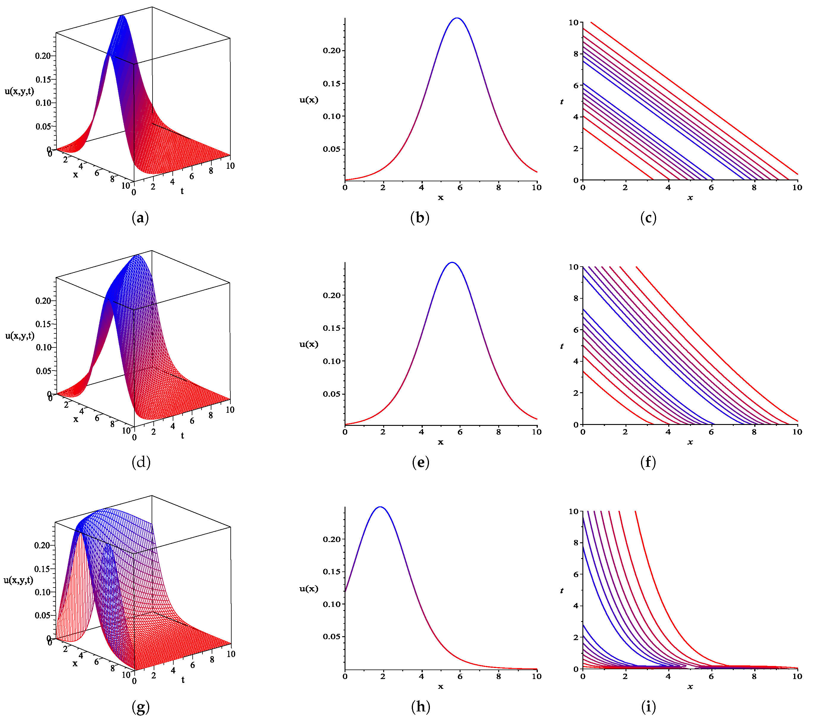
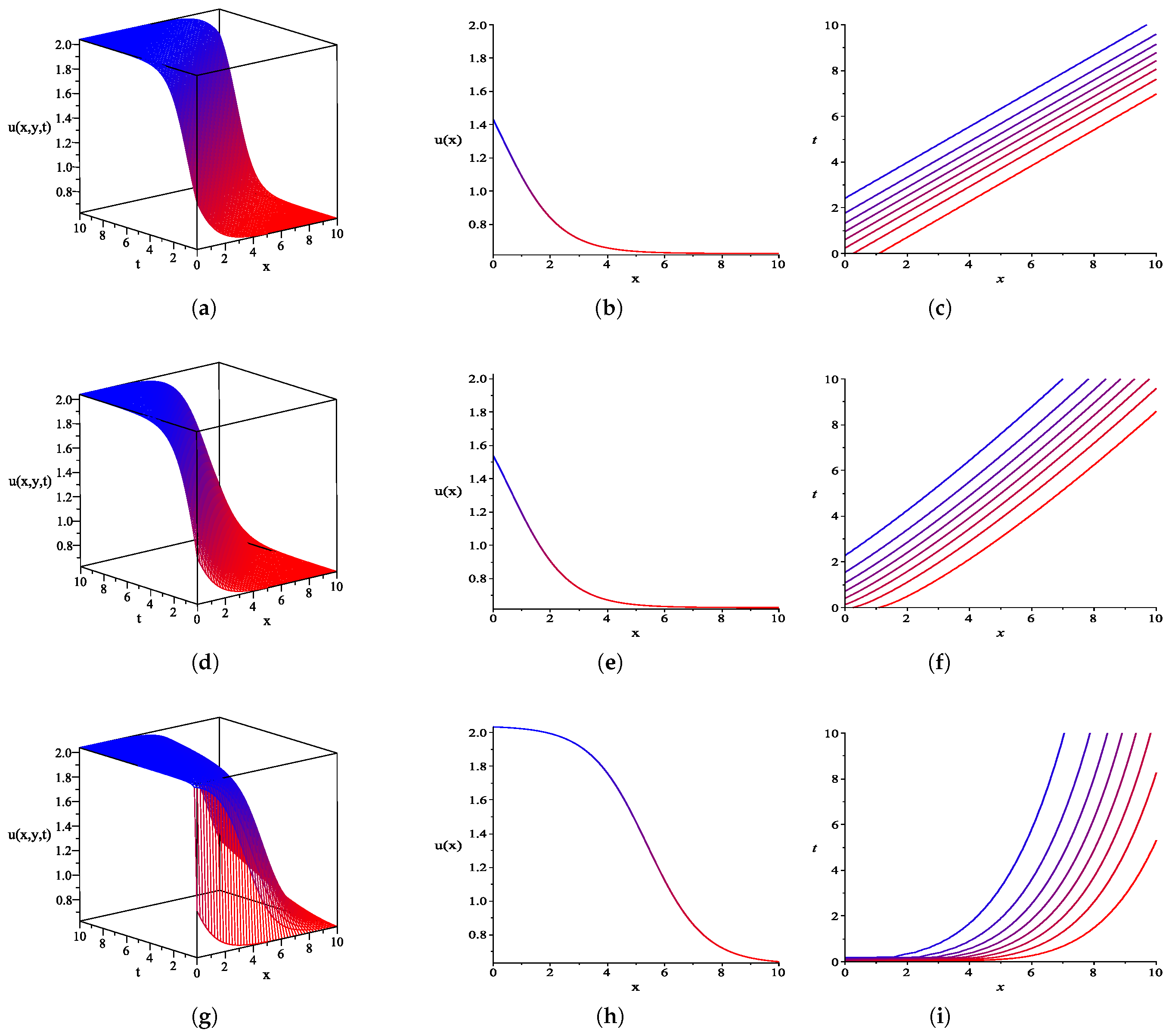
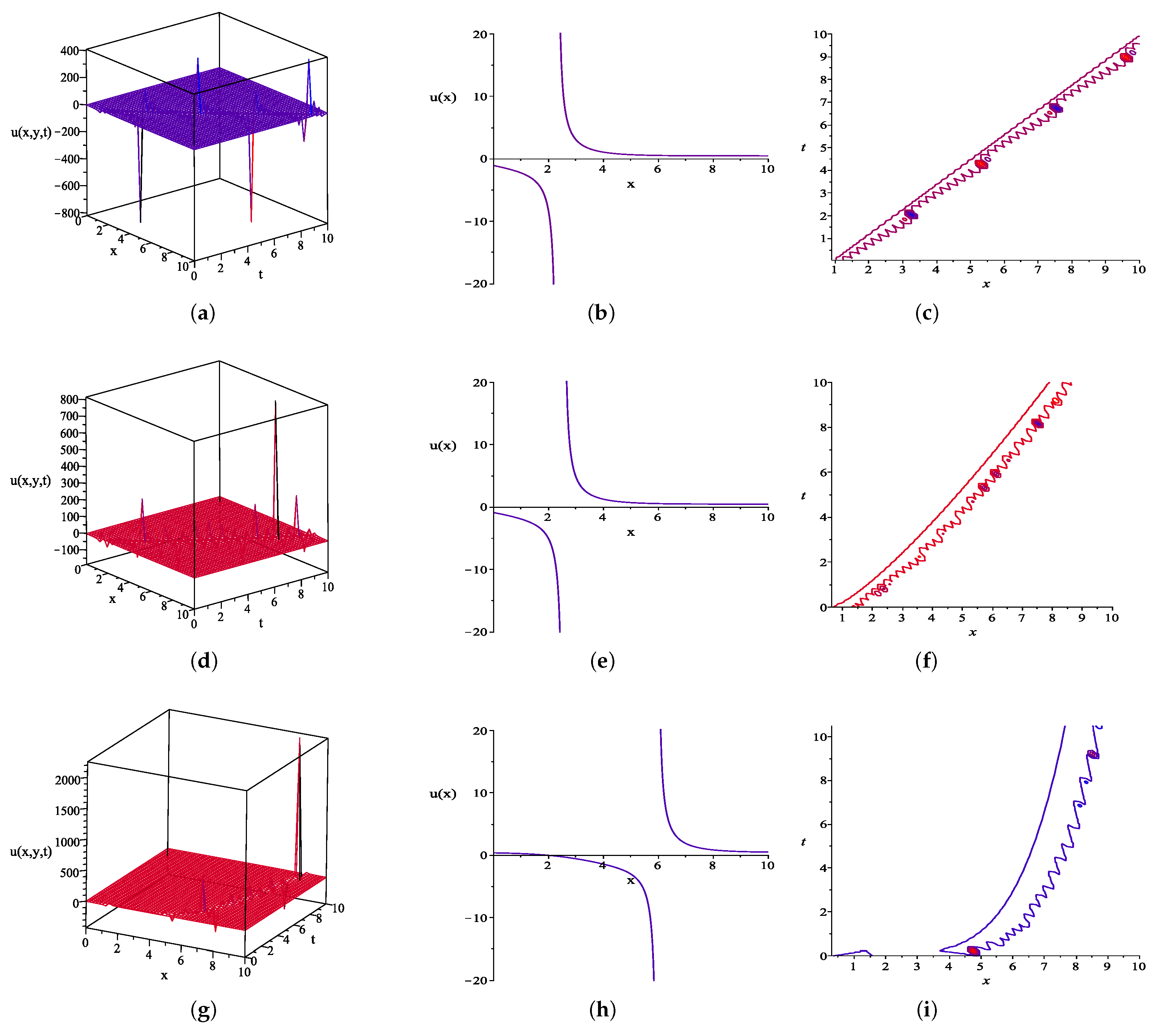
5. Some Graphical Representations

In this section, we provide interesting graphical representations of the exact solutions of the conformable time second integro-differential KP hierarchy Equation (1) obtained using the Exp-function method and of the (2 + 1)-dimensional conformable time partial integro-differential Jaulent–Miodek evolution Equation (2) obtained utilizing the generalized Kudryashov method. The time-fractional order α for the equations is varied in order to explore graphical behaviors of the exact solutions reported in the previous section. In particular, the values of the time-fractional order used for all simulations are α = 1 , 0.8 and 0.2 . The exact solution (30) for Equation (1) and the exact solutions (39) and (43) for Equation (2) are graphically portrayed as 3D, 2D, and contour plots according to the used values of α . All of the 3D plots are drawn on the domain 0 x , t 10 with the fixed value y = 1 . The 2D graphs, showing a relation of u ( x ) and x, are depicted on 0 x 10 with y = t = 1 . Here, the contour plots, presenting a 3D surface by plotting constant u slices on a 2D plane, are plotted to connect the ( x , t ) coordinates, where the given values of u occur and y is fixed at y = 1 . Furthermore, the physical explanations of the displayed graphs are discussed in this section.
In Figure 1, the graphs of the exact solution u ( x , y , t ) in (30), constructed using the Exp-function method, for problem (1) are unfolded in different aspects. Using the values of α as shown above and setting the free parameters a 1 = 1 , b 0 = 5 and b 1 = 0.001 , the solution (30) is evaluated and plotted on the domains for the 3D, 2D, and contour plots in Figure 1. In particular, Figure 1a–c shows the 3D, 2D, and contour plots for solution (30), respectively, when α = 1 . Figure 1d–i are portrayed in the same manner as before except using α = 0.8 and α = 0.2 , respectively. By classifying the shapes of the 3D and 2D graphs in Figure 1, one can identify that solution (30) is a bell-shaped solitary wave solution.
Figure 2 and Figure 3 show the solution graphs for problem (2), which are generated using the generalized Kudryashov method. Specifically, the solution u 1 ( x , y , t ) in (39), in which the top sign of ∓ is chosen, is graphically plotted in Figure 2, and the solution u 2 ( x , y , t ) in (43), in which the top sign of ± is taken, is drawn in Figure 3. Apart from using α = 1 , 0.8 , 0.2 and the domains mentioned above, the following two sets of the parameter values { κ = 1 , p 1 = 3 , p 2 = 3 , p 3 = 3 , p 4 = 5 , p 5 = 1 } and { κ = 1 , p 1 = 3 , p 2 = 1 , p 3 = 1 , p 4 = 0.1 , p 5 = 3 , b 0 = 0.05 , b 1 = 0.6 } are inserted into solution (39) and solution (43), respectively, in order to depict their 3D, 2D, and contour plots. Figure 2a–c demonstrates the 3D, 2D, and contour graphs of the solution u 1 ( x , y , t ) when α = 1 is used. However, the 3D, 2D, and contour plots of the solution u 1 ( x , y , t ) when α = 0.8 and α = 0.2 are shown in Figure 2d–i. The physical behavior of these graphs is characterized as a kink-type solution.
Furthermore, Figure 3a–c displays the 3D, 2D, and contour plots of the solution u 2 ( x , y , t ) in (43) when α = 1 . Proceeding in a similar manner to the above plots, except utilizing α = 0.8 and α = 0.2 , the corresponding graphs are portrayed in Figure 3d–i. As can be seen in the graph structures shown in Figure 3, their physical behavior is considered as a singular multiple-soliton solution.
We can observe some effects of the variation of the time-fractional order α on the 3D and 2D graphs in Figure 1, Figure 2 and Figure 3. It can be possibly concluded that when the value of α is varied to depict the 3D and 2D solutions in each figure, their graphical structures remain the same, but their magnitudes change and translations are detected. In addition, how the magnitude and translation of the 3D and 2D graphs alter depends on the change in α .

6. Discussion and Conclusions

In summary, the Exp-function method, the generalized Kudryashov method, the use of transformation (6), and symbolic software packages such as Maple were successfully employed to obtain exact traveling wave solutions for the conformable time second integro-differential KP hierarchy Equation (1) and the (2 + 1)-dimensional conformable time partial integro-differential JM evolution Equation (2), respectively. Utilizing the Exp-function method to analytically solve Equation (1) and removing the trivial and disqualified solutions, only one exact solution (30) was obtained. As a result, solution (30) is expressed in terms of the exponential functions, or equivalently, the hyperbolic functions, and it behaves as a bell-shaped solitary wave solution under a certain set of parameter values. In order to compare our solution (30) with certain solutions from the relevant literature, one can consider the mathematical expressions between our solution (when α = 1 ) and the solutions in [28,30]. In [28], the generalized Kudryashov method was utilized to solve the second integro-differential KP hierarchy equation for which the exponential function solutions were generated. Their solutions displayed the behavior of a bell-shaped solution. In [30], one of the solutions of the second integro-differential KP hierarchy equation, established by the ( G / G , 1 / G ) -expansion method, was expressed in terms of the hyperbolic functions and characterized as an anti-bell soliton solution. Generally speaking, solution (30) when α = 1 has a mathematical structure similar to that of the solutions in the aforementioned literature.
Applying the generalized Kudryashov method to obtain exact solutions for Equation (2) and after eliminating the trivial solutions, we obtained two different explicit exact solutions, as shown in Equations (39) and (43). The solutions are written in terms of the exponential functions. By plotting these solutions computed using the specific sets of parameter values, a kink-type solution and a singular multiple-soliton solution were obtained. A comparison between our solutions for (2) when α = 1 and the exact solutions of the (2 + 1)-dimensional Jaulent–Miodek equation obtained in [51] is as follows: In [51], the complex method was used to solve the (2 + 1)-dimensional JM equation for which the hyperbolic cotangent function solutions were established. The solutions were characterized as a solitary wave solution of singular kink-type. It can be seen that the structures of their solution and our solution are found in many physical phenomena, such optics and nonlinear waves.
All of the obtained exact solutions discussed in this paper were verified by substituting them back into their corresponding equations with the help of the Maple package program. The Exp-function method and the generalized Kudryashov method are straightforward, reliable, efficient, and pragmatic mathematical tools for solving the proposed equations because they produce uncomplicated exact solution forms. These two methods could be effectively applied to solve a wide range of nonlinear partial integro-differential equations arising in natural phenomena, giving their analytically extracted exact solutions.

Author Contributions

Conceptualization, S.S. (Sekson Sirisubtawee) and S.S. (Surattana Sungnul); methodology, S.K. and S.S. (Sekson Sirisubtawee); software, S.K. and S.S. (Sekson Sirisubtawee); validation, S.K., S.S. (Sekson Sirisubtawee) and S.S. (Surattana Sungnul); formal analysis, S.K. and S.S. (Sekson Sirisubtawee); investigation, S.K. and S.S. (Sekson Sirisubtawee); resources, S.S. (Sekson Sirisubtawee) and S.S. (Surattana Sungnul); data curation, S.K.; writing—original draft preparation, S.K. and S.S. (Sekson Sirisubtawee); writing—review and editing, S.S. (Sekson Sirisubtawee) and S.S. (Surattana Sungnul); visualization, S.K., S.S. (Sekson Sirisubtawee) and S.S. (Surattana Sungnul); supervision, S.S. (Sekson Sirisubtawee) and S.S. (Surattana Sungnul); project administration, S.S. (Sekson Sirisubtawee) and S.S. (Surattana Sungnul); funding acquisition, S.K. and S.S. (Sekson Sirisubtawee). All authors have read and agreed to the published version of the manuscript.

Funding

The first author was funded by King Mongkut’s University of Technology North Bangkok under contract no. KMUTNB-61-PHD-014. The second and third authors were financially supported by the Centre of Excellence in Mathematics, the Commission on Higher Education, Thailand.

Institutional Review Board Statement

Not applicable.

Informed Consent Statement

Not applicable.

Data Availability Statement

Not applicable.

Acknowledgments

The authors are grateful to anonymous referees for the valuable comments which have significantly improved this article. In addition, the first author would like to acknowledge the partial support from the Graduate College, King Mongkut’s University of Technology North Bangkok.

Conflicts of Interest

The authors declare no conflict of interest.

Appendix A

This part demonstrates the expression of each coefficient C i of exp ( i ξ ) , i = 5 , 4 , , 4 , 5 in Equation (25) as follows:
C 5 = k a 1 b 1 4 + 5 a 1 3 b 1 2 2 + 5 a 1 b 1 4 16 + C b 1 5 + 15 a 1 2 b 1 3 4 , C 4 = k a 0 b 1 4 + 35 a 0 a 1 b 1 3 4 + 15 a 0 a 1 2 b 1 2 2 + 10 a 1 2 b 1 2 b 0 + 5 C b 0 b 1 4 + 5 a 1 3 b 0 b 1 + 9 a 1 b 1 3 b 0 16 + a 0 b 1 4 + 4 k a 1 b 0 b 1 3 , C 3 = 10 C b 0 2 b 1 3 + 5 a 1 3 b 1 b 1 + 25 a 1 a 1 b 1 3 2 + k a 1 b 1 4 94 a 1 b 1 b 1 3 4 + 31 a 1 b 1 2 b 0 2 16 + 19 a 0 b 1 3 b 0 16 + 15 a 1 a 1 2 b 1 2 2 + 15 a 0 2 a 1 b 1 2 2 + 25 a 1 2 b 1 b 1 2 4 + 95 a 1 2 b 1 b 0 2 8 + 5 C b 1 b 1 4 + 5 a 1 3 b 0 2 2 + 45 a 0 2 b 1 3 8 + 61 a 1 b 1 4 16 + 4 k a 0 b 0 b 1 3 + 15 a 0 a 1 2 b 0 b 1 + 4 k a 1 b 1 b 1 3 + 6 k a 1 b 0 2 b 1 2 + 20 a 0 a 1 b 0 b 1 2 , C 2 = 19 a 1 b 1 b 0 3 16 + 129 a 1 b 1 3 b 0 16 + 31 a 0 b 1 2 b 0 2 16 + 65 a 1 a 0 b 1 3 4 + 15 a 0 a 1 2 b 0 2 2 + 95 a 0 2 b 1 2 b 0 8 + 10 C b 0 3 b 1 2 + 5 a 1 3 b 1 b 0 6 a 0 b 1 b 1 3 + 55 a 1 a 1 b 0 b 1 2 2 + 4 k a 0 b 1 b 1 3 + 6 k a 0 b 0 2 b 1 2 + 15 a 1 a 0 a 1 b 1 2 + 15 a 1 a 1 2 b 0 b 1 + 15 a 0 2 a 1 b 0 b 1 + 15 a 0 a 1 2 b 1 b 1 + 45 a 1 2 b 1 b 0 b 1 2 + 20 C b 1 b 0 b 1 3 + 4 k a 1 b 0 b 1 3 + 4 k a 1 b 0 3 b 1 + 67 a 1 b 1 2 b 1 b 0 16 + 35 a 0 a 1 b 1 b 1 2 4 + 20 a 0 a 1 b 0 2 b 1 + 12 k a 1 b 1 b 0 b 1 2 + 5 a 0 3 b 1 2 2 + 45 a 1 2 b 0 3 8 , C 1 = 25 2 a 1 a 1 b 1 b 1 2 + 95 a 1 a 1 b 0 2 b 1 4 + 12 k a 0 b 1 b 0 b 1 2 + 12 k a 1 b 1 b 0 2 b 1 + 30 a 0 a 1 b 1 b 0 b 1 + 30 a 1 a 0 a 1 b 0 b 1 + 4 k a 0 b 0 3 b 1 + 15 a 1 a 1 2 b 1 b 1 + 15 a 0 2 a 1 b 1 b 1 + 15 a 0 a 1 2 b 1 b 0 + 30 C b 1 b 0 2 b 1 2 + 4 k a 1 b 1 b 1 3 + 6 k a 1 b 0 2 b 1 2 + 6 k a 1 b 1 2 b 1 2 + 11 a 1 b 1 b 1 b 0 2 8 23 a 0 b 1 b 1 2 b 0 16 + 35 a 1 a 0 b 0 b 1 2 + 15 a 1 2 a 1 b 1 2 2 + 35 a 0 a 1 b 0 3 4 + 151 a 1 b 1 2 b 0 2 16 + 15 a 1 a 0 2 b 1 2 2 + 15 a 0 2 a 1 b 0 2 2 + 15 a 1 a 1 2 b 0 2 2 + 9 a 0 b 1 b 0 3 16 + 55 a 1 2 b 1 2 b 1 4 + 155 a 1 2 b 1 b 0 2 8 + 35 a 0 2 b 1 2 b 1 8 + 10 a 0 2 b 1 b 0 2 + 10 C b 1 2 b 1 3 + 5 C b 0 4 b 1 + 5 a 0 3 b 0 b 1 + k a 1 b 0 4 + 83 a 1 b 1 2 b 1 2 8 29 a 1 b 1 b 1 3 4 + 45 a 1 2 b 1 3 4 + 5 a 1 3 b 1 2 2 + a 1 b 0 4 ,
C 0 = 25 a 0 b 1 b 1 b 0 2 8 + 15 a 1 2 a 0 b 1 2 2 + 15 a 1 a 0 a 1 b 0 2 + 15 a 0 a 1 2 b 1 2 2 + 25 a 1 2 b 1 2 b 0 + 25 a 1 2 b 1 2 b 0 + 30 C b 1 2 b 0 b 1 2 + 20 C b 1 b 0 3 b 1 + 75 a 1 b 0 3 b 1 16 + 10 a 0 b 1 2 b 1 2 + 12 k a 1 b 1 b 0 b 1 2 + 12 k a 1 b 1 2 b 0 b 1 + 6 k a 0 b 1 2 b 1 2 + k a 0 b 0 4 + 35 a 1 a 1 b 0 3 4 + 75 a 1 b 1 b 0 3 16 + 5 a 0 3 b 1 b 1 + C b 0 5 + 15 a 0 2 b 0 3 4 + 5 a 0 3 b 0 2 2 + 5 a 0 b 0 4 16 + 30 a 1 a 1 b 1 b 0 b 1 + 12 k a 0 b 1 b 0 2 b 1 + 15 a 1 2 a 1 b 0 b 1 + 15 a 1 a 0 2 b 0 b 1 + 30 a 1 a 0 a 1 b 1 b 1 + 15 a 1 a 1 2 b 1 b 0 + 15 a 0 2 a 1 b 1 b 0 + 45 a 0 2 b 1 b 0 b 1 4 + 4 k a 1 b 0 3 b 1 + 4 k a 1 b 1 b 0 3 5 a 1 b 1 b 0 b 1 2 16 5 a 1 b 1 b 1 2 b 0 16 + 65 a 1 a 0 b 1 b 1 2 4 + 55 a 1 a 0 b 0 2 b 1 2 + 65 a 0 a 1 b 1 2 b 1 4 + 55 a 0 a 1 b 1 b 0 2 2 , C 1 = 30 C b 1 2 b 0 2 b 1 + 4 k a 1 b 1 3 b 1 + 6 k a 1 b 1 2 b 0 2 + 11 a 1 b 1 b 0 2 b 1 8 23 a 0 b 1 2 b 0 b 1 16 + 35 a 0 a 1 b 1 2 b 0 + 6 k a 1 b 1 2 b 1 2 + 25 a 1 a 1 b 1 2 b 1 2 + 95 a 1 a 1 b 1 b 0 2 4 + 4 k a 0 b 1 b 0 3 + 15 a 1 2 a 0 b 0 b 1 + 15 a 1 2 a 1 b 1 b 1 + 15 a 1 a 0 2 b 1 b 1 + 30 a 1 a 0 b 1 b 0 b 1 + 30 a 1 a 0 a 1 b 1 b 0 + 12 k a 0 b 1 2 b 0 b 1 + 12 k a 1 b 1 b 0 2 b 1 + k a 1 b 0 4 + 83 a 1 b 1 2 b 1 2 8 29 a 1 b 1 3 b 1 4 + 151 a 1 b 1 2 b 0 2 16 + 9 a 0 b 1 b 0 3 16 + 35 a 1 a 0 b 0 3 4 + 15 a 1 2 a 1 b 0 2 2 + 15 a 1 a 0 2 b 0 2 2 + 15 a 1 a 1 2 b 1 2 2 + 15 a 0 2 a 1 b 1 2 2 + 55 a 1 2 b 1 b 1 2 4 + 155 a 1 2 b 1 b 0 2 8 + 35 a 0 2 b 1 2 b 1 8 + 10 a 0 2 b 1 b 0 2 + 5 C b 1 b 0 4 + 10 C b 1 3 b 1 2 + 5 a 0 3 b 1 b 0 + a 1 b 0 4 + 45 a 1 2 b 1 3 4 + 5 a 1 3 b 1 2 2 , C 2 = 55 a 1 a 1 b 1 2 b 0 2 + 12 k a 1 b 1 2 b 0 b 1 + 4 k a 0 b 1 3 b 1 + 6 k a 0 b 1 2 b 0 2 + 15 a 1 2 a 0 b 1 b 1 + 15 a 1 2 a 1 b 1 b 0 + 15 a 1 a 0 2 b 1 b 0 + 15 a 1 a 0 a 1 b 1 2 + 45 a 1 2 b 1 b 0 b 1 2 + 20 C b 1 3 b 0 b 1 + 4 k a 1 b 1 b 0 3 + 4 k a 1 b 1 3 b 0 + 67 a 1 b 1 2 b 0 b 1 16 + 35 a 1 a 0 b 1 2 b 1 4 + 20 a 1 a 0 b 1 b 0 2 + 31 a 0 b 1 2 b 0 2 16 + 15 a 1 2 a 0 b 0 2 2 + 129 a 1 b 1 3 b 0 16 + 65 a 0 a 1 b 1 3 4 + 95 a 0 2 b 1 2 b 0 8 + 10 C b 1 2 b 0 3 + 5 a 1 3 b 0 b 1 + 19 a 1 b 1 b 0 3 16 6 a 0 b 1 3 b 1 + 5 a 0 3 b 1 2 2 + 45 a 1 2 b 0 3 8 , C 3 = k a 1 b 1 4 + 31 a 1 b 1 2 b 0 2 16 9 a 1 b 1 3 b 1 4 + 15 a 1 2 2 a 1 b 1 2 + 15 a 1 a 0 2 b 1 2 2 + 25 a 1 2 b 1 2 b 1 4 + 95 a 1 2 b 1 b 0 2 8 + 5 C b 1 4 b 1 + 10 C b 1 3 b 0 2 + 5 a 1 3 b 1 b 1 + 25 2 a 1 a 1 b 1 3 + 20 a 1 a 0 b 1 2 b 0 + 4 k a 1 b 1 3 b 1 + 6 k a 1 b 1 2 b 0 2 + 4 k a 0 b 1 3 b 0 + 15 a 1 2 a 0 b 1 b 0 + 19 a 0 b 1 3 b 0 16 + 5 a 1 2 3 b 0 2 + 61 a 1 b 1 4 16 + 45 a 0 2 b 1 3 8 , C 4 = 5 C b 1 4 b 0 + 5 a 1 3 b 1 b 0 + 9 a 1 b 1 3 b 0 16 + k a 0 b 1 4 + 35 a 1 a 0 b 1 3 4 + 15 a 1 2 2 a 0 b 1 2 + 10 a 1 2 b 1 2 b 0 + 4 k a 1 b 1 3 b 0 + a 0 b 1 4 , C 5 = 15 a 1 2 b 1 3 4 + 5 a 1 b 1 4 16 + 5 a 1 2 3 b 1 2 + C b 1 5 + k a 1 b 1 4 .

References

  1. Ghafoor, A.; Firdous, S.; Zubair, T.; Iftikhar, A.; Zainab, S.; Mohyud-Din, S.T. (G/G,1/G)-Expansion method for generalized ZK, Sharma-Tasso-Olver (STO) and modified ZK equations. Qscience Connect 2013, 2013, 24. [Google Scholar] [CrossRef]
  2. Aljahdaly, N.H. Some applications of the modified (G/G2)-expansion method in mathematical physics. Results Phys. 2019, 13, 102272. [Google Scholar] [CrossRef]
  3. Zheng, B.; Feng, Q. The Jacobi elliptic equation method for solving fractional partial differential equations. Abstr. Appl. Anal. 2014, 2014, 249071. [Google Scholar] [CrossRef]
  4. Baskonus, H.M.; Sulaiman, T.A.; Bulut, H. Novel complex and hyperbolic forms to the strain wave equation in microstructured solids. Opt. Quantum Electron. 2018, 50, 14. [Google Scholar] [CrossRef]
  5. Eskitasçıoglu, E.; Aktas, M.B.; Baskonus, H.M. New complex and hyperbolic forms for Ablowitz-Kaup-Newell-Segur wave equation with fourth order. Appl. Math. Nonlinear Sci. 2019, 4, 105–112. [Google Scholar] [CrossRef] [Green Version]
  6. Seadawy, A.R. Three-dimensional nonlinear modified Zakharov-Kuznetsov equation of ion-acoustic waves in a magnetized plasma. Comput. Math. Appl. 2016, 71, 201–212. [Google Scholar] [CrossRef]
  7. Seadawy, A.R. Solitary wave solutions of two-dimensional nonlinear Kadomtsev-Petviashvili dynamic equation in dust-acoustic plasmas. Pramana 2017, 89, 49. [Google Scholar] [CrossRef]
  8. Shakeel, M.; Mohyud-Din, S.T.; Iqbal, M.A. Modified extended exp-function method for a system of nonlinear partial differential equations defined by seismic sea waves. Pramana 2018, 91, 1–8. [Google Scholar] [CrossRef]
  9. Yel, G.; Akturk, T. A new approach to (3 + 1)-dimensional Boiti-Leon-Manna-Pempinelli equation. Appl. Math. Nonlinear Sci. 2020, 5, 309–316. [Google Scholar] [CrossRef]
  10. Ryabov, P.N.; Sinelshchikov, D.I.; Kochanov, M.B. Application of the Kudryashov method for finding exact solutions of the high order nonlinear evolution equations. Appl. Math. Comput. 2011, 218, 3965–3972. [Google Scholar] [CrossRef] [Green Version]
  11. Kudryashov, N.A.; Ryabov, P.N.; Fedyanin, T.E.; Kutukov, A.A. Evolution of pattern formation under ion bombardment of substrate. Phys. Lett. A 2013, 377, 753–759. [Google Scholar] [CrossRef]
  12. Sachs, E.; Strauss, A. Efficient solution of a partial integro-differential equation in finance. Appl. Numer. Math. 2008, 58, 1687–1703. [Google Scholar] [CrossRef]
  13. Singh, S.; Patel, V.K.; Singh, V.K. Convergence rate of collocation method based on wavelet for nonlinear weakly singular partial integro-differential equation arising from viscoelasticity. Numer. Methods Partial. Differ. Eqs. 2018, 34, 1781–1798. [Google Scholar] [CrossRef]
  14. Al-Khaled, K.; Darweesh, A.; Yousef, M.H. Convergence of numerical schemes for the solution of partial integro-differential equations used in heat transfer. J. Appl. Math. Comput. 2019, 61, 657–675. [Google Scholar] [CrossRef]
  15. Zadeh, K.S. An integro-partial differential equation for modeling biofluids flow in fractured biomaterials. J. Theor. Biol. 2011, 273, 72–79. [Google Scholar] [CrossRef]
  16. Li, Y.; Liu, X.; Xin, X. Explicit solutions, conservation laws of the extended (2 + 1)-dimensional Jaulent-Miodek equation. arXiv 2015, arXiv:1512.09196. [Google Scholar]
  17. Zheng, X.; Qiu, W.; Chen, H. Three semi-implicit compact finite difference schemes for the nonlinear partial integro-differential equation arising from viscoelasticity. Int. J. Model. Simul. 2020. [Google Scholar] [CrossRef]
  18. Kaewta, S.; Sirisubtawee, S.; Khansai, N. Explicit exact solutions of the (2 + 1)-dimensional integro-differential Jaulent-Miodek evolution equation using the reliable methods. Int. J. Math. Math. Sci. 2020, 2020, 2916395. [Google Scholar] [CrossRef]
  19. Yapman, Ö.; Amiraliyev, G.M.; Amirali, I. Convergence analysis of fitted numerical method for a singularly perturbed nonlinear Volterra integro-differential equation with delay. J. Comput. Appl. Math. 2019, 355, 301–309. [Google Scholar] [CrossRef]
  20. Hendi, F.; Al-Qarni, M. The variational Adomian decomposition method for solving nonlinear two-dimensional Volterra-Fredholm integro-differential equation. J. King Saud Univ. Sci. 2019, 31, 110–113. [Google Scholar] [CrossRef]
  21. Hasseine, A.; Attarakih, M.; Belarbi, R.; Bart, H.J. On the semi-analytical solution of integro-partial differential equations. Energy Procedia 2017, 139, 358–366. [Google Scholar] [CrossRef]
  22. Liu, J.; Zhang, Y.; Wang, Y. Topological soliton solutions for three shallow water waves models. Waves Random Complex Media 2018, 28, 508–515. [Google Scholar] [CrossRef]
  23. Liu, Y.; Wen, X.Y. Soliton, breather, lump and their interaction solutions of the (2 + 1)-dimensional asymmetrical Nizhnik-Novikov-Veselov equation. Adv. Differ. Eqs. 2019, 2019, 332. [Google Scholar] [CrossRef] [Green Version]
  24. Seadawy, A.; Ali, A.; Aljahdaly, N. The nonlinear integro-differential Ito dynamical equation via three modified mathematical methods and its analytical solutions. Open Phys. 2020, 18, 24–32. [Google Scholar] [CrossRef] [Green Version]
  25. Bhrawy, A.; Alhuthali, M.S.; Abdelkawy, M. New solutions for (1 + 1)-dimensional and (2 + 1)-dimensional Ito equations. Math. Probl. Eng. 2012, 1–24. [Google Scholar] [CrossRef] [Green Version]
  26. Lin, L.; Zhu, S.; Xu, Y.; Shi, Y. Exact solutions of Gardner equations through tanh-coth method. Appl. Math. 2016, 7, 2374–2381. [Google Scholar] [CrossRef] [Green Version]
  27. Akbari, M.; Rasht, I. Application of Kudryashov method for the Ito equations. Appl. Math. 2017, 12, 136–142. [Google Scholar]
  28. Gepreel, K.A.; Nofal, T.A.; Alasmari, A.A. Exact solutions for nonlinear integro–partial differential equations using the generalized Kudryashov method. J. Egypt. Math. Soc. 2017, 25, 438–444. [Google Scholar] [CrossRef]
  29. Yin, Y.H.; Ma, W.X.; Liu, J.G.; Lü, X. Diversity of exact solutions to a (3 + 1)-dimensional nonlinear evolution equation and its reduction. Comput. Math. Appl. 2018, 76, 1275–1283. [Google Scholar] [CrossRef]
  30. Miah, M.M.; Ali, H.S.; Akbar, M.A.; Seadawy, A.R. New applications of the two variable (G/G,1/G)-expansion method for closed form traveling wave solutions of integro-differential equations. J. Ocean Eng. Sci. 2019, 4, 132–143. [Google Scholar] [CrossRef]
  31. Alharbi, A.R.; Almatrafi, M.B. New exact and numerical solutions with their stability for Ito integro-differential equation via Riccati–Bernoulli sub-ODE method. J. Taibah Univ. Sci. 2020, 14, 1447–1456. [Google Scholar] [CrossRef]
  32. Khalil, R.; Al Horani, M.; Yousef, A.; Sababheh, M. A new definition of fractional derivative. J. Comput. Appl. Math. 2014, 264, 65–70. [Google Scholar] [CrossRef]
  33. Podlubny, I. Fractional Differential Equations: An Introduction to Fractional Derivatives, Fractional Differential Equations, to Methods of Their Solution and Some of Their Applications; Academic Press: Cambridge, MA, USA, 1999. [Google Scholar]
  34. Yang, S.; Wang, L.; Zhang, S. Conformable derivative: Application to non-Darcian flow in low-permeability porous media. Appl. Math. Lett. 2018, 79, 105–110. [Google Scholar] [CrossRef]
  35. Anderson, D.R.; Camrud, E.; Ulness, D.J. On the nature of the conformable derivative and its applications to physics. arXiv 2018, arXiv:1810.02005. [Google Scholar]
  36. Anderson, D.R.; Ulness, D.J. Newly defined conformable derivatives. Adv. Dyn. Syst. Appl. 2015, 10, 109–137. [Google Scholar]
  37. Chung, W.S. Fractional Newton mechanics with conformable fractional derivative. J. Comput. Appl. Math. 2015, 290, 150–158. [Google Scholar] [CrossRef]
  38. Lazo, M.J.; Torres, D.F. Variational calculus with conformable fractional derivatives. IEEE/CAA J. Autom. Sin. 2016, 4, 340–352. [Google Scholar] [CrossRef]
  39. Çenesiz, Y.; Baleanu, D.; Kurt, A.; Tasbozan, O. New exact solutions of Burgers’ type equations with conformable derivative. Waves Random Complex Media 2017, 27, 103–116. [Google Scholar] [CrossRef]
  40. Birgani, O.T.; Chandok, S.; Dedovic, N.; Radenovic, S. A note on some recent results of the conformable fractional derivative. Adv. Theory Nonlinear Anal. Appl. 2019, 3, 11–17. [Google Scholar]
  41. Gao, F.; Chi, C. Improvement on conformable fractional derivative and its applications in fractional differential equations. J. Funct. Spaces 2020, 2020. [Google Scholar] [CrossRef]
  42. Tasbozan, O.; Çenesiz, Y.; Kurt, A.; Baleanu, D. New analytical solutions for conformable fractional PDEs arising in mathematical physics by exp-function method. Open Phys. 2017, 15, 647–651. [Google Scholar] [CrossRef]
  43. Hosseini, K.; Manafian, J.; Samadani, F.; Foroutan, M.; Mirzazadeh, M.; Zhou, Q. Resonant optical solitons with perturbation terms and fractional temporal evolution using improved tan (ϕ (η)/2)-expansion method and exp function approach. Optik 2018, 158, 933–939. [Google Scholar] [CrossRef]
  44. Yaslan, H.Ç.; Girgin, A. Exp-function method for the conformable space-time fractional STO, ZKBBM and coupled Boussinesq equations. Arab. J. Basic Appl. Sci. 2019, 26, 163–170. [Google Scholar] [CrossRef] [Green Version]
  45. Ghany, H.A.; Hyder, A.A.; Zakarya, M. Exact solutions of stochastic fractional Korteweg de-Vries equation with conformable derivatives. Chin. Phys. B 2020, 29, 030203. [Google Scholar] [CrossRef]
  46. Biswas, A.; Sonmezoglu, A.; Ekici, M.; Mirzazadeh, M.; Zhou, Q.; Moshokoa, S.P.; Belic, M. Optical soliton perturbation with fractional temporal evolution by generalized Kudryashov’s method. Optik 2018, 164, 303–310. [Google Scholar] [CrossRef]
  47. El-Ganaini, S.; Al-Amr, M.O. New abundant wave solutions of the conformable space-time fractional (4 + 1)-dimensional Fokas equation in water waves. Comput. Math. Appl. 2019, 78, 2094–2106. [Google Scholar] [CrossRef]
  48. Wazwaz, A.M. Kadomtsev-Petviashvili hierarchy: N-soliton solutions and distinct dispersion relations. Appl. Math. Lett. 2016, 52, 74–79. [Google Scholar] [CrossRef]
  49. Gepreel, K.A. Exact solutions for nonlinear integral member of Kadomtsev-Petviashvili hierarchy differential equations using the modified (w/g)-expansion method. Comput. Math. Appl. 2016, 72, 2072–2083. [Google Scholar] [CrossRef]
  50. Zhang, Y.Y.; Liu, X.Q.; Wang, G.W. Symmetry reductions and exact solutions of the (2 + 1)-dimensional Jaulent-Miodek equation. Appl. Math. Comput. 2012, 219, 911–916. [Google Scholar] [CrossRef]
  51. Gu, Y.; Deng, B.; Lin, J. Exact traveling wave solutions to the (2 + 1)-dimensional Jaulent-Miodek equation. Adv. Math. Phys. 2018, 2018. [Google Scholar] [CrossRef]
  52. Ma, H.C.; Deng, A.P.; Yu, Y.D. Lie symmetry group of (2 + 1)-dimensional Jaulent-Miodek equation. Therm. Sci. 2014, 18, 1547–1552. [Google Scholar] [CrossRef]
  53. Matinfar, M.; Eslami, M.; Roshandel, S. The first integral method to study the (2 + 1)-dimensional Jaulent-Miodek equations. Pramana 2015, 85, 593–603. [Google Scholar] [CrossRef]
  54. Kaplan, M.; Bekir, A.; Akbulut, A. A generalized Kudryashov method to some nonlinear evolution equations in mathematical physics. Nonlinear Dyn. 2016, 85, 2843–2850. [Google Scholar] [CrossRef]
  55. Sirisubtawee, S.; Koonprasert, S.; Sungnul, S. Some Applications of the (G/G,1/G)-expansion method for finding exact traveling wave solutions of nonlinear fractional evolution equations. Symmetry 2019, 11, 952. [Google Scholar] [CrossRef] [Green Version]
  56. Sirisubtawee, S.; Koonprasert, S.; Sungnul, S.; Leekparn, T. Exact traveling wave solutions of the space-time fractional complex Ginzburg-Landau equation and the space-time fractional Phi-4 equation using reliable methods. Adv. Differ. Eqs. 2019, 2019, 219. [Google Scholar] [CrossRef]
  57. Sirisubtawee, S.; Koonprasert, S.; Sungnul, S. New exact solutions of the conformable space-time Sharma-Tasso-Olver equation using two reliable methods. Symmetry 2020, 12, 644. [Google Scholar] [CrossRef] [Green Version]
  58. Al-Ghafri, K.S. Soliton behaviours for the conformable space-time fractional complex Ginzburg-Landau equation in optical fibers. Symmetry 2020, 12, 219. [Google Scholar] [CrossRef] [Green Version]
  59. He, J.H.; Elagan, S.; Li, Z. Geometrical explanation of the fractional complex transform and derivative chain rule for fractional calculus. Phys. Lett. A 2012, 376, 257–259. [Google Scholar] [CrossRef]
  60. Su, W.H.; Yang, X.J.; Jafari, H.; Baleanu, D. Fractional complex transform method for wave equations on Cantor sets within local fractional differential operator. Adv. Differ. Eqs. 2013, 2013, 97. [Google Scholar] [CrossRef] [Green Version]
  61. Güner, O.; Bekir, A.; Cevikel, A.C. A variety of exact solutions for the time fractional Cahn-Allen equation. Eur. Phys. J. Plus 2015, 130, 146. [Google Scholar] [CrossRef]
  62. Rahmatullah; Mohyud-Din, S.T.; Khan, U. Exact traveling wave solutions of fractional order Boussinesq-like equations by applying Exp-function method. Results Phys. 2018, 8, 114–120. [Google Scholar] [CrossRef]
  63. Guner, O.; Aksoy, E.; Bekir, A.; Cevikel, A.C. Different methods for (3 + 1)-dimensional space-time fractional modified KdV-Zakharov-Kuznetsov equation. Comput. Math. Appl. 2016, 71, 1259–1269. [Google Scholar] [CrossRef]
  64. Guner, O.; Bekir, A. The Exp-function method for solving nonlinear space-time fractional differential equations in mathematical physics. J. Assoc. Arab. Univ. Basic Appl. Sci. 2017, 24, 277–282. [Google Scholar] [CrossRef] [Green Version]
  65. Demiray, S.T.; Bulut, H. Soliton solutions of some nonlinear evolution problems by GKM. Neural Comput. Appl. 2019, 31, 287–294. [Google Scholar] [CrossRef]
  66. He, J.H.; Wu, X.H. Exp-function method for nonlinear wave equations. Chaos Solitons Fractals 2006, 30, 700–708. [Google Scholar] [CrossRef]
Figure 1. Associated plots of u ( x , y , t ) in Equation (30) obtained using the Exp-function method: (ac) 3D plot, 2D plot, and contour plot when α = 1 ; (df) 3D plot, 2D plot, and contour plot when α = 0.8 ; (gi) 3D plot, 2D plot, and contour plot when α = 0.2 .
Computation 09 00052 g001
Figure 2. Associated plots of u 1 ( x , y , t ) in Equation (39) obtained using the generalized Kudryashov method: (ac) 3D plot, 2D plot, and contour plot when α = 1 ; (df) 3D plot, 2D plot, and contour plot when α = 0.8 ; (gi) 3D plot, 2D plot, and contour plot when α = 0.2 .
Computation 09 00052 g002
Figure 3. Associated plots of u 2 ( x , y , t ) in Equation (43) obtained using the generalized Kudryashov method: (ac) 3D plot, 2D plot, and contour plot when α = 1 ; (df) 3D plot, 2D plot, and contour plot when α = 0.8 ; (gi) 3D plot, 2D plot, and contour plot when α = 0.2 .
Computation 09 00052 g003
Publisher’s Note: MDPI stays neutral with regard to jurisdictional claims in published maps and institutional affiliations.

